


Introduction
According to the National Snow and Ice Data Center (NSIDC, 2006), sea ice is defined as frozen ocean surface water that forms, grows and melts into the sea and primarily occurs in both the Arctic and Antarctic oceans. In the Northern Hemisphere (NH), the occurrence of sea ice has been reported down to a southern limit of 38°N near Bohai Bay, China, while in the Southern Hemisphere (SH), sea ice develops around the Antarctic continent, with a northern limit of ~55°S (NSIDC, 2006). Generally, sea ice forms and grows during winter and melts during summer, with some sea ice only lasting one season and some persisting for multiple seasons.
In complex environments such as fjords, the interaction between ocean and fresh water from multiple sources (e.g. surface and ground runoff, rivers, snow/glacier melt and precipitation) produces strong vertical and horizontal gradients in salinity, density and organic and inorganic material, the last of which is an important source of nutrients (Pickard, Reference Pickard1971; Iriarte and others, Reference Iriarte, Pantoja and Daneri2014). Oceanographically, the fjords and channels of southern Chile may be considered as a transitional marine system influenced by deep oceanic waters with high salinity that are rich in nutrients and fresh surface water with low salinity that is low in nutrients (Schneider and others, Reference Schneider2014). The relationship among sea-ice conditions, iceberg plume production and air temperature was assessed in a study conducted in Canada (Herdes and others, Reference Herdes, Copland, Danielson and Sharp2012), which indicated that large volumes of ice detached from the fronts of the tidewater glaciers when the air temperature was above 0°C and that sea ice formed under conditions of low nighttime air temperature.
The presence and extent of sea ice in polar regions have been extensively studied due to its implications for Arctic, Antarctic, fjord and marine ecosystems (Stammerjohn and others, Reference Stammerjohn, Martinson, Smith and Iannuzzi2008; Ainley and others, Reference Ainley, Tynan and Stirling2010; Massom and Stammerjohn, Reference Massom and Stammerjohn2010; Acevedo and others, Reference Acevedo, González, Garthe, González, Gómez and Aguayo-Lobo2017), its role as an integral component of the climate system (Simmonds and Budd, Reference Simmonds and Budd1991; Yuan and Martinson, Reference Yuan and Martinson2000; Raphael, Reference Raphael2003; Barreira, Reference Barreira2008; Meier and others, Reference Meier2014; Goosse, Reference Goosse2015) and its ability to show an early response to climate change (Eicken and Lemke, Reference Eicken and Lemke2001). With the snow and sea-ice surface being highly reflective of solar radiation (compared with an ice-free water surface), the presence of sea ice is crucial for the surface energy balance (Gerland and Renner, Reference Gerland and Renner2007).
Floating ice found in the Cordillera Darwin (CD) fjords had previously been thought to be land ice calved from the many CD tidewater glaciers. In this study, with a key contribution from a citizen observation from a commercial airplane of a peculiar ice floe on the inland waters of CD, we have found a land-fast sea-ice formation over the CD fjords. The purpose of this paper is to describe the first observations of sea ice above the previously identified northern limit in the Southern Hemisphere and to highlight new areas of sea-ice formation in regions previously not considered propitious to identify the climatic and oceanographic conditions associated with this phenomenon.
Study area
The CD is a mountain range (Fig. 1) located at the southernmost tip of the Andes, with its icefield covering an area of 2600 km2, extending ~200 km west-east from 71.8° W to 68.5° W and ~50 km south-north from 54.9° S to 54.2° S. The ice field is bordered to the north by the Almirantazgo fjord and to the south by the Beagle Channel. Mean daily temperature patterns indicate a regional control, with temperatures varying between 0 and 15°C at sea level (Fernandez and others, Reference Fernandez, Anderson, Wellner and Hallet2011), with little variation between summer and winter, especially near the coast, where the temperature becomes more maritime influenced (Holmlund and Fuenzalida, Reference Holmlund and Fuenzalida1995).

Fig. 1. Study area in southern South America with the Cordillera Darwin Ice Field (CDI) highlighted, the Darwin Mountain (red point) and the delimitation of water surface into the fjords (black lines). Fjords analyzed: Cuevas (1), Parry (2), Marinelli (3), Finland (4), Auer (5), Relander (6), Hyatt (7), Serrano (8), Ventisquero (9), Garibaldi (10), Torcido (11), Pia West (12) and Pia East (13). The scale that applies to the center point of the map.
The CD is characterized by high annual precipitation, averaging ~5000–10 000 mm (Garreaud and others, Reference Garreaud, Lopez, Minvielle and Rojas2013). During winter, rainfall in the region comes predominantly from the south and southwest (Holmlund and Fuenzalida, Reference Holmlund and Fuenzalida1995). The E–W orientation of the mountain ridge generates an orographic effect with higher snowfall in its southern and western portions, whereas warmer and drier conditions are identified in the glaciers located in the northern and eastern parts of the CD (Holmlund and Fuenzalida, Reference Holmlund and Fuenzalida1995). In general, glaciers of the CD are classified as temperate maritime glaciers because of their mid-latitude position and climatic conditions (Rosenblüth and others, Reference Rosenblüth, Fuenzalida and Aceituno1995).
The Chilean fjords extend from 42° to 55° S and include more than 3000 islands, and this intricate geographical maze remains isolated and poorly understood. The best information that is available today comes from different research cruises carried out more than 10 years ago, with sparse measurements taken due to the vastness of the area. Water masses, salinity gradients, bathymetry, biochemistry and other parameters were studied during these different cruises (Sievers, Reference Sievers1994; Silva and others, Reference Silva, Sievers and Prado1995; Sievers and others, Reference Sievers, Calvete and Silva2002; Silva and others, Reference Silva, Guzmán and Valdenegro2003; Valdenegro and Silva, Reference Valdenegro and Silva2003; Sievers, Reference Sievers2008).
Fjord hydrology is usually characterized by a vertical two-layered structure with a highly variable 5- to 10-m-thick freshwater surface layer and a more uniform, saltier lower layer (Sievers and others, Reference Sievers, Calvete and Silva2002; Dávila and others, Reference Dávila, Figueroa and Müller2002), while studies carried out in the surroundings of the CD indicate that the depth of the upper layer can vary according to the latitude of the fjords. In the CD region, depth limits are between 50 and 75 m, and a more homogeneous layer lies below this depth. This layer is not influenced by factors such as solar radiation; the addition of heated or cooled water by rivers, glaciers or precipitation; or vertical mixing caused by wind (Sievers and others, Reference Sievers, Calvete and Silva2002). However, colder surface water with weak stratification, along with little difference in salinity between the surface and lower layer, is observed during winter (Salcedo-Castro and others, Reference Salcedo-Castro, Montiel, Jara and Vásquez2014). In addition, the tidal glaciers present in the CD contribute most of the fresh water by discharging subglacial and englacial flows. This volume of fresh water within the fjords can contribute to the reduction in the salinity of surface water to the point of favoring the onset of sea-ice formation.
Recent studies of the CD demonstrate that this region has experienced a rapid reduction in the area covered by glaciers (Rivera and Casassa, Reference Rivera and Casassa2004; Masiokas and others, Reference Masiokas2009; Lopez and others, Reference Lopez2010; Willis and others, Reference Willis, Melkonian, Pritchard and Rivera2012; Melkonian and others, Reference Melkonian2013; Meier and others, Reference Meier2019). The most substantial retreat was that of the Marinelli Glacier, which detached from a prominent terminal moraine after 1960, with a retreat rate of 787 m a−1 between 1992 and 2000 (Porter and Santana, Reference Porter and Santana2003). According to Melkonian and others (Reference Melkonian2013), from 2001 to 2003, the glaciers located in the CD presented flow velocities in the terminal portions of ~10 m d−1. Furthermore, these authors estimated glacier losses of up to 20 m in height each year in the region during the period from 2001 to 2011.
In particular, the shallow depth of the eastern end of the Beagle Channel restrains the influx of subsurface ocean waters (Antezana, Reference Antezana1999). As water exchange with the Pacific is limited and occurs through narrow and shallow openings, most of the water that fills the Magellan and Fuegian basins must be semi-isolated. These bathymetric features and lateral contractions within the inner passages, which affect water circulation, also help to explain the hydrographic characteristics and subdivisions of micro-catchments around the CD (Antezana, Reference Antezana1999).
In temperate fjords, the stratification alternates according to the time of year, varying between two layers of circulation during spring (discharge of melted snow) and summer (discharge of melting ice) and vertically homogeneous estuarine conditions during winter (Syvitski and Skei, Reference Syvitski and Skei1983). The freshwater plume flowing within a fjord is commonly divided into two zones (Syvitski, Reference Syvitski1986): a near zone (upper prodelta), in which the energy of the river discharge controls the spreading and mixing of the surface plume with its surroundings, and a far region (lower prodelta), in which external agents control the transport and mixing.
Valdenegro and Silva (Reference Valdenegro and Silva2003) presented in situ observations of temperature and salinity collected in spring 1998 that showed a relatively stable surface layer of ~5.5°C in the southernmost part of Almirantazgo Fjord. In the surface layer, the salinity ranged from 28 to 30.5 psu, and below this layer, at the head of Almirantazgo Fjord, the highest gradients were measured on the order of 3 psu per 10 m, corresponding to a very strong halocline, whereas below depths of 200 m, the water column presented homogeneous values of ~31 psu.
Materials and methods
In the current study, 13 fjords were selected along the CD (Fig. 1), all of which were associated with one or more tidewater glaciers. Satellite images permitted visual identification of the sea-ice layer, generating adequate spatial and temporal data. Once the targets identified were classified as sea ice, polygons were generated manually to delimit the surface area of the occurrences. Meteorological data described the atmospheric forcing during 2015, whereas data from previous years were obtained from a climatological model (NCEP/NCAR Reanalysis 1 model), with the aim of generating a comparison between the spatial and temporal results obtained from satellite images. In addition, photographs taken from a commercial airplane flying over the CD region, traveling from Puerto Williams to Punta Arenas (Fig. 3b), and the photographs acquired with the support of a Chilean Navy helicopter within the Cuevas and Parry fjords were examined.
Satellite data
To describe the occurrence of sea ice in the CD fjords, we selected a time series of Landsat 4–5 Thematic Mapper (TM), Landsat-7 Enhanced TM (ETM) and Landsat-8 Operational Land Imager (OLI) optical band images acquired between June and October from 2000 to 2017. For a more in-depth analysis of 2015, we combined information from images acquired by the satellite sensors Sentinel-1 synthetic aperture radar (SAR) and Landsat-8 OLI images (Fig. 2). Sentinel-1, launched in April 2014, is one of the new-generation SAR satellites from the European Space Agency (ESA). This program ensures the continuity of SAR C-band data acquisition (Berger and others, Reference Berger, Moreno, Johannessen, Levelt and Hanssen2012), with open and free access to data for all users. For this research, images were selected in ground range detected (GRD) and interferometric wide swath (IW) acquisition modes (Berger and others, Reference Berger, Moreno, Johannessen, Levelt and Hanssen2012). In both acquisition modes, images covered 250 km × 250 km of the ground, with a 10-m spatial resolution, incidence angles between 29.1° and 46° (Berger and others, Reference Berger, Moreno, Johannessen, Levelt and Hanssen2012), and vertical–vertical (VV) polarization. Launched in 2013, Landsat-8 is the latest version of the Landsat satellite series and requires cloud-free and daylight conditions for observations. Its OLI has a spatial resolution of 30 m, covering 185 km × 180 km (Fig. 2).

Fig. 2. Sentinel-1 and Landsat-8 footprints of images acquired during 2015. Indicated by stars are the locations of meteorological stations at Condor River, Azopardo River and Navarino Port. The tide gauge from the Chilean General Water Board (DGA) at Dawson Island is indicated by a point. The scale bar applies to the center point of the map.
The signature of the surface at the SAR bands is sensitive to roughness and moisture content such that smooth or moist surfaces usually appear dark while rough or dry surfaces often appear bright (Herdes and others, Reference Herdes, Copland, Danielson and Sharp2012). The energy reflected by a target, or backscattering, depends mostly on the frequency and wavelength of the emitted pulse, the properties of the surface (e.g. slope, roughness and density) and how the pulse is reflected, scattered, absorbed and/or transmitted by the object (Pellikka and Rees, Reference Pellikka and Rees2010). In this study targets identified as ice, whether sea ice or small drifting growlers, have higher backscatter than water. Due to this contrast, the brightest objects can be defined as ice, while the darker targets are identified as ice-free water surfaces. Also, comparison with optical imagery was used as a way of validation. For growlers and sea-ice identification in Sentinel-1, Landsat 4-5 TM, Landsat-7 ETM and Landsat-8 OLI images, sea ice was considered to have a smooth and homogeneous texture: in contrast, growlers form a rough texture on the ocean surface in the same way that land-fast sea-ice fracture patterns and sea-ice drift patterns of growlers aid in the classification of the targets in the satellite images.
In total, 54 satellite images were selected from 2000 to 2017 (Tables 1–3), and 28 satellite images were selected from 2015 (Fig. 5). The sea-ice area in each image was manually defined and used to calculate sea-ice area. When sea ice was identified within the same fjord in two or more satellite images for the same year, the image with the largest sea-ice extent was used for area calculations (Tables 2 and 3).
Table 1. Satellite images used in the identification of sea ice within the fjords of the Darwin Mountain Range between June and October for the period from 2000 to 2017, grouped per 30 days when possible

The • signals that sea ice was identified the respective fjord that day. Fjords analyzed: Cuevas (1), Parry (2), Marinelli (3), Finland (4), Auer (5), Relander (6), Hyatt (7), Serrano (8), Ventisquero (9), Garibaldi (10), Torcido (11), Pia West (12) and Pia East (13), as shown in Figure 1.
Table 2. Recorded occurrence of sea ice in the CD fjords from June to October for the period 2000 to 2017

In order of importance: reason between the number of times that sea ice was detected/number of times that fjord was observed. The last two lines indicate the sum of all sea-ice areas in each year and the proportion of the total area of all the CD fjords. The last column on the right shows the percentage of sea-ice occurrence for each of the 13 fjords analyzed.
Table 3. Area measurement of sea ice for each fjord when sea ice was identified and the corresponding proportion compared with the total area of the fjord

The last two lines indicate the sum of all sea-ice area in each year and the proportion of the total area of all the CD fjords. The years 2010 and 2011 are not included in the table since there were no data recorded.
Meteorological data
In situ observational records of temperature and precipitation for the year 2015 were obtained from the Explorador Climatico CR2 (http://explorador.cr2.cl/), a site that contains meteorological information from the Meteorological Office of Chile (www.meteochile.gob.cl), and the General Directorate of Waters (www.dga.cl). These data were collected by three automatic meteorological stations selected due to their proximity to the Cuevas fjord (Fig. 2): Condor River (53.99° S, 70.06° W, 0 m, 93 km distance), Azopardo River (54.50° S, 68.83° W, 32 m a.s.l., 40 km distance) and Navarino Port (54.92° S, 68.32° W, 0 m a.s.l., 69 km distance). These stations obtain hourly data values for air temperature and daily accumulated precipitation.
The closest weather station to the Cuevas fjord, located in Azopardo River, did not collect data on 47 consecutive days from 25 June to 10 October 2015. To fill this gap, correlations were made with data from other close stations (i.e. Condor River and Navarino Port), and missing data from the weather station nearest to Cuevas fjord were replaced by data from the Condor River station due to the high correlation between these two stations (R 2: 0.8384 and RMSE: 1.485). Missing data from the weather station closest to the Cuevas fjord was replaced by data from the Condor River station due to the high correlation between these two stations (R 2: 0.5148; RMSE: 2.335).
To estimate the influence of meteorological conditions during the period of sea-ice formation, atmospheric information from the NCEP/NCAR Reanalysis 1 model was used (Kistler and others, Reference Kistler2001). This dataset consists of a reanalysis of atmospheric data from 1948 to the present. Its standard resolution is 2.5°, with a temporal resolution of 6 h. For the current analysis, we used monthly air temperature data from 1980 to 2017. In the global grid of the model, the nearest point to the CD, 55°S and 70°W, was selected.
Results and discussion
Sea-ice observation in the Cuevas fjord and meteorological conditions in 2015
On 29 September 2015, a passenger in an airplane flying over the CD region noticed a large ice floe in the Almirantazgo fjord and provided photographs for the researchers at CEQUA (Fig. 3b). In one Landsat-8 OLI image obtained ~1 week prior to the airplane sighting, the same ice floe was visible in the Cuevas fjord (Fig. 3a) at a position ~30 km from the location of the sighting on 29 September 2015.

Fig. 3. Satellite Landsat-8 image on 22 September 2015 identifying the occurrence of sea ice in Cuevas fjord (a). The same floe was captured later by oblique aerial photography on 29 September 2015 by an aircraft passenger (b). The scale bar applies to the center point of the map.
On 6 October 2015, a helicopter flew over Cuevas and Parry fjords, identifying once again the occurrence of ice floes over a large part of the water surface area of both fjords (Fig. 4). Because of the remote area and the lack of landing space, direct measurements of sea-ice freeboard were impossible to make, and the helicopter images taken were not sufficient for a reliable estimation. Using a sequence of images from Landsat-8, the fragmentation of the land-fast sea-ice formation associated with the sea-ice floe sighted on 29 September 2015 could be observed (Fig. 3).

Fig. 4. Photographs taken on 6 October 2015 with the support of a helicopter from the Chilean Navy, identifying the presence of large floes of sea ice inside two fjords: Parry (a) and Cuevas (b).
Additionally, by evaluating 28 SAR satellite images from 2015, we identified the presence of drifting glacial ice (i.e. growlers) and land-fast sea ice in the Cuevas fjord, which was mainly concentrated in the southern region of the fjord, closest to the glacier, where growlers are produced by calving (Fig. 6). Additionally, the sea-ice formation seemed to be land-fasted in origin and next to the head of the glacier. It should be noted that the occurrence of sea ice inside Cuevas fjord was restricted to only the winter and early springtime period, which can be observed in satellite images 15–20 (Fig. 5).

Fig. 5. (a) Cropped Sentinel-1 satellite images acquired during 2015 showing variability in ice occurrence in Cuevas fjord (images have been stretched for visualization purposes). (b) Proportions ($\%$ ) of area covered by sea ice (white pixels identified on satellite numbers 15–20), icebergs (white pixels identified on satellite numbers 1–14 and 21–28) and ice-free water (pixels in black) within the fjord.
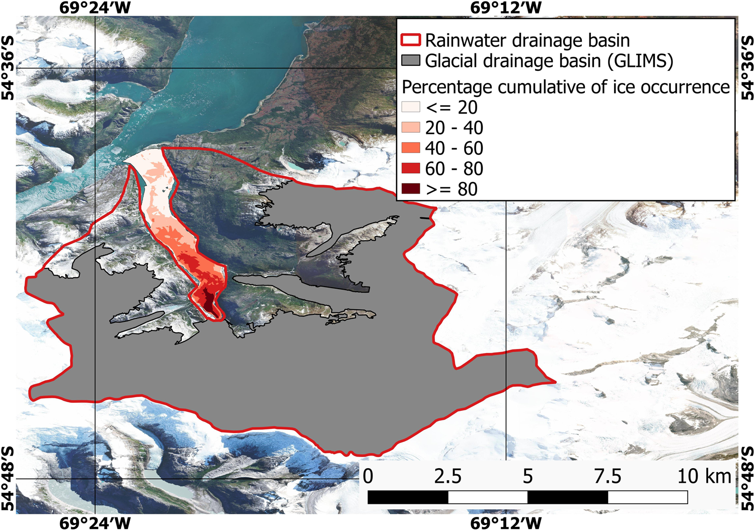
Fig. 6. Cumulative percentage of ice occurrence in 2015 inside Cuevas fjord, where the highest occurrence of ice is associated with the proximity of the tidal water glacier. The area and boundary of the drainage basin are marked in gray and red, respectively.
According to the backscatter pattern of the SAR sensor, we could identify the pixels in white as floating ice and the pixels in black as water. Based on this contrast, we can infer that growlers were predominant during the first and last months of 2015 (i.e. January to May and October to December). This period experienced a high occurrence of growlers from tidewater glaciers, whereas in the winter and early springtime months (i.e. July to September), we identified a pattern of sea ice (white pixels) abundance within Cuevas fjord (Fig. 5a, satellite images 17, 18 and 20). Images 14 and 15 show the maximum area of ice on the fjord, but the pixel backscatter observed can be better interpreted as a mix of growlers and sea ice that is not yet consolidated.
The 2015 atmospheric temperature data analyzed from the nearby AWS stations showed that the occurrence of sea ice in the Cuevas fjord corresponded to a period of low air temperatures (Fig. 7). The daily mean air temperatures between the beginning of June and the end of September were below 0°C for ~74$\%$ of the period, with a mean air temperature for the four combined months of − 1.18°C. Based on different observed surface salinities of 28–30.5 (Valdenegro and Silva, Reference Valdenegro and Silva2003) the expected freezing ocean temperature for the area should be − 1.8°C. There were 58 days, or $48\%$
 of the period, with a mean air temperature below the expected freezing point.

Fig. 7. (a) Surface air temperature during 2015 at the Azopardo River station: recorded daily minimum (blue) and maximum (red) values of surface air temperature, and (b) cumulative measures of daily precipitation at the Azopardo River station. Numbers on the top and dotted lines show the 2015 acquisition dates of Sentinel-1 and Landsat-8 satellite images used in this study.
Between satellite acquisitions 18 and 19, the air temperature remained below zero degrees for 7 consecutive days, and the mean air temperature remained below zero degrees for 8 consecutive days. Between acquisitions 20 and 21, the air temperature was below zero degrees for 6 consecutive days, and the mean air temperature remained below zero degrees for 10 consecutive days. These extended cold periods are probably the reason that sea ice in the Cuevas fjord remained present for almost the entire winter period, even after a reduction in ice coverage over the fjord, as noted between acquisitions 15 and 16. This effect could be attributed to the consolidation of sea ice, with growlers occupying a larger area. Drifting ice from calving could become trapped in the sea ice from that point on or exit the fjord. The positive mean air temperatures measured after satellite acquisition 21 were likely responsible for the fragmentation that generated the sea ice identified in the photograph taken on 29 September 2015.
Snow on sea ice is a complex medium that is strongly coupled to atmospheric, oceanic and sea-ice conditions and is thus heterogeneous across space and time (Webster and others, Reference Webster2018). Evaluating the measured precipitation values at the Azopardo River weather station (Fig. 7), the period between July and September is the interval with the highest amount of accumulated precipitation (~396 mm). This volume of precipitation, concentrated in this period, may have had the capacity to decrease the surface water salinity within the fjords locally. Additionally, the highest amount of precipitation occurred during the lowest temperature periods in winter, and solid precipitation (i.e. snow) occurred above sea ice, as can be seen in the field photographs (Fig. 4).
Daily temperature data from 2015 allowed for the visualization of specific conditions under which sea-ice formation occurred, while average monthly data reveal temperature anomalies in the study area. In this manner, the reanalyzed NCEP/NCAR Reanalysis 1 (Kistler and others, Reference Kistler2001) data provide a good overview of what occurred during the presence of sea ice and, at the same time, allow the visualization of a historical panorama of atmospheric patterns and conditions in the CD region over the past few decades (Fig. 8).

Fig. 8. Air surface temperature anomaly (NCEP/NCAR Reanalysis 1) values between 1980 and 2017. A negative temperature anomaly is observed for almost the entire year of 2015.
Analysis of the monthly temperature anomaly time series showed that November 2009 ( − 2.95) had the most negative value of the record, that 1980, 1986, 1991 and 2015 had more than 9 months of negative temperature anomalies, and that the years with the most negative cumulative temperature anomalies (without considering the positive months) were 1986 ( − 9.99), 2012 ( − 9.97) and 2015 ( − 9.84). These data support the interpretation that prolonged periods of low temperatures are the main reason for the generation and duration of sea ice on the Patagonian fjords. Nevertheless, data from Landsat imagery presented in the next sections (Table 2) do not appear to support this interpretation, but this discrepancy could be due to the lack of good optical satellite data (Table 1).
During the analysis of the Landsat-8 images of 2015 (June–October), we observed that other fjords in CD presented sea-ice formation during the winter months, namely, Parry, Finland, Auer and Hyatt fjords. The ice-covered area in 2015 was 15.1 km2, corresponding to 8$\%$ of the total area of the CD fjords (Table 2).
Sea ice in the fjords of the Cordillera Darwin
Analysis of satellite images from 2000 to 2017 reveals that sea ice occurred in 12 of the 13 fjords, with Serrano fjord being the only one to have no sea ice present during this period. Generally, sea ice was present more frequently in the northern fjords (Cuevas (1), Parry (2), Marinelli (3), Finland (4), Auer (5), Relander (6) and Hyatt (7) in Fig. 1), while the southern fjords were less frequently covered by sea ice; additionally, when ice cover was present, it was typically small in area. As an example, Figure 9 shows a Landsat-05 TM satellite image from September 2000 where the occurrence of sea ice over the CD fjords can be observed.

Fig. 9. Landsat-05 TM satellite image for 29 September 2000 showing the occurrence of sea ice inside the fjords: (1) Cuevas, (4) Finland, (5) Auer, (10) Garibaldi, (11) Torcido, (12) Pia West and (13) Pia East.
As a way of standardizing the occurrences of sea ice among the different fjords, we discuss the results obtained in the last column of Table 2, which shows the percentage of sea ice occurring within the fjords during the analyzed time frame. The Finland fjord presented the highest percentage of occurrence of sea ice in any of the fjords (70%); this fjord is located in the northern sector, as are the others with high occurrence percentages, namely, Cuevas, Parry and Auer, with values of 44, 49 and 53%, respectively. Three fjords attracted attention due to their low occurrence of sea ice: Serrano fjord had no observations of sea ice, Pia West fjord had 3% and Pia East fjord had 6%.
We identified a higher occurrence of sea ice on the northern fjords than in the south, and the northern region had also higher percentages of sea-ice area over the years analyzed, ranging from 16 to 70$\%$ , while occurrences in the fjords of the southern region were between 3 and 39$\%$
 (Table 2). From the total average of all events in all fjords and based on when the observed fjords had sea ice (June to October), we found that the ice mainly occupied the region closest to the tidewater glaciers 29$\%$
 of the time. When we separated the occurrences by year, we observed that in 2004 and 2007, ~40.1 km2 (21$\%$
 ) and 42.3 km2 (22$\%$
 ) of the total surface water within the fjords was occupied by sea ice, respectively, while we found values between 1$\%$
 in 2001 and 3$\%$
 in 2006 (Table 2). The high sea-ice area extent observed in 2004 and 2007 was the result of contributions from the Marinelli fjord, which, during these years, had a sea-ice area of ~26.2 km2 (82$\%$
 ) and 27.7 km2 (87$\%$
 ) of its water surface, respectively (Table 3).
Marinelli, Cuevas and Parry fjords in 2007, 2014 and 2016 had a sea-ice area extent of 27.2 km2 (87%), 5.9 km2 (64%) and 7.8 km2 (71%), respectively (Table 3). However, in the southern region, the extent of sea ice remained low; for example, in 2002, 0.9 km2 of sea ice was present in Torcido fjord, covering 8% of the water area. An exception was the Ventisquero fjord, which had 13.3 km2 (50$\%$ ) of its area covered with sea ice in 2008. Notably, during 2004, 2006, 2009, 2014, 2015 and 2016, sea ice was not identified in the southern part of the CD.
When taking into account the proportion of sea-ice occurrence over the years separated into individual fjords, the analysis revealed that the northern region once again presented a higher frequency of sea-ice occurrence, particularly the Finland fjord, with 70$\%$ , and the Auer fjord, with 53$\%$
 (Table 2). Meanwhile, in the southern region of the CD, we noticed several fjords with a maximum of 39$\%$
 of sea-ice occurrence over the years (Torcido fjord). This pattern between the north and south remained when we analyzed the area extension of sea ice in each of the occurrences. We found that in the northern sector, most of the times when sea ice occurred, it extended over 8 to 87$\%$
 of the total fjord surface area. In the southern sector, the sea-ice area extended over 7 to 50$\%$
 of the entire surface of each fjord (Table 3).
In 2010 and 2011, no information was available for the study area due to the presence of clouds. In many cases, the sea ice could reach half of the total surface area of a fjord and was always associated with tidewater glaciers. In other cases, such as in the Marinelli fjord during 2004 and 2007, sea ice occupied 26.2 km2 (82$\%$ ) and 27.7 km2 (87$\%$
 ) of the fjord, respectively, and remained present for almost three months during the winter period. Similarly, in 2014 and 2016, the sea ice in the Cuevas fjord occupied 5.9 km2 (64$\%$
 ) and 5.1 km2 (55$\%$
 ) of the surface water for almost 3 months (Table 3).
The spatial-temporal analysis of sea-ice formation in the CD fjords indicates that sea ice does not necessarily forms in all 12 fjords during winter, and that it can occur in different fjords in different years. This highlights the spatial variability of this unique ice cover. As expected, the maximum extent of sea ice inside the fjords was limited to the winter and early springtime period, and the duration of the sea-ice season never exceeded 3 months.
Environmental characteristics of the Cordillera Darwin
CD glaciers have been retreating over the past century, as reported in several previous studies (Holmlund and Fuenzalida, Reference Holmlund and Fuenzalida1995; Porter and Santana, Reference Porter and Santana2003; Boyd and others, Reference Boyd, Anderson, Wellner and Fernández2008; Koppes and others, Reference Koppes, Hallet and Anderson2009; Casassa and others, Reference Casassa, Rodríguez and Loriaux2014; White and Copland, Reference White and Copland2013; Melkonian and others, Reference Melkonian2013). The current question is whether the freshwater contribution may be reducing the salinity of seawater to the point of favoring frequent sea-ice occurrence in the study region. If we analyze the geomorphology adjacent to Cuevas fjord, we observe a situation analogous to a labyrinth, in which the Cuevas fjord is connected to the Parry fjord, which is in turn linked to the Almirantazgo fjord, which is connected to the Strait of Magellan. In particular, bathymetric features and lateral constrictions within the interior passages and the hydrographic characteristics and subdivisions of microbasins within this fjord system (Antezana, Reference Antezana1999) could affect water circulation and the mixing of freshwater fluxes from the interior with the more saline waters of the Pacific Ocean.
The restricted circulation in the southern region of the Beagle Channel, as well as the fact that there are several fjords located within other fjords in the northern region, is an indication that both areas have their own characteristics with regard to the tidal strength. The Beagle Channel has a microtidal range and a semi-diurnal cycle with diurnal inequalities. The average tide is 1.1 m at Ushuaia, and the wave moves from west to east (MOP-DGA, 1988), while the northern CD is subject to an average tidal range of ~2 m, predominantly of the semi-diurnal type (MOP-DGA, 1988). We highlight the possibility that each fjord can have its own microclimate and, therefore, may respond differently to the same atmospheric pattern.
The existence of different microbasins (Antezana, Reference Antezana1999; Valdenegro and Silva, Reference Valdenegro and Silva2003) in fjords with limited circulation and a semi-closed system (Cameron and Pritchard, Reference Cameron, Pritchard and Hill1963) generates a positive estuarine circulation (Valdenegro and Silva, Reference Valdenegro and Silva2003) and results in different oceanographic circulation patterns that are responsible for the flow of water among the ocean, channels and fjords. Together, these factors may contribute to a longer residence time for less saline water within the northern fjords and a shorter residence time for less saline water within the southern fjords. This difference is one of the possible explanations for the higher occurrence of sea ice in fjords located in the northern sector of the CD. These findings may be somewhat limited by the lack of studies bridging glaciological and oceanographic disciplines and datasets as well as by the inherent difficulty in obtaining measurements in ice mélanges near actively calving glaciers (Joughin and others, Reference Joughin, Alley and Holland2012; Straneo and others, Reference Straneo2013).
Conclusions
Sea-ice formation in the Southern Hemisphere beyond its northern limit has been described using field information and remote sensing tools, providing the first record of sea-ice formation in the CD fjords. In 2015, at the end of winter, an ice floe that appeared to be of sea ice, and not glacial ice, was seen from a commercial flight over the CD. Satellite images confirmed the sighting and identified the nearby Cuevas fjord as the origin (Fig. 3). In October 2015, a helicopter flight was organized to assess the phenomenon in collaboration with the Chilean Navy, and the sea-ice floe was observed within the Cuevas fjord (Fig. 4). Then, a broader analysis of optical and SAR satellite images showed that this was not an isolated case in the CD fjords.
The analysis of satellite images acquired from 2000 to 2017 revealed that sea ice was present during at least one winter in all of the 13 fjords during this period. We highlight 2000, 2003, 2007 and 2013 as the years with the highest occurrence of sea ice in the region. The Marinelli fjord showed the greatest extent and duration of sea ice, which occupied 87$\%$ of the water surface for three months, followed by the Cuevas fjord, in which ~64$\%$
 of the water surface was covered by sea ice, also for almost 3 months.
The contribution of fresh water to fjords with restricted circulation during periods of low air surface temperature is suggested as the main factor contributing to the generation of conditions for sea-ice formation in the CD fjords. In particular, the addition of fresh water raises the freezing temperature of surface waters and thereby promotes the formation of sea ice. The combination of high precipitation and glacial discharge, coupled with the confined nature of the CD fjords appear to be responsible for the formation of sea ice further northern than previously observed.
This research has raised new questions that require further investigation in the future. For example, is sea-ice formation a regularly recurring process, and what role does it play in the local ecosystem? To answer these and other questions, it will be necessary to carry out a deeper and more extensive analysis of the different factors that may impact the occurrence and extent of the sea-ice layer within the CD fjords. Finally, in the context of climate change, our data may serve as a baseline for future monitoring studies.
Acknowledgments
The authors thank the Chilean Navy for the field logistics and Mr. Denis Chevallay for the photographic registry taken from the aircraft and for handing the information from Fundación CEQUA. The research was funded by the Regional Government of the XII Chilean Region, the Council for Research and Scientific Development of Brazil (CNPq) and the Research Support Foundation of Rio Grande do Sul (FAPERGS) through grants from the Instituto Nacional de Ciência e Tecnologia da Criosfera (INCT-CRIOSFERA; CNPq grant nos. 573720/2008-8; 465680/2014-3; and FAPERGS grant no. 17/25510000518-0). This study was financed in part by the Coordenação de Aperfeiçoamento de Pessoal de Nv́el Superior – Brazil (CAPES) – Finance Code 001. C. C. Salame and J. Arigony-Neto acknowledge CAPES and CNPq, respectively, for PhD and research grants. We are grateful for the constructive comments provided by anonymous reviewers, who helped improve the manuscript considerably.


 Open access