Elevation and Volume Changes in Greenland Ice Sheet From 2010 to 2019 Derived From Altimetry Data

Introduction

The Greenland ice sheet (GrIS), the second largest one in the world, has been undergoing a significant ablation process (Shepherd et al., 2012; The IMBIE Team, 2019; Velicogna et al., 2020) and has become an important source of global sea level rise (Zwally et al., 2005; Gardner et al., 2013; Csatho et al., 2014). The total mass loss of the GrIS was about 3,800 ± 339 Gt·a⁻¹ between 1992 and 2018, which caused a mean sea level rise of about 10.6 ± 0.9 mm (The IMBIE Team, 2019). According to the modeled prediction, the total sea-level rise caused by GrIS ablation will be 50–120 mm by 2100 (Church et al., 2013). These alarming facts put forward the requirement for large-scale and long-term monitoring of ice and snow melting events in the GrIS.

The precision and accuracy of airborne and field observations are good enough for mass balance research studies on single glaciers (e.g., Muhammad and Tian, 2016; Cao et al., 2017; Wang and Holland, 2018; Muhammad et al., 2019). However, the spatial and temporal coverage of these observations are not sufficient for large-scale ice sheet mass balance research studies. Satellite altimetry has been proved to be an effective method to study the changes in the GrIS. Both radar and laser altimeters have provided data for elevation change and mass loss monitoring of the GrIS (Thomas et al., 2008; Pritchard et al., 2009; Sørensen et al., 2011; Zwally et al., 2011; Khvorostovsky, 2012; Levinsen et al., 2015). CryoSat-2 is a new generation radar altimetry satellite launched by the European Space Agency (ESA), with a primary science objective of monitoring the changes in land and sea ice of the Earth (Nilsson et al., 2016). Based on datasets collected using CryoSat-2, researchers have made a lot of progress in this field. Helm et al. (2014) applied a threshold first-maximum retracker algorithm to CryoSat-2 Level-1b data, and found a mean volume loss of 375 ± 24 km³·a⁻¹ between January 2011 and January 2014 for the GrIS. McMillan et al. (2016) applied a numerical deconvolution procedure to CryoSat-2 data to alleviate the impact of the 2012 melting event (Nilsson et al., 2015) and a mass loss of 269 ± 51 Gt·a⁻¹ between January 2011 and December 2014 for the GrIS was found with an analysis of the combination of CryoSat-2 data and a RACMO2.3 model. Nilsson et al. (2016) applied a traditional threshold retracker algorithm to LRM data and a leading-edge maximum gradient retracker algorithm to SARin mode data, and found a volume loss of 289 ± 20 km³·a⁻¹ between 2011 and 2015. By analyzing the implications of changing scattering properties on GrIS volume change, Simonsen and Sørensen (2017) found that the best results could be obtained when applying only the backscatter correction to the SARin area and only the leading edge width correction to the LRM area. They presented the result of a volume loss of 292 ± 38 km³·a⁻¹ in the GrIS for the period of November 2010 to November 2014. Sørensen et al. (2018) also adopted CryoSat-2 data as an important source to build GrIS surface elevation change grids.

All the results of the studies mentioned above had shown a significant loss in volume/mass of the GrIS in the first 5 years of 2010s. However, recent studies have indicated a slowdown in GrIS mass loss rate since 2014 (Bevis et al., 2019; The IMBIE Team, 2019). Hence, it is meaningful to reevaluate the volume loss in the recent decade. Besides, although researchers have revealed reasonable results in the flat interior of the GrIS with CryoSat-2 data, the algorithm used for the ice sheet margins still needs to be improved to better cope with the impact of the slope terrains. In this study, a new elevation difference method for elevation change rate detection is proposed to acquire more reasonable results from the ice sheet margins. Then, the elevation change and volume loss in the GrIS for the period of 2010 to 2019 are determined with the combination of CryoSat-2 and ATM altimetry observations. Eventually, the results are analyzed using a drainage scale and compared with the volume loss from 2003 to 2009 calculated by Ice, Cloud, and Land Elevation Satellite (ICESat) observations.

Altimetry Data

CryoSat-2 Data

The CryoSat-2 radar altimetry mission, the first ice mission of ESA, was launched on April 8, 2010, and data collection started in July 2010. SAR interferometric radar altimeter (SIRAL), a new type of delay/Doppler radar altimeter, is the primary on-board instrument. It has three measurement modes that are specialized for different types of reflecting surfaces. It operates in two modes over the GrIS: conventional pulse limited radar altimetry mode (referred to as LRM), which is operated over the flat interior part, and SAR interferometric mode (referred to as SARin), which is operated over the complex steep terrains on the edge. From an altitude of about 717 km and reaching latitudes of 88°, CryoSat-2 provides dense observations over the entire GrIS. The full repeat cycle is 369 days with sub-cycles of around 30 days. Due to high temporal and spatial resolution in the GrIS, in this study, CryoSat-2 is the major source of data.

CryoSat-2 data products are classified into two levels and 23 types. All these products can be downloaded from the ftp server of ESA (ftp://science-pds.cryosat.esa.int/). In this study, the Level-2 GDR (Geophysical Data Record) Baseline-C product is employed. Only observations from the ice sheet, ice caps, and glaciers are required; hence a 1-km resolution Greenland surface type grid (Bamber et al., 2013) is used to discriminate CryoSat-2 data from ocean, ice-free land, and other surfaces. Observations obtained from 2010 to 2019 are used, and the number of observations for each 5-km grid is shown in Figure 1.

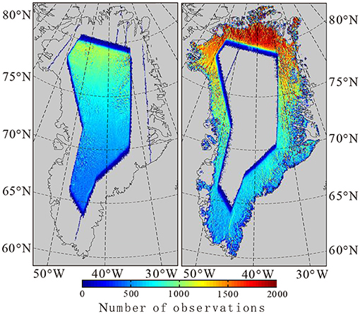
Figure 1. Data distribution of CryoSat-2 LRM mode (Left) and SARin mode (Right). Different colors stand for the number of observations for each 5-km × 5-km grid.

Operation IceBridge Airborne Topographic Mapper Data

The Airborne Topographic Mapper (ATM) is a scanning laser altimeter used in the Operation IceBridge airborne mission operated by the National Aeronautics and Space Administration (NASA). It can measure surface elevation changes in the polar ice of the Earth. Combined with ATM data, the record of observations started by ICESat is extended, and multi-satellite altimetry measurements are linked. The mission has been operated every spring in Greenland since 1993. The ATM data provide a valid comparison for CryoSat-2 data, because laser altimeters generally have better accuracy than radar altimeters (Brenner et al., 2007). In this study, we use ATM observations for two purposes: to evaluate the elevation change estimation algorithm for CryoSat-2 measurements and to increase valid observations for GrIS elevation change rate determination. The ATM L4 data from 2010 to 2018, which are provided by National Snow and Ice Data Center (NSIDC) and contain surface elevation change rates derived from overlapping ATM observations, are used. Readers may refer to Studinger (2018) for further details about the ATM L4 product.

Ice, Cloud, and Land Elevation Satellite Data

The Ice, Cloud, and Land Elevation Satellite (ICESat) mission is the first low-Earth-orbit satellite with a specific laser altimeter onboard and is launched by NASA. It operated 18 33-day campaigns from 2003 to 2009 and provided important information for volume loss in the GrIS during that period. The elevation and volume changes in the GrIS between 2003 and 2009 are estimated using the ICESat data and compared with the results from between 2010 and 2019. In this study, the GLA12-release 34 products provided by NSIDC are used.

Methods for Elevation Change Estimation

Elevation Difference Method for CryoSat-2 Synthetic Aperture Interferometric Mode and Airborne Topographic Mapper Data

In the existing studies, the surface fit method was widely used for surface elevation change determination from CryoSat-2 (Helm et al., 2014; McMillan et al., 2016; Nilsson et al., 2016; Simonsen and Sørensen, 2017; Sørensen et al., 2018). However, this method has limited accuracy on the margins of the ice sheet where undulating terrains appear (see section Validation for CryoSat-2 Derived Result for details). Therefore, an alternative method, referred to as the elevation difference method, is proposed to estimate the elevation change rates on the peripheries of the GrIS. This method eliminates spatially varying elevation differences before the elevation change rates are estimated, so that these two parts can be solved separately. Here, the elevation difference, ΔH(Δt), can be defined as

where H(t_i) and H(t_j) are two elevation observations at exactly the same location obtained at different times t_i and t_j. Considering long-term and seasonal elevation changes, each elevation observation can be expressed as

where dH/dt is the long-term elevation change rate, H₀ is the reference elevation at reference time t₀, and s₁ and s₂ are coefficients of the trigonometric functions used to fit the seasonal elevation change. For CryoSat-2 SARin observations, the impact of changing scattering properties of the ice sheet surface should also be considered, because changing snow penetration depth has a significant effect on radar altimetry observations (Slater et al., 2019; Otosaka et al., 2020). To alleviate this impact, a backscatter correction factor is applied following Simonsen and Sørensen (2017). Consequently, dBs in Equation (2) is the elevation variation caused by backscatter changes, Bs(t) is the surface backscatter at time (t), and $\stackrel{-}{B}s$ is the mean backscatter. Considering Equations (1) and (2), the elevation difference can be written as

In a small region, a consistent elevation change pattern is assumed (Nilsson et al., 2016), and long-term elevation change rate can be estimated by least squares estimation of Equation (3).

No slope corrections are considered in Equation (3), since elevation difference should be derived from observations at exactly the same position. Therefore, the derivation of elevation differences is crucial for this method. For SARin observations, the elevation difference determination is illustrated in Figure 2. Squares and black dots represent measurements from two adjacent SARin tracks, i and j, respectively. Note that the footprints of the SARin data are not necessarily located in a straight line like in conventional altimeters but may be more scattered. Then, the elevation difference is calculated as follows:

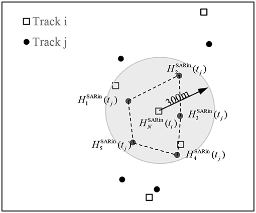
Figure 2. Illustration of the elevation difference method. Squares and black dots represent measurements from track i and track j, respectively. The gray circle shows the 300-m search window and the dashed polygon shows the boundary of the interpolation area.

a. For observations from track i, $H_N^{\mathrm{\text{SARin}}}(t_i)$, measured at time (t_i), the nearby observations from another track (e.g., track j) within 300 m from $H_N^{\mathrm{\text{SARin}}}(t_i)$ (the gray circle in Figure 2) is selected for the next step, denoted as $H_1^{\mathrm{\text{SARin}}}(t_j),\cdots ,H_n^{\mathrm{\text{SARin}}}(t_j)$. However, if there is less than three observations from track j within the 300-m radius search window, this track will be skipped, and observations from another nearby track will be checked.

b. At the exact same position of $H_N^{\mathrm{\text{SARin}}}(t_i)$, an interpolated elevation at time (t_j), denoted as H_{int er}(t_j), can be obtained by bilinear interpolation of the observations selected from track j [e.g., $H_1^{\mathrm{\text{SARin}}}(t_j),\cdots ,H_n^{\mathrm{\text{SARin}}}(t_j)$]. To ensure reliable accuracy, interpolation is only carried out when $H_N^{\mathrm{\text{SARin}}}(t_i)$ is located inside the polygon formed by $H_1^{\mathrm{\text{SARin}}}(t_j),\cdots ,H_n^{\mathrm{\text{SARin}}}(t_j)$ (i.e., dashed lines in Figure 2).

c. The elevation difference measurement is determined as the difference of $H_N^{\mathrm{\text{SARin}}}(t_i)$ and H_{int er}(t_j):

The surface elevation change rate given in the ATM L4 data is simply determined by the division of elevation difference and time difference from overlapping ATM observations (Studinger, 2018). To make the spatial resolution and time span of the ATM data consistent with CryoSat-2, the elevation change rates from ATM L4 are recalculated using the elevation difference method. The elevation difference of each pair of overlapping observations can be restored:

where ΔH_ATM is the elevation difference, and Ḣ_ATM and Δt_ATM are elevation change rate and time difference given in the ATM L4 product. Generally, no seasonal variations would be detected by ATM, because all the observations used in the L4 product were operated in spring. Snow penetration also does not need to be considered for laser altimeter like ATM. Hence, the average elevation change rate can be expressed as:

Equation (6) can be regarded as a special form of Equation (3). Finally, the surface elevation change rates are calculated in 5-km × 5-km grids following McMillan et al. (2016). In order to remove unreliable observations, the mean and standard deviation σ of residuals in each grid is calculated, and a 3σ iterative convergent edit is used.

Surface Fit Method for CryoSat-2 Low Resolution Mode Data

The surface fit method has been proved to be a better way for CryoSat-2 data than the crossover method used for conventional LRM observations (Nilsson et al., 2016). In this study, we apply this method for CryoSat-2 LRM data. The surface fit method is performed by fitting a linear model to the elevations as a function of time and space inside a relatively small area under the assumption that elevation changes are consistent in the area. In addition, a backscatter correction factor is applied to alleviate the impact of changing scattering properties of the ice sheet surface (Simonsen and Sørensen, 2017). Hence, CryoSat-2 measurements can be expressed as follows:

In Equation (7), the ground surface is fitted by the cubic polynomial, where a₀ ~ a₉ are coefficients, and (x,y) and (x₀,y₀) are coordinates of measurement and center of the calculation area, respectively. Other symbols have the same meaning as those in Equations (2)–(4). The parameters can be estimated by least squares estimation. Same as the elevation difference method, elevation changes are calculated in 5-km × 5-km grids, and the 3σ iterative convergent edit is used to remove the outliers.

Elevation Change Algorithms for Ice, Cloud, and Land Elevation Satellite

To estimate the 2003–2009 surface elevation change rate of the GrIS, a repeat track analysis similar to Zwally et al. (2011) is applied for the ICESat data from 17 campaigns (L2a–L2f, L3a–L3k). The repeated tracks were divided into 500-m segments. In each segment, a reference track is selected, and measurements are interpolated to equally spaced (172 m) reference points along each track. Then, the interpolated point $H_i^{ICESat}$ can be denoted as:

where H₀ and t₀ are elevation and observation time of the reference point, k is the surface slope at cross track direction, and D_i is the cross track distance to the reference track. The rest of the characters are similar to those in Equation (2). Further details can be found in Zwally et al. (2011) and Chen and Zhang (2019). The equations are solved in each segment and then gridded into 5-km × 5-km grids by Kriging interpolation.

Validation for CryoSat-2 Derived Result

While laser altimetry data have been proved to be reliable in the GrIS (Krabill et al., 2002; Brenner et al., 2007; Schenk and Csathó, 2012; Csatho et al., 2014; Brunt et al., 2017), the elevation change rates derived from the CryoSat-2 data should be verified, and the effectiveness of the new method adopted for the SARin-covered area should also be tested. In this section, the results of elevation changes derived from the CryoSat-2 data are compared with those from ATM for validation. For SARin observations, both the surface fit and elevation difference methods are investigated and compared. For LRM observations, the effectiveness of the surface fit method is tested. Since only the ATM L4 product between 2010 and 2018 is available online at the time of the study, the time range of CryoSat-2 observations used in this section is also limited from July 2010 to June 2018 to make the two datasets more comparable.

The results derived from ATM and CryoSat-2 are shown in Figure 3. Comparing the two methods used for the SARin-covered area (Figures 3c,d), similar trends are mostly found, while remarkable differences occur at the edge of the GrIS, especially over the southeast coastal region. Extensive positive elevation change rates are found using the surface-fit method in those areas, while moderate negative changes are found using the elevation difference method. However, a recent study that used the combination of Gravity Recovery and Climate Experiment (GRACE) satellite and surface mass balance data showed mass loss at the southeast margin of the GrIS (Wang et al., 2019), which is contradictory to the results of the surface fit method but consistent with those of the elevation difference method. Comparison with ATM also suggests that the elevation difference method is better than the surface fit method. The difference between elevation change rates derived from CryoSat-2 and ATM (defined as CryoSat-2—ATM) is shown in Figure 4. In the difference map of the surface-fit method and ATM (Figure 4a), the red spots at the margin of the GrIS indicate a serious underestimation of elevation decline for the CryoSat-2 result. In contrast, the difference between the elevation difference method and ATM (Figure 4b) shows much better results in general, and improvement in the southeast coastal area is quite obvious.

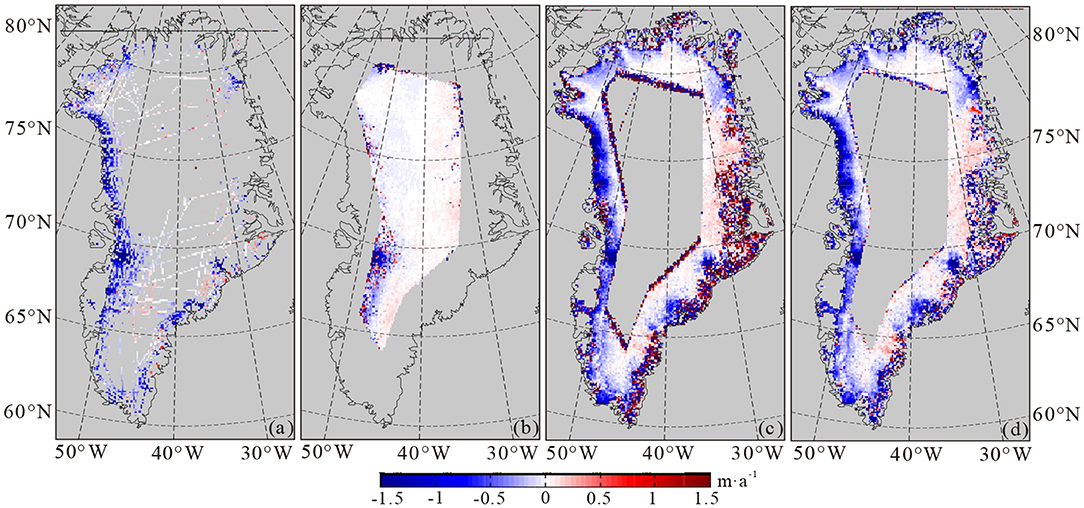
Figure 3. Elevation changes in 2010–2018 derived from (a) ATM L4 data, (b) CryoSat-2 LRM data, (c) CryoSat-2 SARin data calculated by the surface fit method, and (d) CryoSat-2 SARin data calculated by the elevation difference method.

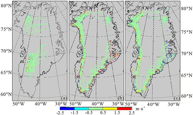
Figure 4. Elevation change rate difference of (a) Figures 3a,b, (b) Figures 3a–c, and (c) Figures 3a–d.

For further discussion, the differences shown in Figure 4 are analyzed statistically. All the elevation change rate differences greater than ±10 m·a⁻¹ are considered to be outliers. By this criterion, 470 outliers are removed for the surface fit method, and 69 are removed for elevation fitting. Since the two methods reveal similar results in the flat inland area but different results in the undulating marginal area, surface slope is further considered in statistics. Therefore, an ICESat-derived digital elevation model (DEM) of the GrIS (DiMarzio, 2007) provided by NSIDC is used to determine the surface slope in each grid. For the entire SARin-covered area, about 9,500 grids are compared with ATM for both methods. The differences between the results derived from SARin and ATM are classified according to the surface slope. The mean and standard deviation (SD) of the differences and the number of grids used for statistics in each surface slope category are shown in Table 1. Surface slope has a great impact on the surface fit method, but it has less effect on the elevation difference method. In flat areas with a surface slope of <0.2°, the two methods have almost the same mean difference of about 3 cm·a⁻¹ compared to ATM, with a difference of only 0.1 mm·a⁻¹. With the increase in surface slope, the average difference between the surface fit method and ATM increases rapidly and reaches 1.492 ± 3.639 m·a⁻¹ when the surface slope is more than 1°. By comparison, the mean differences between the elevation difference method and ATM seem to be random with the increase in surface slope. The mean differences are generally centimeter-scale, except for the case when the surface slope is more than 1°, but the value of −0.359 is still considerably better than the case of the surface fit method. The new method also shows a lower standard deviation than that of the surface fit method in all surface slope classifications. While the elevation difference method reveals results similar to those of ATM in the entire area with an average difference of 0.017 ± 1.128 m·a⁻¹, the surface fit method is not so reliable with an obvious bias of +25.24 cm·a⁻¹ and a greater standard deviation of ±1.854 m·a⁻¹. Generally, the results shown in Table 1 suggest that the elevation difference method is better than the surface fit method in determining the surface elevation change rate of areas with a high slope. We suggest that this discrepancy can be attributed to the different strategies used for topographic correction. The details are discussed in section Impact of Topography for the Surface Fit Method.

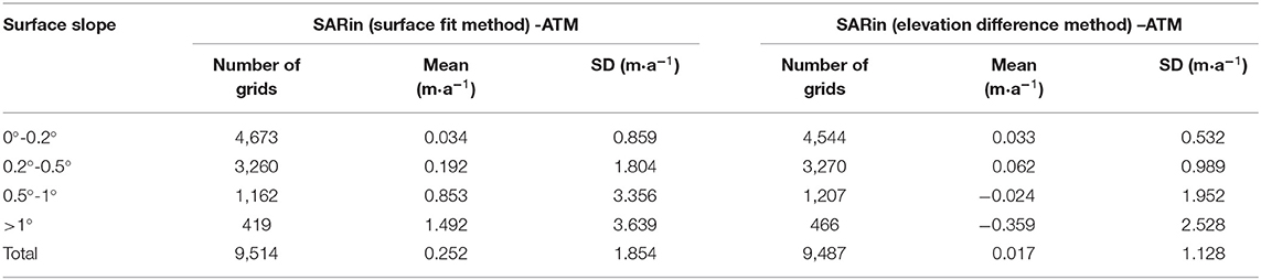
Table 1. Differences in ice sheet elevation changes obtained by CryoSat-2, SARin, and ATM observations.

The results in Table 1 also show that the surface-fit method has little difference with the elevation difference method when the surface slope is low. Hence, only the surface fit method is used for LRM data, because LRM is only operated at the flat and smooth areas in the interior of the GrIS. The elevation changes derived from LRM are shown in Figure 3b, and their differences with ATM are shown in Figure 4a. Again, the grids with elevation change rate difference greater than ±10 m·a⁻¹ are removed as outliers, and 3,485 grids remain for the comparison. The mean difference of the two data sets is 0.01 m·a⁻¹, with a standard deviation of 0.878 m·a⁻¹, which indicates that the results of the LRM process are reliable.

Results

Greenland Ice Sheet Elevation Change Between 2010 and 2019

Although the elevation difference method generally shows reasonable results, a small proportion of biased grids in the SARin-covered area still exists and can be distinguished, as shown in Figure 4 (e.g., Jakobshavn Isbræ around 50°W, 69°N). Therefore, a further combination of the SARin and ATM data is adopted to improve the accuracy in the SARin-covered area based on the elevation difference method. For the LRM-covered area, the ATM data are not involved, because they are in good agreement with the LRM data. Hence, the results in this area are determined only by the LRM data with the surface fit method.

With the procedures mentioned above, the CryoSat-2 Level 2 product from July 2010 to July 2019 and the ATM L4 product from 2010 to 2018 are used for the final results. The elevation change rates are calculated in regular 5-km × 5-km grids. Grids with an root mean square (RMS) larger than 0.5 m·a⁻¹ from least squares estimation are rejected as outliers. Considering the characteristics of elevation changes in the GrIS in recent decades (Nilsson et al., 2015), the grids with an elevation change rate either larger than +3 m·a⁻¹ or smaller than −15 m·a⁻¹ are also considered to be outliers. The blanks between altimetry tracks are filled by Kriging interpolation to cover the entire GrIS drainage systems given by Zwally et al. (2012). Following Nilsson et al. (2016), the uncertainty of the elevation change rate in each 5-km × 5-km grid is basically determined from the standard deviations of the differences between CryoSat-2 and ATM. However, different from Nilsson et al. (2016), the uncertainties used in this study are not only distinguished by observation modes (i.e., LRM and SARin) but also by surface slope according to the classification shown in Table 1. Our final result for the GrIS surface elevation change from 2010 to 2019 is given in Figure 5. The average elevation change rate for the entire GrIS is −11.83 ± 1.14 cm·a⁻¹, equivalent to a volume loss of −200.22 ± 18.26 km³·a⁻¹. The negative numbers indicate that the GrIS is still in a state of obvious mass loss as a whole after 2010. In Figure 5, the boundaries of eight drainage systems (DSs 1–8) and 19 sub-drainage systems (DSs 1.1–8.2), according to Zwally et al. (2012), are shown in gray lines, and the 2,000-m elevation contour line is also presented as the black solid line.

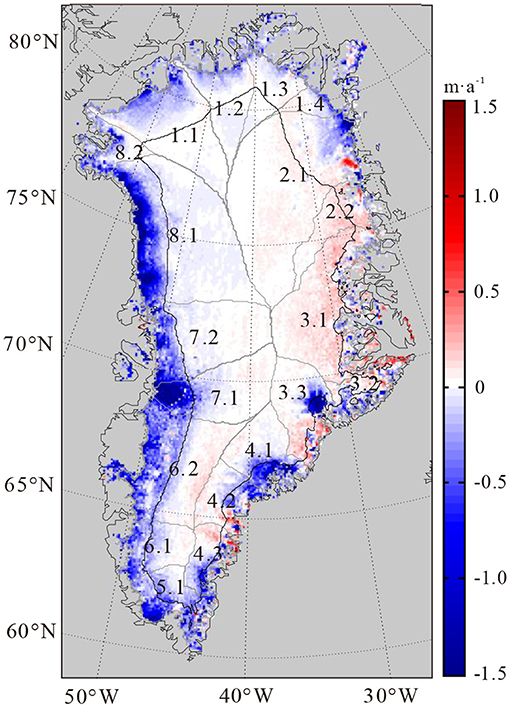
Figure 5. Distribution of elevation change rates in the Greenland ice sheet from 2010 to 2019. The black solid line is the 2,000-m elevation contour. The gray lines and the numbers show the boundaries and locations of different drainages.

As shown in Figure 5, relatively stable conditions from 2010 to 2019 can be seen in the interior of the GrIS (i.e., above 2,000 m elevation), and rapid elevation decline can be found on the margins of the ice sheet, especially at the northwest coast in DS 8.1, Jakobshavn Isbræ in DS7.1, and several large coastal outlet glaciers in DS3.3 and DS4. Extreme elevation changes below −10 m·a⁻¹ occur in some grids at the regions mentioned above. Areas above 2,000 m had a slight rise in elevation with a change rate of +1.12 cm·a⁻¹, equivalent to a volume change rate of +12.10 km³·a⁻¹. Elevation and volume changes in each drainage system are shown in Table 2.

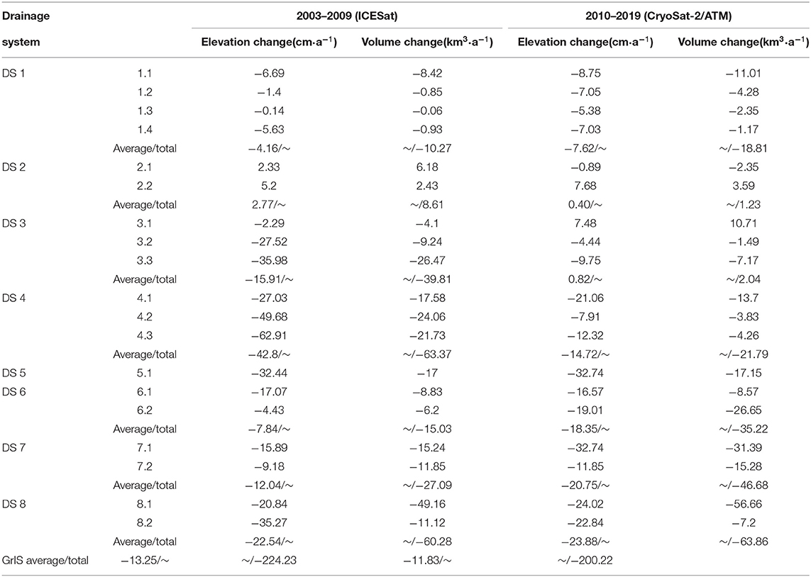
Table 2. Elevation and volume changes in each drainage system for different time periods.

Greenland Ice Sheet Elevation Change Comparison: 2003–2009 vs. 2010–2019

To further understand the elevation and volume changes in the GrIS, the results from 2010 to 2019 obtained from CryoSat-2 and ATM data are compared with the results derived from ICESat between 2003 and 2009. The average volume loss rate derived from ICESat is −224 ± 15 km³·a⁻¹, which is a comparable result compared with existing studies (Sørensen et al., 2011; Ewert et al., 2012). The results are shown in Figure 6. For simplicity of expression, the two periods will be mentioned as period I (2003–2009) and period II (2010–2019) hereafter. Figure 6b shows the difference between the results from the two periods (periods II and I). During the period I, the glaciers in southeast Greenland were undergoing severe volume loss (Howat et al., 2008), but moderate elevation changes were found during period II (see Figure 5). Negative values can be found during both periods in southwest coastal areas, while the speed of elevation decline had accelerated in Period II, indicating more serious deglaciation. This fact can be confirmed by the blue zones at the southwest part of the GrIS, as shown in Figure 6b. On the other hand, although negative elevation change rates appear in both periods, Figure 6b shows remarkable red zones in DS 3 and DS 4, indicating an obvious slowdown in the speed of glacier ablation in the east coastal region during period II compared with period I. Most areas in the interior GrIS have slightly negative values as well, indicating potential ablations in high elevation areas.

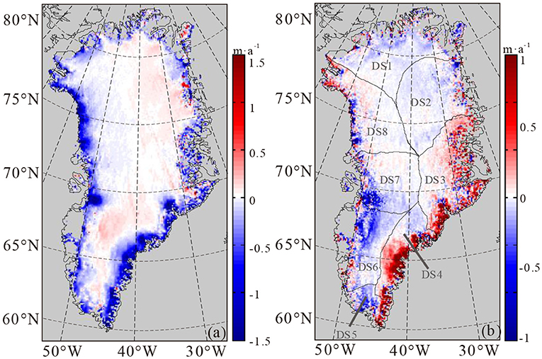
Figure 6. (a) Elevation change derived from ICESat (2003–2009) and (b) difference between (a) and Figure 5.

Elevation and volume change rates during the two periods in each single drainage and sub-drainage systems are given in Table 2. The volume loss during period II is −200.22 km³·a⁻¹ for the entire GrIS, about 24 km³·a⁻¹ less than the value during period I, showing a remission in snow and ice loss. For both periods, DS 8 showed a sustained severe volume loss of around −60 km³·a⁻¹, which was the fastest among the eight drainage systems during Period I, and the second fastest during Period II. Considering a negligible difference of only 3.6 km³·a⁻¹ for the two different periods, DS 8 is regarded to be the drainage system with the most serious glacier loss. The volume change rate in DS 5 of about −17 km³·a⁻¹ does not seem to be conspicuous because of the small area of this drainage, but the elevation change rate of this drainage system is eye-catching. The values are over −32 cm·a⁻¹ in DS 5 for both periods, which is the second fastest elevation change rate during period I and the fastest during period II. DS 4 has both fastest elevation and volume change rate among the ICESat derived results, but great alleviation of about +41.6 km³·a⁻¹ in volume change rate occurred during Period II (−63.37 km³·a⁻¹ for period I vs. −21.79 km³·a⁻¹ for period II). DS 3 is undergoing similar changes as DS 4, where the variation of volume change rate over time is also over +40 km³·a⁻¹ (−39.81 km³·a⁻¹ for period I vs. +2.04 km³·a⁻¹ for period II). Howat et al. (2008) reported astonishing volume losses in DSs 3 and 4 due to mass losses in numerous marine-terminating outlet glaciers along the coast. However, as shown in Figure 5, no obvious volume loss can be found in DSs 3 and 4, except for the two large glaciers, Kangerdlugssuaq in DS 3.3 and Helheim in DS 4.1. The elevation and volume change rates of four other drainages (DSs 1, 2, 6, and 7) are all lower during Period II than during Period I, indicating acceleration in volume loss (DSs 1, 6, and 7) or deceleration in volume growth (DS 2).

Discussion

Impact of Penetration Depth of CryoSat-2 Radar Altimetry

Variation in penetration depth into the snow surface is a typical disadvantage of the application of CryoSat-2 in the GrIS. Previous research studies have shown that the penetration depth in a dry snow zone can achieve several meters (Slater et al., 2019) and that abrupt changes were shown when an extreme melting event occurs (Nilsson et al., 2015; Slater et al., 2019; Otosaka et al., 2020). Although the actual impact of penetration on elevation observations is greatly mitigated by retracking algorithms, it might still lead to a deviation from radar altimeter-derived elevation changes (Gray et al., 2019; Otosaka et al., 2020). To assess whether the CryoSat-2 derived elevation change is affected by radar penetration, the GrIS elevation change between 2010 and 2019 was further estimated by CryoSat-2 observations from four summer months (June, July, August, and September) and compared with the result of CryoSat-2 observations from all 12 months. The difference is shown in Figure 7. The elevation change estimated by summer observations is considered to be less affected by radar penetration, because radar returns are predominantly from the melted snow surface (Gray et al., 2019). If the snow penetration does have an obvious influence on the long-term elevation change estimation of the GrIS, the difference between the two results should be easily distinguished. However, no significant spatial pattern is shown in Figure 7, which means that the penetration has little impact on the estimation. The scattered random differences are more likely due to the reduced number of observations in the summer months. After removing the outliers by a 3σ edit, the average difference of the two results is −0.003 ± 0.323 m·a⁻¹ for LRM and −0.003 ± 0.58 m·a⁻¹ for SARin. The accordance between CryoSat-2 and ATM described in section Validation for CryoSat-2 Derived Result also suggests that reliable elevation changes can be captured by CryoSat-2. This result agrees with the conclusion of Slater et al. (2019) that the impact of snow penetration on derived elevation trend becomes negligible over a long time period.

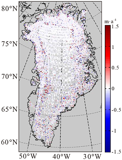
Figure 7. Differences in elevation changes derived from CryoSat-2 summer (June to September) and all-year-round observations.

Impact of Topography for the Surface Fit Method

In general, the elevation change results in coastal regions are poorer than the interior because the precision and accuracy of radar altimetry observations are limited by surface slope. However, the surface fit method is much more affected by surface slope than the elevation difference method, as shown in Figure 3 and Table 1. Two sample 5-km × 5-km grids, located in 68°02′N, 33°48′W (referred to as sample grid 1) and 67°57′N, 50°00′W (referred to as sample grid 2) separately, were further investigated to find out why the surface fit method is so vulnerable to undulating terrains. Both grids are located on the margins of the GrIS and have a surface slope of over 1°. The distribution of observed elevations, simulated terrain according to Equation (7), the elevation residuals, and observation time are shown in Figure 8. For sample grid 1, it is shown that the cubic polynomial in Equation (7) failed to fit the actual topography properly, because obvious spatial patterns can still be seen in the residuals (Figure 8c). The results of sample grid 2 are even worse, because the simulated terrain (Figure 8f) is not similar to the observed terrain (Figure 8e) at all, and the residual will be absorbed into the time-related elevation changes. Then, we tested different surface fitting functions for the two sample grids, from plane fit (1st-order function) to 5th-order-surface fit, and the results are shown in Table 3, together with the results of the elevation difference method and ATM. Considering the deviation from the ATM results, the complexity of the fitting function used in the surface fit method has limited improvement. The reason for this crucial mistake happening is probably because the time-varying elevation changes and spatially varying elevation differences are hard to be separated in Equation (7) in complex terrains. However, in both sample grids, the elevation difference method has shown much better accordance with ATM. For the elevation difference method, the impact of topography is alleviated by spatial interpolation. Hence, the elevation change can be resolved separately with reliable performance. We also divided the two sample grids into 2.5-km × 2.5-km grids to find out if a smaller region can be beneficial to the surface fit method. For sample grid 1, the results of the four smaller grids are determined to be 0, 0.612, −0.598, and −0.307 m·a⁻¹. For sample grid 2, the results are 5.057, 3.872, 0.414, and 2.921 m·a⁻¹. All these results did not seem to be in accordance with ATM observations. In theory, a smaller region should be easier to be fitted by polynomial functions, but we did not test a much smaller grid size, because the number of observations would also be reduced.

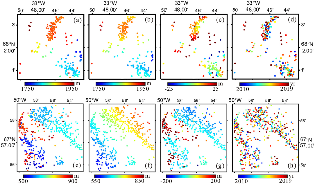
Figure 8. Distribution of (a) observed elevations, (b) simulated elevations according to Equation (7), (c) residuals of simulated terrain, and (d) observation time from sample grid 1. (e–h) are same as (a–d) but from sample grid 2.

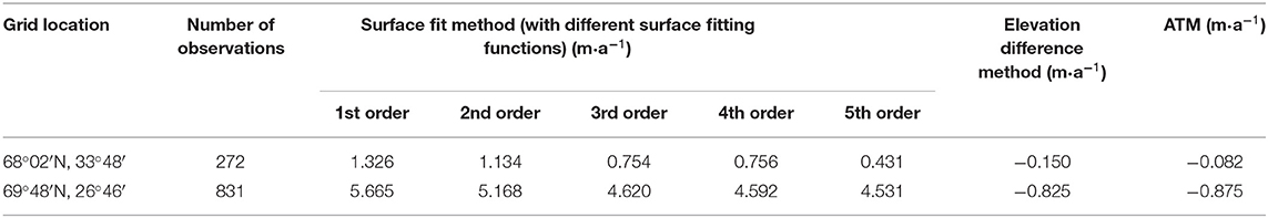
Table 3. Elevation change rates in the two sample grids calculated in different ways.

Abrupt Deceleration in GrIS Deglaciation

Bevis et al. (2019) reported an abrupt slowdown in deglaciation, referred to as the “2013–2014 Pause,” during the period of 2013–2014 observed by the Greenland GPS Network and the GRACE satellite mission. The “Pause” was also confirmed by altimetry data. Since laser altimeters have several advantages compared with radar altimeters, the time series of ATM observations are used to study the “2013–2014 Pause.” As shown in Figures 9, 10, selected 5-km × 5-km grids from different drainages, named as grids a–j, generate their corresponding time series. For each grid, the elevation of 2010 is set to 0 as a reference, and the elevation difference from the ATM L4 product is used to obtain the relative elevation of the 2010 reference by the least-squares estimation. Linear trends are fitted for two stages: the pre-Pause stage from 2010 to 2013 and the post-Pause stage from 2013 to 2018. If the relative elevation of 2013 is missed because of the absence of ATM observation, the two stages are separated by the year 2014 instead. The resulting time series and linear trends are shown in Figure 9 for each grid.

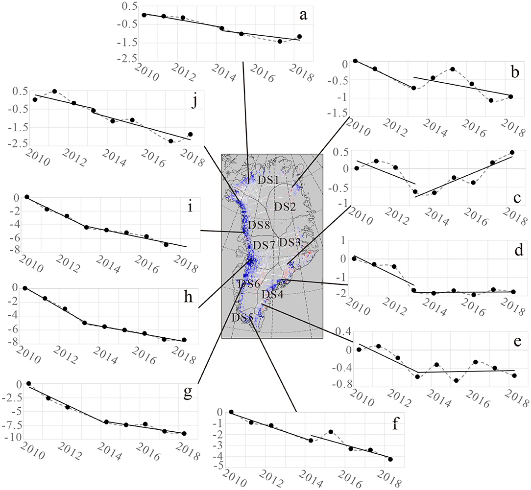
Figure 9. Time series of elevation in selected grids (a–j) based on ATM observations. Black dots and dashed lines represent the time series in each selected grids. Black solid lines in each diagram show the elevation trend before and after the “Pause”.

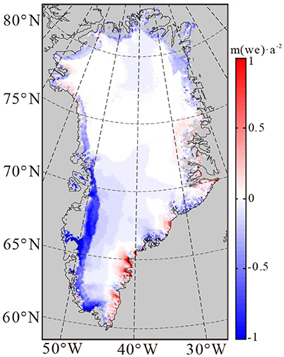
Figure 10. Difference between averaged SMB of 2003–2009 and 2010–2019.

A clear slowdown can be seen by comparing the linear trends of the pre- and post-Pause stages in most of the selected grids, except for grids a and j in the northwest Greenland and grid f in the southern part, providing obvious evidence for the “2013–2014 Pause.” Results from grids c, d, and e (representing DSs 3 and 4) matched well with the values shown in Table 2 and show most evident alleviation in elevation decline. The linear trends for grids g, h, and i (representing DSs 6, 7, and the southern part of DS 8) also show alleviation in elevation decline, while the results shown in Table 2 indicate acceleration after 2010. This seeming contradiction reflects the fact that the volume loss in this area during 2010–2014 is far more serious than the situation during 2003–2009, so that the average change rate of 2010–2019 stays low even if deceleration happened after 2014. This conclusion can be confirmed by the volume change rate of −375 km³·a⁻¹ during 2011–2014 derived from CryoSat-2 (Helm et al., 2014), which showed a considerable faster volume loss rate than the results of −224 km³·a⁻¹ for 2003–2009 and −200 km³·a⁻¹ for 2010–2019 given in this study. In general, grids a, g, h, i, and j, located in western Greenland, show stable trends during the post-Pause stage, while alternating elevation rise and fall take place in grids b, c, d, and e, located in the eastern part. Nevertheless, the “2013–2014 Pause” is obviously detected by ATM observations, and its effect was still continuing in 2018.

Reduced Glacier Mass Loss in Southeast GrIS

In the first decade of the twenty-first century, massive ice loss due to intensive marine-terminating outlet glaciers was found in southeast and northwest GrIS (Howat et al., 2008; Kjeldsen et al., 2013). The situation in the southeast coast shifted dramatically into a moderate elevation decline during the 2010–2019 period (see Figure 5 and Table 2). As the main contributor of GrIS mass loss in recent years (Zhang et al., 2019; Sasgen et al., 2020), SMB (surface mass balance) from the regional climate model RACMO2.3p2 (Noël et al., 2019) is considered for further discussion. Figure 10 shows the difference between the average SMB for periods I and II mentioned in section Greenland Ice Sheet Elevation Change Comparison: 2003–2009 vs. 2010–2019. For most of the areas, Figure 10 shows similar trends compared with Figure 6b. Discrepancies are obviously revealed in the southeast coastal region. While the elevation decline in Figure 6a shows apparent attenuation in the whole area, moderate enhancements in SMB are partially detected. This discrepancy indicates that the alleviation of elevation decline in the southeast part should be attributed to the reduction in dynamic ice loss of the marine-terminating outlet glaciers. Since the ice discharge from marine-terminating outlet glaciers is greatly affected by the ocean (Bevis et al., 2019; Khazendar et al., 2019), it is a proof that the impact of oceanic force on this area is weakening. However, the alternating elevation rise and fall in grids c, d, and e after 2012, shown in Figure 9, reflects the complexity of the mixed impact of the oceanic and atmospheric forces. Once the oceanic force was recovered, the volume loss in the southeast part might be intense again.

Conclusions

One of the most important objectives of this study is to determine the elevation and volume change rates in the GrIS during the 2010–2019 period from altimetry data. The method of surface elevation change rate determination with CryoSat-2 data is discussed. The surface fit method is selected for LRM data, and an elevation difference method is proposed for the SARin data. Through validation with ATM data, the elevation difference method has obvious advantages in constraining the impact of undulating terrains at the margins of the ice sheet. The final result of 2010–2019 GrIS elevation changes is derived from the combination of CryoSat-2 and ATM data to achieve better accuracy. The average elevation and volume change rates are −11.83 ± 1.14 cm·a⁻¹ and −200.22 ± 18.26 km³·a⁻¹, respectively.

Another objective of this study is to compare the elevation/volume change in the GrIS for the 2010–2019 period with the results from the 2003–2009 period to investigate the trend in deglaciation in recent years. The result of −224 ± 15 km³·a⁻¹ derived from ICES at laser altimetry for 2003–2009 was about 10% faster than the result from CryoSat-2 and ATM. This comparison indicated alleviation in volume loss during 2010–2019. The elevation decline in the southeast coast of the GrIS has a considerably large scale of recovery, while the situation of volume loss in the west margin is getting worse. This phenomenon indicates that the impact of the ocean on the GrIS has been weakened, and that the major source of deglaciation is transferring from the southeast coast to the west margin of the ice sheet.

Further analysis was carried out for the time series of ATM data for selected representative grids in each drainage system. The results clearly demonstrate the “2013–2014 Pause” reported by Bevis et al. (2019), and its effect did not seem to end by 2018. However, the “Pause” had different effects on different regions according to the ATM time series. In general, the west margin of the GrIS had shown stable trends after the “Pause,” while complex variations had appeared on the eastern coast.

The elevation and volume changes in the GrIS in recent years seem to be complex, and further research studies are necessary for investigating the ice loss in different drainages and time periods. Better accuracy of altimetry data is, thus, required. The CryoSat-2 Level-2 GDR data used in this study still suffer from several problems, e.g., scattering properties of the reflecting surface, phase ambiguities in the SARin data (Abulaitijiang et al., 2015), and poor accuracy in slope terrains. These problems are expected to be partly or mostly solved by adopting specialized retracking algorithms and phase ambiguity corrections on the basis of Level-1b data. In addition, the incorporation of observations from new generation altimetry missions (e.g., ICESat-2) can improve the results as well. The study on new data processing and strategy for joint calculation from multi-source data is still undergoing.

Data Availability Statement

The raw data supporting the conclusions of this article will be made available by the authors, without undue reservation.

Author Contributions

GC and SZ contributed to conception and design of the study. GC and JZ organized the database. GC and SL performed the statistical analysis. GC wrote the first draft of the manuscript. SZ wrote sections of the manuscript. All authors contributed to manuscript revision, read, and approved the submitted version.

Funding

This study was supported by the Basic Research Program of Jiangsu Province (No. BK20180973), the National Natural Science Foundation of China (No. 41804002), and the Open Research Foundation of the Key Laboratory of Geospace Environment and Geodesy, the Ministry of Education, Wuhan University (No. 19-01-04).

Conflict of Interest

The authors declare that the research was conducted in the absence of any commercial or financial relationships that could be construed as a potential conflict of interest.

Acknowledgments

The authors would like to thank Prof. Jonathan Bamber for providing the 1-km Greenland surface type grid, Prof. H. Jay Zwally for providing Greenland drainage system boundaries, and Dr. Brice Noël for providing SMB from RACMO2.3p2. The authors would also like to thank ESA for providing CryoSat-2 products, and NSIDC for providing ICESat, ICESat-2, and ATM products and Greenland DEM. The authors would also like to thank the two reviewers who provided constructive comments that helped improve the manuscript.

References

Abulaitijiang, A., Andersen, O. B., and Stenseng, L. (2015). Coastal sea level from inland CryoSat-2 interferometric SAR altimetry. Geophys. Res. Lett. 42, 1841–1847. doi: 10.1002/2015GL063131
Bamber, J. L., Griggs, J. A., Hurkmans, R. T. W. L., Dowdeswell, J. A., Gogineni, S. P., Howat, I., et al. (2013). A new bed elevation dataset for Greenland. Cryosphere 7, 499–510. doi: 10.5194/tc-7-499-2013
Bevis, M., Harig, C., Khan, S. A., Brown, A., Simons, F. J., Willis, M., et al. (2019). Accelerating changes in ice mass within Greenland, and the ice sheet's sensitivity to atmospheric forcing. Proc. Natl. Acad. Sci. U.S.A. 116, 1934–1939. doi: 10.1073/pnas.1806562116
Brenner, A. C., DiMarzio, J. P., and Zwally, H. J. (2007). Precision and accuracy of satellite radar and laser altimeter data over the continental ice sheets. IEEE Transac. Geosci. Remote Sens. 45, 321–331. doi: 10.1109/TGRS.2006.887172
Brunt, K. M., Hawley, R. L., Lutz, E. R., Studinger, M., Sonntag, J. G., Hofton, M. A., et al. (2017). Assessment of NASA airborne laser altimetry data using ground-based GPS data near Summit Station, Greenland. Cryosphere 11, 681–692. doi: 10.5194/tc-11-681-2017
Cao, B., Pan, B., Guan, W., Wang, W., and Wen, Z. (2017). Changes in ice volume of the Ningchan No. 1 Glacier, China, from 1972 to 2014 as derived from in situ measurements. J. Glaciol. 63, 1025–1033. doi: 10.1017/jog.2017.70
Chen, G., and Zhang, S. (2019). Elevation and volume change determination of Greenland Ice Sheet based on icesat observations. Chin. J. Geophys. 62, 2417–2428. doi: 10.6038/cjg2019M0170
Church, J. A., Clark, P. U., Cazenave, A., Gregory, J. M., Jevrejeva, S., Levermann, A., et al. (2013). “Sea level change,” in Climate Change 2013: The Physical Science Basis. Contribution of Working Group I to the Fifth Assessment Report of the Intergovernmental Panel on Climate Change, eds T. F. Stocker, D. Qin, G. K. Plattner, M. Tignor, S. K.Allen, J. Boschung, A. Nauels, Y. Xia, V. Bex, and P. M. Midgley (Cambridge: Cambridge University Press), 1137–1216. doi: 10.1017/CBO9781107415324.026
Csatho, B. M., Schenk, A. F., Veen, C. J. V. D., Babonis, G., Duncan, K., Rezvanbehbahani, S., et al. (2014). Laser altimetry reveals complex pattern of Greenland Ice Sheet dynamics. Proc. Natl. Acad. Sci. U.S.A. 111, 18478–18483. doi: 10.1073/pnas.1411680112
DiMarzio, J. P. (2007). GLAS/ICESat 1 km Laser Altimetry Digital Elevation Model of Greenland. Available online at: https://nsidc.org/data/NSIDC-0305/versions/1 (accessed May 7, 2021).
Ewert, H., Popov, S. V., Richter, A., Schwabe, J., Scheinert, M., and Dietrich, R. (2012). Precise analysis of ICESat altimetry data and assessment of the hydrostatic equilibrium for subglacial Lake Vostok, East Antarctica. Geophys. J. Int. 191, 557–568. doi: 10.1111/j.1365-246X.2012.05649.x
Gardner, A. S., Moholdt, G., Cogley, J. G., Wouters, B., Arendt, A. A., Wahr, J., et al. (2013). A reconciled estimate of glacier contributions to sea level rise: 2003 to 2009. Science 340, 852–857. doi: 10.1126/science.1234532
Gray, L., Burgess, D., Copland, L., Langley, K., Gogineni, P., Paden, J., et al. (2019). Measuring height change around the periphery of the Greenland Ice Sheet with radar altimetry. Front. Earth Sci. 7:146. doi: 10.3389/feart.2019.00146
Helm, V., Humbert, A., and Miller, H. (2014). Elevation and elevation change of Greenland and Antarctica derived from CryoSat-2. Cryosphere 8, 1539–1559. doi: 10.5194/tc-8-1539-2014
Howat, I. M., Smith, B. E., Joughin, I., and Scambos, T. A. (2008). Rates of southeast Greenland ice volume loss from combined ICESat and ASTER observations. Geophys. Res. Lett. 35:L17505. doi: 10.1029/2008GL034496
Khazendar, A., Fenty, I. G., Carroll, D., Gardner, A., Lee, C. M., Fukumori, I., et al. (2019). Interruption of two decades of Jakobshavn Isbræ acceleration and thinning as regional ocean cools. Nat. Geosci. 12, 277–283. doi: 10.1038/s41561-019-0329-3
Khvorostovsky, K. S. (2012). Merging and analysis of elevation time series over Greenland Ice Sheet from satellite radar altimetry. IEEE Transac. Geosci. Remote Sens. 50, 23–36. doi: 10.1109/TGRS.2011.2160071
Kjeldsen, K. K., Khan, S. A., Wahr, J., Korsgaard, N. J., Kjær, K. H., Bjørk, A. A., et al. (2013). Improved ice loss estimate of the northwestern Greenland Ice Sheet. J. Geophys. Res. Solid Earth 118, 698–708. doi: 10.1029/2012JB009684
Krabill, W. B., Abdalati, W., Frederick, E. B., Manizade, S. S., Martin, C. F., Sonntag, J. G., et al. (2002). Aircraft laser altimetry measurement of elevation changes of the Greenland Ice Sheet: technique and accuracy assessment. J. Geodynam. 34, 357–376. doi: 10.1016/S0264-3707(02)00040-6
Levinsen, J. F., Khvorostovsky, K., Ticconi, F., Shepherd, A., Forsberg, R., Sørensen, L. S., et al. (2015). ESA ice sheet CCI: derivation of the optimal method for surface elevation change detection of the Greenland Ice Sheet – round robin results. Int. J. Remote Sens. 36, 551–573. doi: 10.1080/01431161.2014.999385
McMillan, M., Leeson, A., Shepherd, A., Briggs, K., Armitage, T., Hogg, A., et al. (2016). A high-resolution record of Greenland mass balance. Geophys. Res. Lett. 43, 7002–7010. doi: 10.1002/2016GL069666
Muhammad, S., and Tian, L. (2016). Changes in the ablation zones of glaciers in the western Himalaya and the Karakoram between 1972 and 2015. Remote Sens. Environ. 187, 505–512. doi: 10.1016/j.rse.2016.10.034
Muhammad, S., Tian, L., and Khan, A. (2019). Early twenty-first century glacier mass losses in the Indus Basin constrained by density assumptions. J. Hydrol. 574, 467–475. doi: 10.1016/j.jhydrol.2019.04.057
Nilsson, J., Gardner, A., Sørensen, L. S., and Forsberg, R. (2016). Improved retrieval of land ice topography from CryoSat-2 data and its impact for volume-change estimation of the Greenland Ice Sheet. Cryosphere 10, 2953–2969. doi: 10.5194/tc-10-2953-2016
Nilsson, J., Vallelonga, P., Simonsen, S. B., Sørensen, L. S., Forsberg, R., Dahl-Jensen, D., et al. (2015). Greenland 2012 melt event effects on CryoSat-2 radar altimetry. Geophys. Res. Lett. 42, 3919–3926. doi: 10.1002/2015GL063296
Noël, B., van de Berg, W. J., Lhermitte, S., and van den Broeke, M. R. (2019). Rapid ablation zone expansion amplifies north Greenland mass loss. Sci. Adv. 5:eaaw0123. doi: 10.1126/sciadv.aaw0123
Otosaka, I. N., Shepherd, A., Casal, T. G., Coccia, A., Davidson, M., Di Bella, A., et al. (2020). Surface melting drives fluctuations in airborne radar penetration in West Central Greenland. Geophys. Res. Lett. 47:e2020GL088293. doi: 10.1029/2020GL088293
Pritchard, H. D., Arthern, R. J., Vaughan, D. G., and Edwards, L. A. (2009). Extensive dynamic thinning on the margins of the Greenland and Antarctic ice sheets. Nature 461, 971–975. doi: 10.1038/nature08471
Sasgen, I., Wouters, B., Gardner, A. S., King, M. D., Tedesco, M., Landerer, F. W., et al. (2020). Return to rapid ice loss in Greenland and record loss in 2019 detected by the GRACE-FO satellites. Commun. Earth Environ. 1:8. doi: 10.1038/s43247-020-0010-1
Schenk, T., and Csathó, B. (2012). A new methodology for detecting ice sheet surface elevation changes from laser altimetry data. IEEE Trans. Geosci. Remote Sens. 50, 3302–3316. doi: 10.1109/TGRS.2011.2182357
Shepherd, A., Ivins, E. R., Geruo, A., Barletta, V. R., Bentley, M. J., Bettadpur, S., et al. (2012). A reconciled estimate of ice-sheet mass balance. Science 338, 1183–1189. doi: 10.1126/science.1228102
Simonsen, S. B., and Sørensen, L. S. (2017). Implications of changing scattering properties on Greenland Ice Sheet volume change from Cryosat-2 altimetry. Remote Sens. Environ. 190, 207–216. doi: 10.1016/j.rse.2016.12.012
Slater, T., Shepherd, A., McMillan, M., Armitage, T., Otosaka, I., and Arthern, R. (2019). Compensating changes in the penetration depth of pulse-limited radar altimetry over the Greenland Ice Sheet. IEEE Transac. Geosci. Remote Sens. 57, 9633–9642. doi: 10.1109/TGRS.2019.2928232
Sørensen, L. S., Simonsen, S. B., Forsberg, R., Khvorostovsky, K., Meister, R., and Engdahl, M. (2018). 25 years of elevation changes of the Greenland Ice Sheet from ERS, Envisat, and CryoSat-2 radar altimetry. Earth Planet. Sci. Lett. 495, 234–241. doi: 10.1016/j.epsl.2018.05.015
Sørensen, L. S., Simonsen, S. B., Nielsen, K., Lucas-Picher, P., Spada, G., Adalgeirsdottir, G., et al. (2011). Mass balance of the Greenland Ice Sheet (2003–2008) from ICESat data – the impact of interpolation, sampling and firn density. Cryosphere 5, 173–186. doi: 10.5194/tc-5-173-2011
Studinger, M. (2018). IceBridge ATM L4 Surface Elevation Rate of Change, Version 1. Available online at: https://nsidc.org/data/IDHDT4/versions/1?qt-data_set_tabs=4#qt-data_set_tabs (accessed May 7, 2021).
The IMBIE Team (2019). Mass balance of the Greenland Ice Sheet from 1992 to 2018. Nature 579, 233–239. doi: 10.1038/s41586-019-1855-2
Thomas, R., Davis, C., Frederick, E., Krabill, W., Li, Y., Manizade, S., et al. (2008). A comparison of Greenland ice-sheet volume changes derived from altimetry measurements. J. Glaciol. 54, 203–212. doi: 10.3189/002214308784886225
Velicogna, I., Mohajerani, Y., Landerer, F., Mouginot, J., Noel, B., Rignot, E., et al. (2020). Continuity of Ice Sheet mass loss in greenland and antarctica from the GRACE and GRACE follow-on missions. Geophys. Res. Lett. 47:e2020GL087291. doi: 10.1029/2020GL087291
Wang, L., Khan, S. A., Bevis, M., van den Broeke, M. R., Kaban, M. K., Thomas, M., et al. (2019). Downscaling GRACE predictions of the crustal response to the present-day mass changes in Greenland. J. Geophys. Res. Solid Earth 124, 5134–5152. doi: 10.1029/2018JB016883
Wang, X., and Holland, D. M. (2018). A method to calculate elevation-change rate of Jakobshavn Isbræ using operation icebridge airborne topographic mapper data. IEEE Geosci. Remote Sens. Lett. 15, 981–985. doi: 10.1109/LGRS.2018.2828417
Zhang, B., Liu, L., Khan, S. A., van Dam, T., Bjørk, A. A., Peings, Y., et al. (2019). Geodetic and model data reveal different spatio-temporal patterns of transient mass changes over Greenland from 2007 to 2017. Earth Planet. Sci. Lett. 515, 154–163. doi: 10.1016/j.epsl.2019.03.028
Zwally, H. J., Giovinetto, M. B., Beckley, M. A., and Saba, J. L. (2012). Antarctic and Greenland Drainage Systems. Available at https://earth.gsfc.nasa.gov/cryo/data/polar-altimetry/antarctic-and-greenland-drainage-systems (accessed May 7, 2021).
Zwally, H. J., Giovinetto, M. B., Li, J., Cornejo, H. G., Beckley, M., Brenner, A. C., et al. (2005). Mass changes of the Greenland and Antarctic ice its sheets and shelves and contributions to sea-level rise: 1992–2002. J. Glaciol. 51, 509–527. doi: 10.3189/172756505781829007
Keywords: altimetry, Greenland ice sheet, Arctic, volume loss, elevation change
Citation: Chen G, Zhang S, Liang S and Zhu J (2021) Elevation and Volume Changes in Greenland Ice Sheet From 2010 to 2019 Derived From Altimetry Data. Front. Earth Sci. 9:674983. doi: 10.3389/feart.2021.674983
Received: 02 March 2021; Accepted: 26 April 2021;
Published: 26 May 2021.
Edited by:
Jinyun Guo, Shandong University of Science and Technology, ChinaReviewed by:
Haihong Wang, Wuhan University, ChinaWan Xiaoyun, China University of Geosciences, China
Copyright © 2021 Chen, Zhang, Liang and Zhu. This is an open-access article distributed under the terms of the Creative Commons Attribution License (CC BY). The use, distribution or reproduction in other forums is permitted, provided the original author(s) and the copyright owner(s) are credited and that the original publication in this journal is cited, in accordance with accepted academic practice. No use, distribution or reproduction is permitted which does not comply with these terms.
*Correspondence: Guodong Chen, cgdtt@126.com; Shengjun Zhang, zhangshengjun@mail.neu.edu.cn