Seismogenic Structure Orientation and Stress Field of the Gargano Promontory (Southern Italy) From Microseismicity Analysis

Introduction

The high seismicity rate of the Italian territory periodically causes serious damage and human losses. The investigation of active tectonic structures is of fundamental importance for the mitigation of the seismic risk. An improvement in the knowledge is then required to gain further insights on the seismogenic structures of the area. In particular, the seismogenic structures of the Gargano Promontory (hereafter GP) are still under discussion; the peculiar geographical position of the GP, the long recurrence time for large earthquakes, and the poor instrumental coverage by the RSN are the main causes for the delay in the knowledge of this seismic sector. Geodynamically, the GP and the Apulia region are considered to belong to the Adriatic microplate or Adria plate (Anderson and Jackson, 1987; Figure 1A). This microplate seems to be originated as a result of the split-up of the old collision boundaries (McKenzie, 1972; Favali et al., 1990) and played an important role in this geodynamical context, being considered as the foreland of the Alps, Apennine, and Dinarides (Di Bucci and Angeloni, 2013).

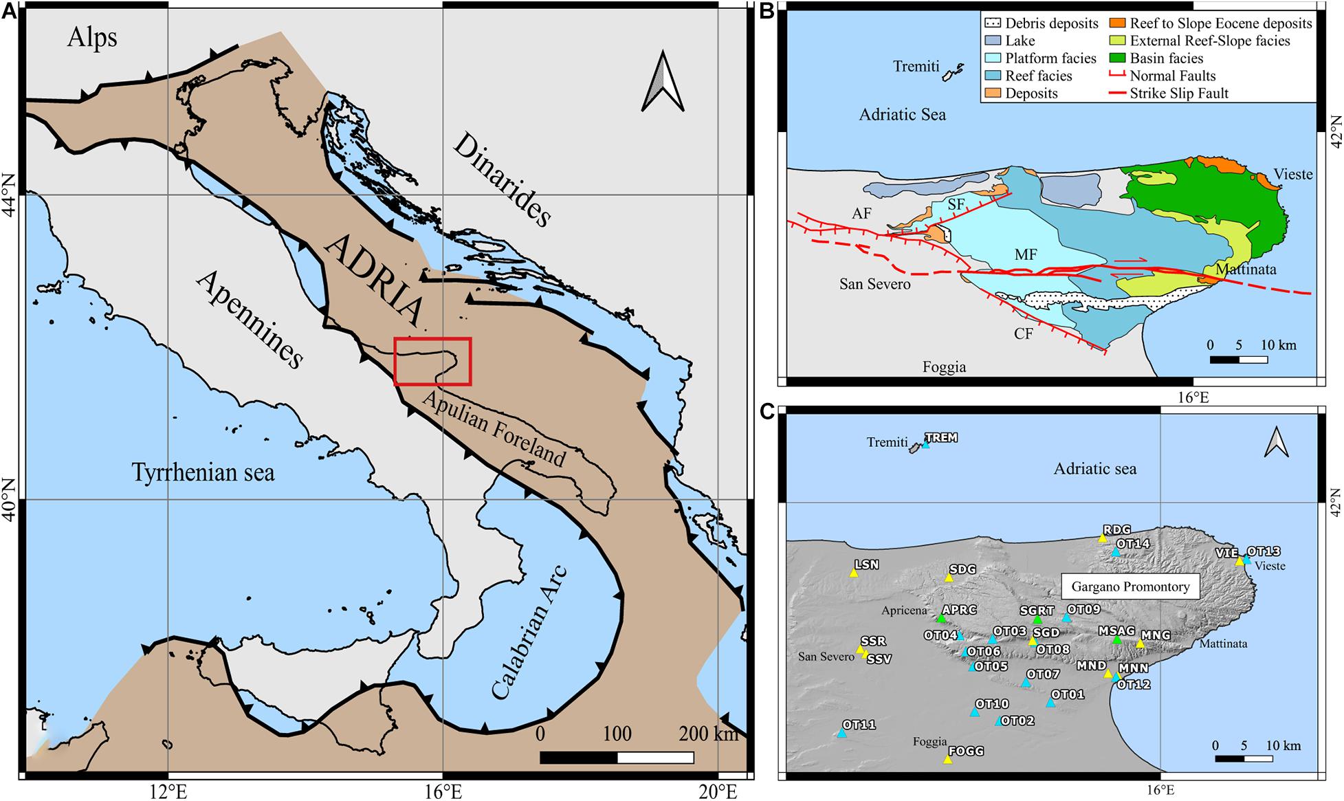
Figure 1. (A) Adria microplate (brown area) as reported by Mantovani et al. (2006). The red square indicates the area investigated in this paper. (B) Simplified geological map. The main stratigraphical and geological features are reported (Salvi et al., 1999; Chilovi et al., 2000; Bosellini and Morsilli, 2001; Patacca and Scandone, 2004); colors of the stratigraphic units refer to the ages of geological formations: Jurassic facies, light blue; Cretaceous facies, green; Eocene facies, orange. We reported in the map the Mattinata Fault (MF), the Apricena Fault (AF), the Candelaro Fault (CF), and the Sannicandro Fault (SF) as red lines, both continuous (that is observable on the ground surface) and discontinuous (that is hypothesized under the ground surface) and their dipping direction. (C) Enlargement on the red area of GP. The triangles refer to different seismic networks according to colors: green refers to RSN; light blue refers to OSN; yellow refers to National Accelerometric Network (RAN) managed by the Civil Protection Department (DPC).

The GP represents the highest sector of the Apulian foreland (around 1,000 m above the sea level) that extends to the East toward the Adriatic Sea (Figure 1B) and is mainly composed by slightly deformed carbonatic successions (Del Gaudio et al., 2007) as shown in the geological map in Figure 1B, where the main stratigraphical and geological features are reported. Based on previous geological maps (Bosellini and Morsilli, 2001; Cotecchia, 2014), we reported the main stratigraphical units of the area according to the typical depositional profile of the carbonate environment. Concerning the tectonic structures, many faults are recognized along the entire GP. However, the characteristics of these structures are poorly known. This is the reason why we included in the tectonic map only the main structures for which some information can be found: the Mattinata Fault (MF) (Chilovi et al., 2000), the Apricena Fault (AF) (Patacca and Scandone, 2004), the Candelaro Fault (CF) (Mongelli and Ricchetti, 1970), and the Sannicandro Fault (SF) (Salvi et al., 1999) as red lines.

The GP tectonic evolution is rather complex and is a topic of debate. Although many authors agree that the MF (Figure 1B) is the main structure involved in the development of the GP sector, its kinematics is controversial. Many authors reported that MF had a left-lateral strike-slip kinematics (Funiciello et al., 1988; Salvini et al., 1999), but several researchers considered the hypothesis of a reactivation with right-lateral motion during the late Pliocene until today (Chilovi et al., 2000; Tondi et al., 2005). In contrast, many other authors have always considered this structure as a right-lateral strike-slip structure (Piccardi, 1998). According to these authors, this structure was active since its first activation, recognized in lower Cretaceous (Piccardi, 1998), as confirmed also by the 2002 Molise earthquake (Valensise et al., 2004; Piccardi, 2005). Other studies ascribed the evolution of this area to a system of parallel E-W faults that border the promontory to the North and South (with the MF system) generating compressive stress (Brankman and Aydin, 2004) or that split this area promoting a general uplift linked to the high subduction angle of the Adria microplate (Doglioni et al., 1994). Recent results from the stress field inversion show active tectonics currently characterized by a compressive regime, with a NW-SE dominant shortening according to the NE-SW minimum horizontal stress axis orientation (Montone and Mariucci, 2016). Evidence of compression was also reported offshore, as inferred from the analysis of seismic profiles (Argnani et al., 1993, 2009; Scisciani and Calamita, 2009) and onshore with the study of well logs and geological data (Bertotti et al., 1999).

The GP and surrounding regions have been hit by several strong earthquakes, as the 1627 (Mw = 6.7 ± 0.1), the May 31, 1646 (Mw = 6.7 ± 0.3), and the March 20, 1731 (Mw = 6.3 ± 0.1) earthquakes (Rovida et al., 2019). All these historical earthquakes have an estimated magnitude larger than six. In the period 1985–2013, the RSN recorded a lot of microearthquakes in the GP (de Lorenzo et al., 2017), despite the small number of seismometers located in the area. Since 2013, cooperation between the University of Bari, the INGV (National Institute of Geophysics and Volcanology), and the INFN (National Institute of Nuclear Physics) in the frame of the OTRIONS project (Tallarico, 2013) allowed a further improvement in the seismic coverage of the area, with the installation of 12 new seismic stations (Filippucci et al., 2021a). Since then, a large number of microearthquakes have been recorded. This allowed us to gain several important geophysical results for this area.

In particular, de Lorenzo et al. (2017) collected the first earthquake database by using the recordings of the network stations in the period 2013–2014 and developed a 1D velocity model for GP. Furthermore, by using the same earthquake database, the rheological behavior of GP crust (Filippucci et al., 2019a), the level of energy absorption (Filippucci et al., 2019b), and the stress field (Filippucci et al., 2020) were analyzed. In 2015, the network geometry was updated: some stations were switched off, and other stations were added in the northern part of GP, allowing a better seismic coverage and a less azimuthal gap of the recorded earthquakes. In this paper, we added to this dataset the earthquakes recorded in the period from 2015 to 2020. The earthquake seismic recordings of the period 2013–2018 were recently released on the Mendeley data repository (Filippucci et al., 2021b); the earthquakes recorded in the period 2019–2020 can be found on the EIDA platform. In this paper, using a more robust earthquake database, we extended the region of interest moving to the northern sector of the GP and tried to find the relationships between the known fault structures and the present-day microseismicity of this area. Finally, we retrieve the stress field using first-motion polarities focal mechanisms.

Materials and Methods

Seismic Database

The OTRIONS Seismic Network (OSN) (Figure 1C) is operating in the GP and Capitanata area since April 2013. The OSN stations are integrated, in real time, with those of the RSN (Figure 1C). During the first 6 years of OSN operation, a high number of microearthquakes, below the magnitude of minimum detection of the RSN, were recorded even if the event detection was affected by several problems of data transmission and archiving (Filippucci et al., 2021a). During the first 15 months of operation, a manual work of event detection was done (de Lorenzo et al., 2017). Since July 2014 to the end of 2018, the event detection was demanded to the SeisComP3 software (Helmholtz Centre Potsdam GFZ German Research Centre for Geosciences and gempa GmbH, 2008) with manual picking revision. Waveform data from 2013 to 2018, with picking times marked, were recently released (Filippucci et al., 2021b). From the beginning of 2019 to the present day, data are archived and distributed by INGV-EIDA. The waveforms were downloaded from the EIDA archive, and the picking was manually revised. Furthermore, for the period 2019–2020, seismic data were integrated with data from the National Accelerometric Network (RAN) (Figure 1C). Since these instruments operate with a triggering system, the recordings are not available for all the events, but, where possible, the azimuthal gap was significantly reduced, and the number of available first motion polarities was increased.

The collected events constitute a database of 1,894 microearthquakes. All the collected events were relocated using Hypo71 (Lee and Lahr, 1972) and a 1D velocity model computed for GP (de Lorenzo et al., 2017). Station corrections have been included in the analysis as computed by de Lorenzo et al. (2017). Hypo71 was run with different starting depths, in order to better explore the parameter space. The best location for each event was selected minimizing the following dimensionless parameter S (Michele, 2016):

where RMS is the computed root mean square, RMS₀ = 1 s is a reference residual time, ERH is the horizontal error of the estimated hypocenter, ERZ is the vertical error, d_min is the minimum source to the receiver distance, and Z is the foci depth. The network sensitivity allowed us to record thousand events. Earthquakes belonging to neighboring zones were discarded due to the high azimuthal gap, θ. We also recorded very small events, clustered around some active quarries and probably due to quarry explosions, which we removed from our database. Because of the GP geographical position, it is difficult to obtain earthquake location with θ less than 180°, especially for the events located along the coastline and offshore. For this reason, we considered acceptable all the solutions with θ < 240°. We also discarded all the solutions with RMS greater than 0.5 s. This selection process led us to reduce the database to 635 events, mapped in Figure 2 and listed in Supplementary Table 1. The quality of the database is described in Figure 3, where the frequency histograms of ERZ and ERH and the histogram of the event RMS are shown. The 99% of hypocenter locations have errors within 5 km; in particular, 93.5% of the horizontal errors and 92.4% of the vertical errors are less than 2 km, with an average horizontal error of 0.55 km and an average vertical error of 0.60 km; 73% of the residuals are less than 0.2 s with an average of 0.2 s. These histograms indicate the high quality of the localizations. Therefore, an update of the velocity model is not necessary.

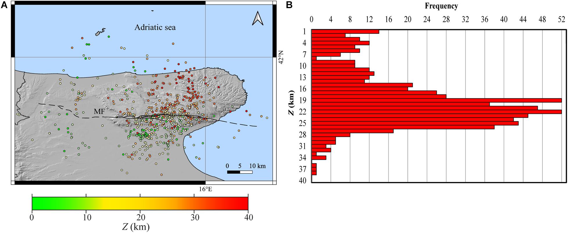
Figure 2. (A) Epicenters of the 635 microearthquakes recorded between April 2013 and June 2020 and listed in Supplementary Table 1. Different colors refer to depth as indicated in the color scale bar; (B) Frequency histogram of the hypocenters.

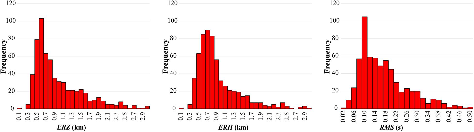
Figure 3. Frequency histograms of the vertical (ERZ) and horizontal (ERH) localization errors and of the event RMS for all the 635 events recorded from April 2013 to June 2020.

Since December 2018, we estimated the vertical local magnitude (Mlv); from January 2019, the horizontal local magnitude (Ml) was considered as computed by INGV. The two major events recorded in the analyzed period are the April 23, 2017 with Mlv = 4.0 and the April 18, 2020 with Ml = 3.7 (respectively, ID = 333 and ID = 602, Supplementary Table 1). In particular, Mlv ranges between 0.1 and 2.8 and Ml ranges between 0.5 and 3.6 with the 90% of both Ml and Mlv < 2.0 (Supplementary Table 1).

Focal Mechanism Determination

We used the FocMec code (Snoke et al., 1984) to retrieve focal mechanisms from the inversion of P-wave first-motion polarities. Since we deal with earthquakes of magnitude from very low to low, the number of available polarities is very low too. Starting from a database of 635 earthquakes, we selected a total of 200 earthquakes having a minimum number of six P-wave polarities data to compute focal mechanisms.

We carried out several tests with different weights attributed to the polarity data. The FocMec code allows us to assign an error for each discrepant polarity observation according to the weight conditions imposed by the user (Snoke, 2017). Considering the small number of P-wave polarity data for each event of our database, the best choice consists of assigning a unity-weighting equal to zero; this choice is the most restrictive, since only fault plane solutions (FPS) without discrepant polarities can be accepted by the code. For each event, the code returns all the FPS compatible with the polarity data. In some cases, the acceptable FPS are so different that we cannot uniquely identify the best one, and the event must be discarded. In Figure 4, we show an example of accepted and discarded FPS, and all the 36 accepted focal mechanisms.

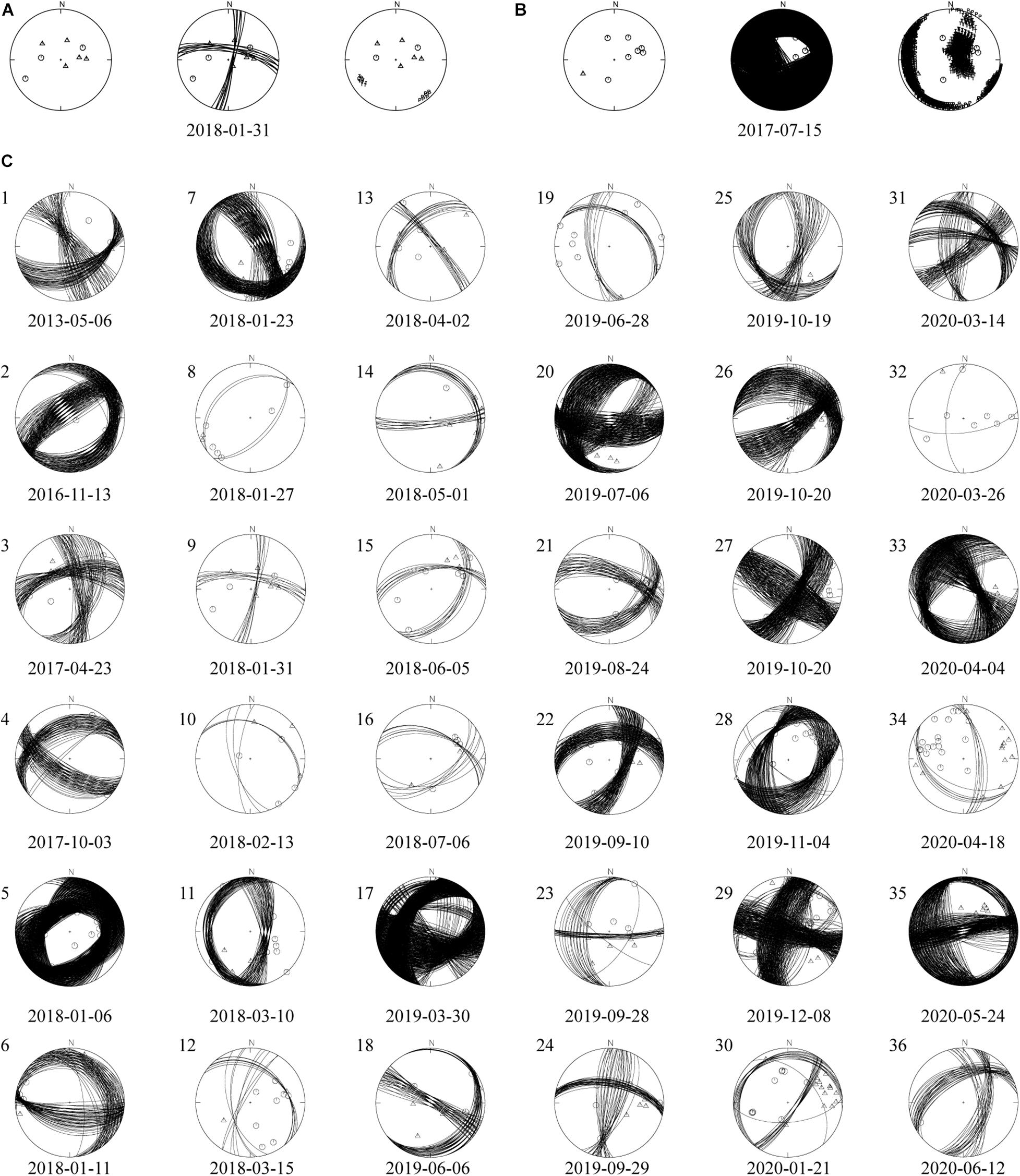
Figure 4. FocMec solutions: (A) Example of an accepted event solution (case of the January 31, 2018 earthquake); (B) example of a discarded event solution (case of the July 15, 2017 earthquake). From left to right, the P-wave polarity distribution, the fault plane solutions, and the P-T axes distribution are shown in the focal spheres. (C) The 36 accepted focal mechanisms according to the criteria described in the Focal Mechanism Determination section. Dates below the solutions refer to the origin time of the event (Table 1).

Following the approach described by Hardebeck and Shearer (2002), for each event, the average of the inferred fault planes is considered as the preferred one, and the uncertainty is represented by the standard deviation Δϕ, Δδ, and Δλ of strike ϕ, dip δ, and rake λ. FPS is considered constrained only if the set of planes is tightly clustered around the average fault plane. At the end of this procedure, we accepted only solutions with Δϕ, Δδ, and Δλ ≤ 40° simultaneously. By using the above-described criteria, 36 well-constrained focal mechanisms were considered as acceptable. In Table 1, we reported the average value and the standard deviation for ϕ, δ, and λ of the 36 FPS couples (FPS 1 and FPS 2), together with the localization parameters. We also indicated the faulting type (FT) according to the classification of Zoback (1992) in the version modified by Frepoli et al. (2017) (Table 1). The accepted solutions are shown on the GP geographical map both as beachballs (Figure 5A), colored according to FT (Heidbach et al., 2016) and as P-T axes (Figure 5B) sketched according to FT too (Heidbach et al., 2016).

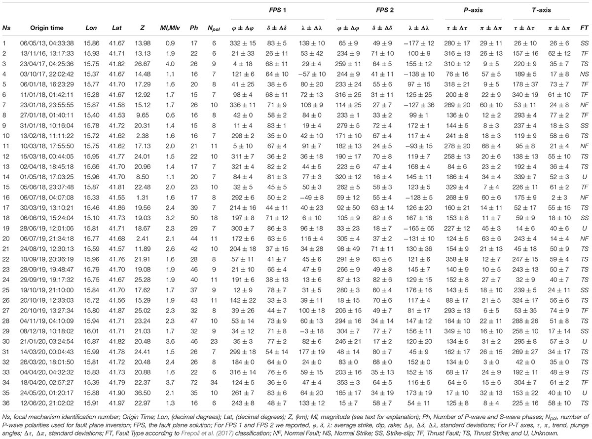
Table 1. List of accepted focal mechanism solutions.

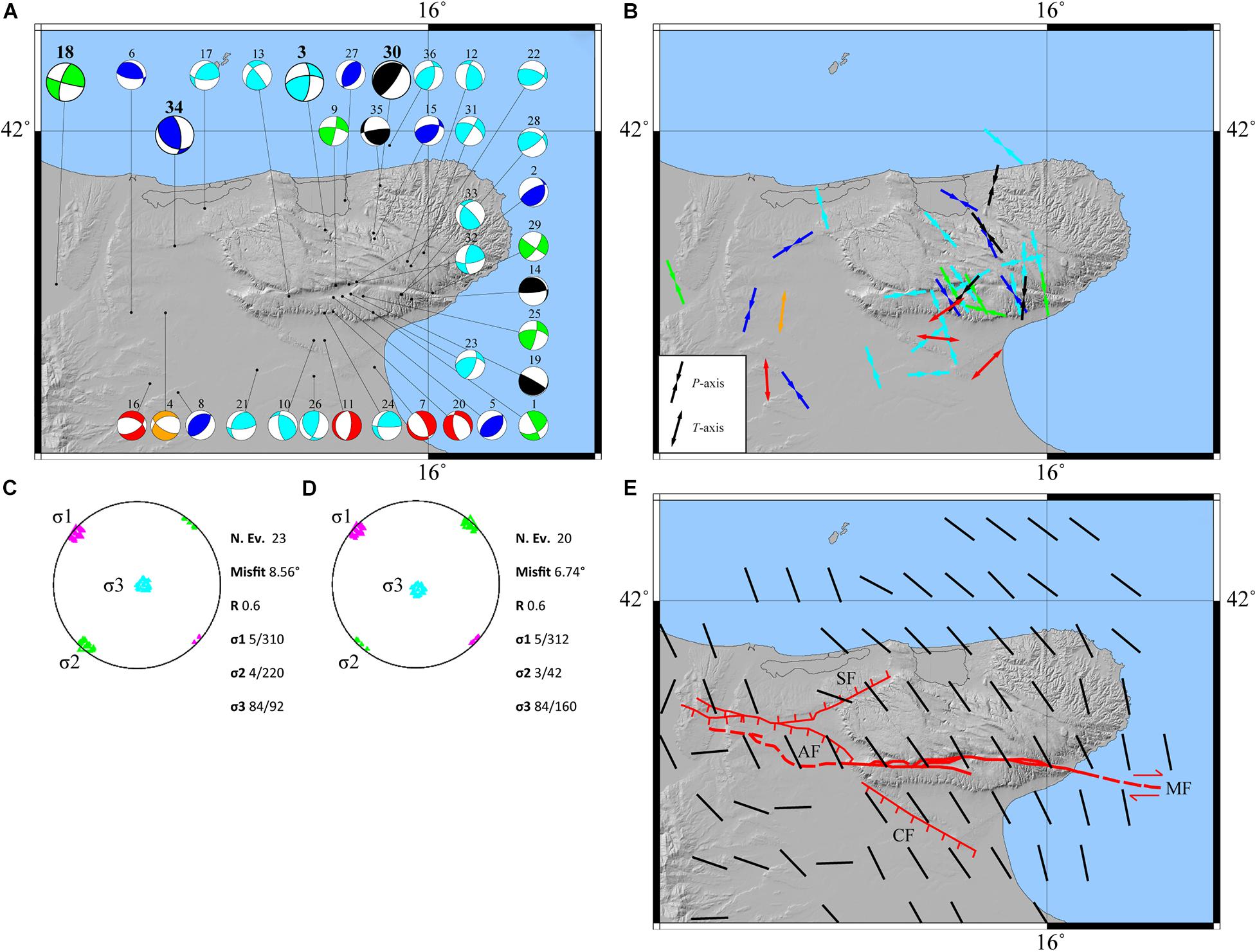
Figure 5. (A) Distribution on map of the 36 average focal mechanisms computed from our data. The different color identifies the kinematics according to the guidelines of the World Stress Map (Heidbach et al., 2016). Red, NF; Orange, NS; Green, SS; Cyan, TS; Blue, TF; Black, U. Focal mechanisms dimensions are scaled according to magnitude ranges (small for Ml < 3; big for Ml ≥ 3). (B) P-T axes distribution and orientation on map. Arrows represent P-T axes and colors refer to the Heidbach et al. (2016). P-axes are reported for TF, TS, SS, and U kinematics, while T-axes are reported for NF and NS kinematics. (C) The stress axis on the stereo-net with confidence regions for each principal stress axis for 23 focal mechanisms; π and τ angles of σ are reported. (D) The same as (C) for 20 focal mechanisms as described in the Error Propagation and Validation section. (E) Stress data interpolation provided with SHINE code (Carafa et al., 2015a). Thick black bars represent the S_Hmax computed by using our 36 focal mechanisms.

Although the S-polarities and amplitude ratios may improve the focal mechanism results, in our case, this improvement is not possible because there are several problems affecting the S-wave data. First of all, the very small magnitude of events reflects into uncertainty that affects the estimated S-wave arrival time: S-wave onset pickings are often associated to a SAC weight from 1 to 3 that corresponds to an uncertainty ranging between 50 and 300 ms. This error bar generally impedes to pick S-polarity. Moreover S-waves are affected by the splitting of the horizontal components. This effect is due to the medium anisotropy. Unfortunately, an anisotropic model of the GP crust is not yet available, and therefore, the S-waves cannot be used to compute the focal mechanisms. In order to use the S-wave information (polarities and amplitudes), it will be therefore necessary to perform a specific study on the anisotropy of GP and Northern Apulia, which is beyond the scope of this paper.

Error Propagation and Validation

The use of a 1D velocity model can bias the earthquake locations, especially in the complex tectonic GP area. In order to account the possible errors induced by the use of the 1D de Lorenzo et al. (2017) velocity model, we relocated the 36 events for which focal mechanisms were computed. We considered the error bar of the velocity model as retrieved by de Lorenzo et al. (2017) and computed a minimum (MIN) and maximum (MAX) velocity model by subtracting and by adding the half-error bar to the central values (AVG), at each depth Z. Then, we recomputed the 36 localizations (Supplementary Table 2). Hypocenters computed with MIN and MAX velocity models are distant from the hypocenter computed with the AVG velocity model, respectively, of 2 and 3 km on average. Epicenters computed with MIN and MAX velocity models are distant from the epicenters computed with the AVG velocity model, respectively, of 1.4 and 1.7 km in horizontal (ED in Supplementary Table 2); foci depths computed with MIN and MAX velocity models are distant from the foci depth computed with the AVG velocity model, respectively, of 1.2 and 2.3 km in vertical (VD in Supplementary Table 2). The distances ED and VD among hypocenters, due to the error bar of the velocity model, are comparable with the localization errors ERH and ERZ (Figure 3).

We also recomputed focal mechanisms by using the three hypocenters for each event (the MIN, the MAX, and the AVG) and plotted the results (Supplementary Figures 1–6). It can be observed that the three focal mechanisms for each event do not show significant variations, indicating stable results. It is worth to note that, since we set FocMec (Snoke et al., 1984) to return only solutions without discrepant polarities, errors in the velocity model can move the polarity to be discrepant and, in some solutions, can be not accepted (Ns = 15, 16, 17, 30, 32, and 34 in Supplementary Figures 3, 5, 6).

The Stress Tensor Inversion

We used the FMSI package (Gephart, 1990) to perform different tests on our focal mechanism database. By performing this inversion, we estimated four of the six components that describe the stress tensor; the three eigenvectors that represents the principal stress direction (σ₁, σ₂, and σ₃, respectively, maximum, intermediate, and minimum compressive stress direction) and the stress ratio, R = (σ₂−σ₁)/(σ₃−σ₁), a dimensionless scalar quantity indicating the shape of the stress tensor.

The data set consists of 36 high-quality focal mechanisms: 7 TF and 15 TS, 4 NF, 1 NS, 5 SS, and 4 U (Figure 5A and Table 1). To constrain the results obtained by the stress tensor inversion, we assigned a weight for each nodal plane. We used the criteria described in Filippucci et al. (2020) and adapted the quality factors of FPFIT (Reasenberg and Oppenheimer, 1985) to the FocMec output. The fitting quality Q_f quantifies how the solution fits polarity data. In this case, all the 36 returned focal mechanisms are perfectly compatible with the polarity observations, so we assigned a default Q_f = 1 to all the events. The nodal plane quality factor Q_p quantifies the quality of the retrieved nodal plane: Q_p = A if (Δϕ, Δδ, Δλ) ≤ 20°; Q_p = B if 20°< (Δϕ, Δδ, Δλ) ≤ 40°, and Q_p = C if (Δϕ, Δδ, Δλ) > 40°. We used the corresponding standard deviation of these three parameters to describe the range of perturbations of △ϕ, △δ, △λ. We assigned Q_p1 = Q_p for FPS 1 and Q_p2 = Q_p for FPS 2, where FPS are the nodal planes identified by FocMec (Table 2). Q_p12 is the total weight assigned to the two FPS: Q_p12 = 3 for the AA class; Q_p12 = 2 for AB, BA, BB, AC classes; Q_p12 = 1 for BC, CB, CA classes was assigned to each event. We also considered the number of polarity data, N_pol, to assign the weight Q_pol to the focal mechanism. Since the number of available observations is very low, we assigned Q_pol = 0 to focal mechanisms computed with N_pol = 6 and N_pol = 7. Then, by scaling for the maximum number of N_pol per event, we assigned the following weights: Q_pol = 1 for 8 ≤ N_pol ≤ 10; Q_pol = 2 for 11 ≤ N_pol ≤ 15; Q_pol = 3 for 16 ≤ N_pol ≤ 20, Q_pol = 4 for 21 ≤ N_pol ≤ 25; Q_pol = 5 for 26 ≤ N_pol ≤ 30; Q_pol = 6 for 31 ≤ N_pol ≤ 35. W_TOT = Q_f + Q_{p12 +} Q_pol is the total weight used in the FMSI inversion for each focal mechanism.

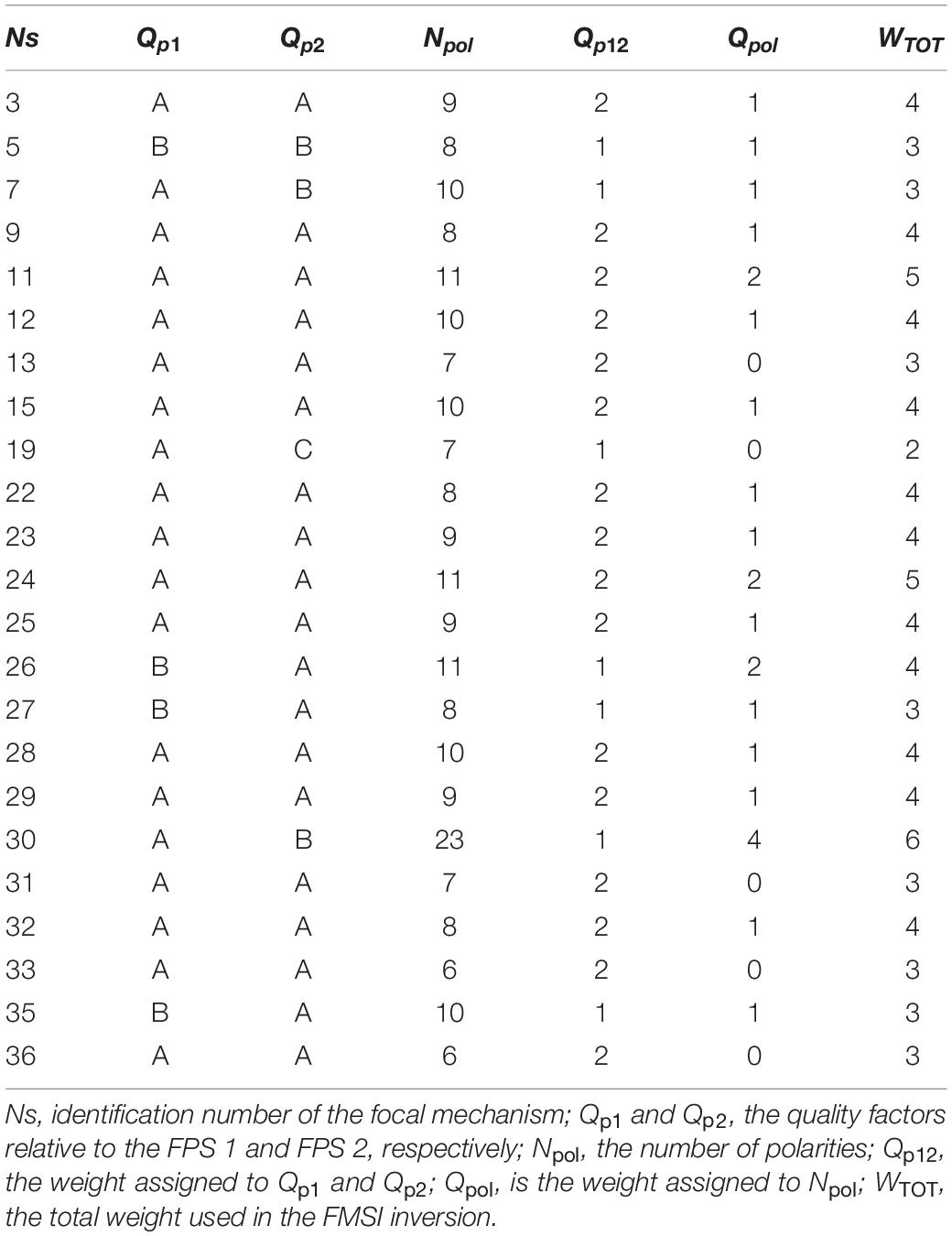
Table 2. Quality classes and assigned weight for the focal mechanisms used in the FMSI inversion.

The frequency histogram of foci depths Z (Figure 2B) shows one main seismogenic layer at 14 < Z < 30 km. Starting from this observation, we grouped focal mechanisms according to depth. A first inversion was performed with 23 events (listed in Table 2), but the misfit angle (Misfit = 8.56° in Figure 5C) was too high to accept this solution, according to the homogeneous criteria proposed by Lu et al. (1997). We then performed a second run by excluding three events (Ns = 7, 11, 26 in Table 2) located borderline of GP. We obtained Misfit = 6.74° (Figure 5D), which indicates a homogeneous compressive stress field with a sub-vertical σ₃ and a maximum horizontal compressive stress, S_Hmax, trending NW-SE according to the Italian Stress Map for GP (Carafa and Barba, 2013; Carafa et al., 2015b; Montone and Mariucci, 2016). The misfit angle (Gephart and Forsyth, 1984) is computed through an angular rotation given by the angular difference between the observed slip direction on a fault plane and the shear stress on that fault plane derived from a given stress tensor; the stress tensor orientation that provides the average minimum misfit is assumed to be the best stress tensor for a given population of focal mechanisms (Frepoli et al., 2011).

Finally, in order to observe the distribution of the stress field within the GP area, we calculated the orientation of S_Hmax (Figure 5E) by interpolating all the 36 focal mechanisms; to this end, we used the method described in Carafa and Barba (2013) and the SHINE code (Carafa et al., 2015a).

Results and Discussion

The seismicity collected in the period from April 2013 to June 2020 indicates a dense and sparse seismic activity along the whole GP. This seismicity is not related to any seismic sequence. The recorded seismicity (Figure 2A) is distributed throughout the GP following roughly a NE-SW direction, with deepest events located in the NE sector. From the frequency histogram of the hypocenter’s distribution (Figure 2B), a seismicity peak at 18 < Z < 27 km can be observed. At these depths, earthquakes are related to a diffuse seismicity without a clear time and/or spatial relation, with relative distances also greater than tens of km. We relocated with HypoDD (Waldhauser and Ellsworth, 2000) this deeper seismicity, but no significative change was observed, and we discarded this result.

We investigated the possible bias on locations and focal mechanisms of the 36 final events, due to the error bar of the velocity model of de Lorenzo et al. (2017). These tests led us to assess that the velocity model computed by de Lorenzo et al. (2017) gives rise to reliable results (Supplementary Table 2 and Supplementary Figures 1–6).

By dividing events into four depth classes, a substantial absence of shallow seismicity is visible in the NE of GP (Figure 6). For 0 < Z < 20 km, earthquakes are mainly located S of the MF zone and NW of the investigated area; for 20 < Z < 30 km, the seismicity is distributed along the whole GP; for Z > 30 km, the seismicity is located only NE in the GP. In Figure 6, it can be seen how the seismicity is distributed both S and N of the MF system.

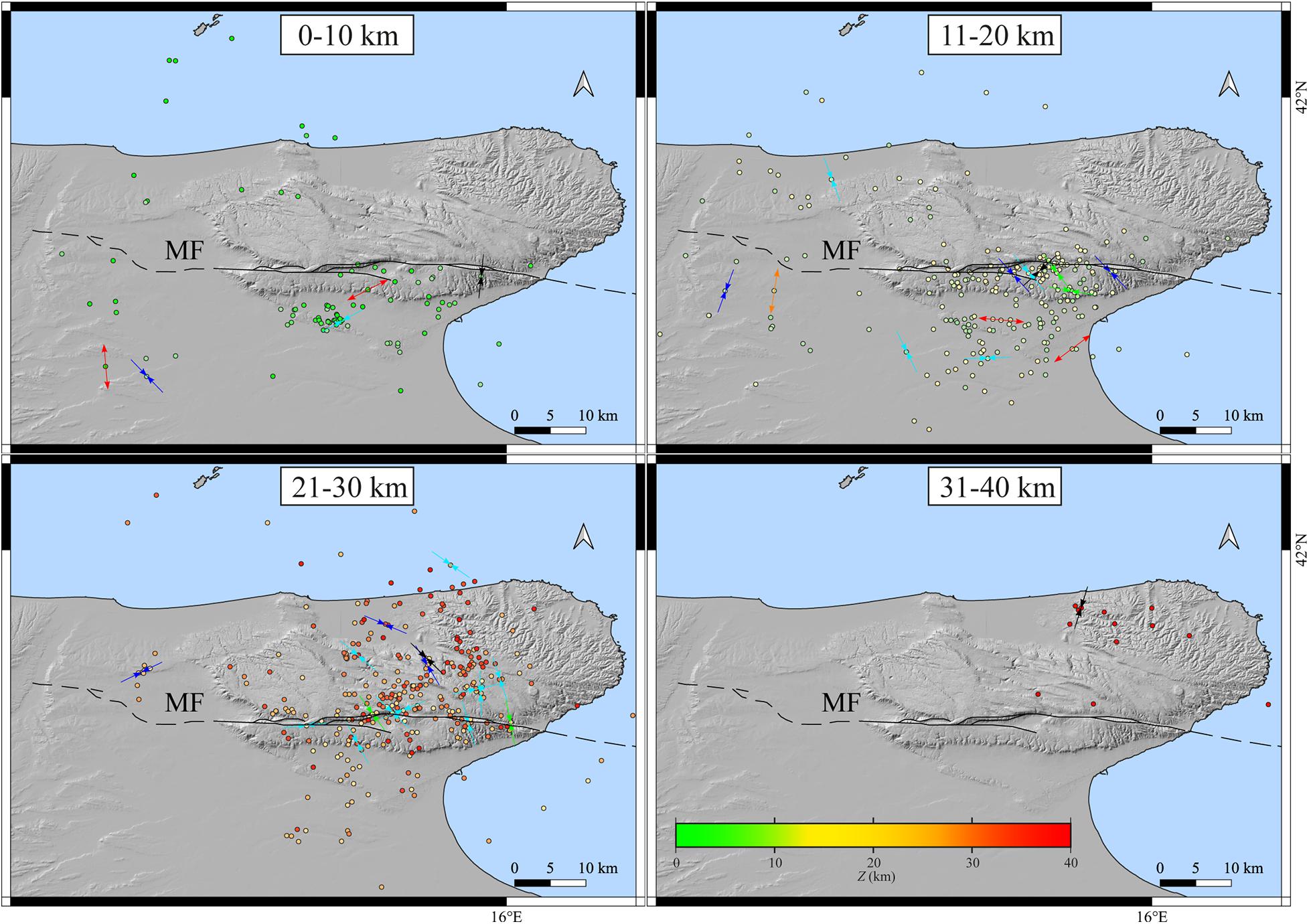
Figure 6. Geographical maps of epicentral distribution of all 635 earthquakes and 36 focal mechanisms, grouped by four depth ranges, as superimposed on each map. Epicenters are colored according to depth. described the different depth ranges. The black line is the MF System as reported by Zunino et al. (2012). Arrows represent the P-T axes with colors referring to kinematics, as shown in Figure 5.

Different kinematics can be observed at different depths (Figure 5). Normal to normal-strike events are detected at S in the GP, at shallow depths with different T-axis orientations. Twenty-two of the 36 focal mechanisms present thrust and thrust-strike kinematics, and many of them show a P-axis trending NW-SE (Figures 5B, 6). In Figure 5A, five strike-slip events, located W of the GP along the MF at Z = 20 km (except for the shallower event Ns = 18), show a right-lateral mechanism. The P-axes of these five strike-slip solutions (Figure 5B), except for the event Ns = 1, which is slightly rotated, are trending NW-SE similar to the majority of the thrust and thrust-strike P-axes. According to the results, we agree with the interpretation of the MF as a right-lateral strike-slip structure. Moreover, the inferred maximum horizontal compressive stress, S_Hmax, is SE-NW oriented (Figures 5C,D), and it is compatible with the recognized dextral strike-slip tectonics in the foreland sector of the Italian Apennines. As known from experiments, a strike-slip fault can produce a compression or an extension of the surrounding rock volumes according to its relative sense of shear; regarding the MF case, it is observed that a W-E right-lateral strike-slip structure can cause a NW-SE compression that occurs along the NE-SW-oriented strikes (Piccardi, 1998, 2005; Chilovi et al., 2000; Valensise et al., 2004; Tondi et al., 2005).

As shown in Figure 5A, nodal planes trend approximately NE-SW, with low to moderate dip angles, underlining a general compression toward NNW-SSE with NW–SE trending P-axes (Figure 5B) consistent with the data reported in the Italian Stress Map (Montone and Mariucci, 2016). Moreover, the stress inversion (Figures 5C,D) indicates a deep homogeneous compressive stress field with S_Hmax oriented NW-SE. This trend is also observed by computing the stress field in any point of the GP area. As shown in Figure 5E, the resulting S_Hmax orientation seems to be constant along the whole promontory, highlighting this NW-SE regional compression from the SW of GP to the Adriatic Sea, also according to the Italian Stress Map data (Montone and Mariucci, 2016) interpolated and shown in Carafa and Barba (2013).

Different kinematics are observed W of GP in contrast with previous studies (Carafa and Barba, 2013; Montone and Mariucci, 2016). In fact, from focal mechanism interpolation (Figure 5E), a change in the S_Hmax orientation is observed W of GP. According to Zoback (1992), this spatially concentrated variation of the maximum horizontal compressive axes may be associated to a “second-order” stress pattern due to a local perturbation of the stress field whose causes are still unknown.

The observed relation between seismicity distribution and faulting kinematics seems to suggest three hypothesis that we will investigate in the next subsections by performing vertical cross-sections: (1) the presence of a seismogenic layer trending toward NE (SW-NE cross-sections); (2) the role of the MF structure in the observed seismicity pattern (S-N cross-sections); (3) the presence of a seismogenic layer dipping toward NW (SE-NW cross-sections).

SW-NE Cross-Sections

We considered five SW-NE cross-section lines (Figure 7), orthogonal to the geomorphological evidence of compression (Bertotti et al., 1999) and parallel to the direction of surface heat flow, which decreases toward NE (Filippucci et al., 2019a) to investigate the existence of a seismogenic layer trending toward NE. Each cross-section line has a horizontal box-section with a length of about 52 and 16 km of width. Each earthquake and each focal mechanism falling into the box-section is plotted in the vertical cross-section map.

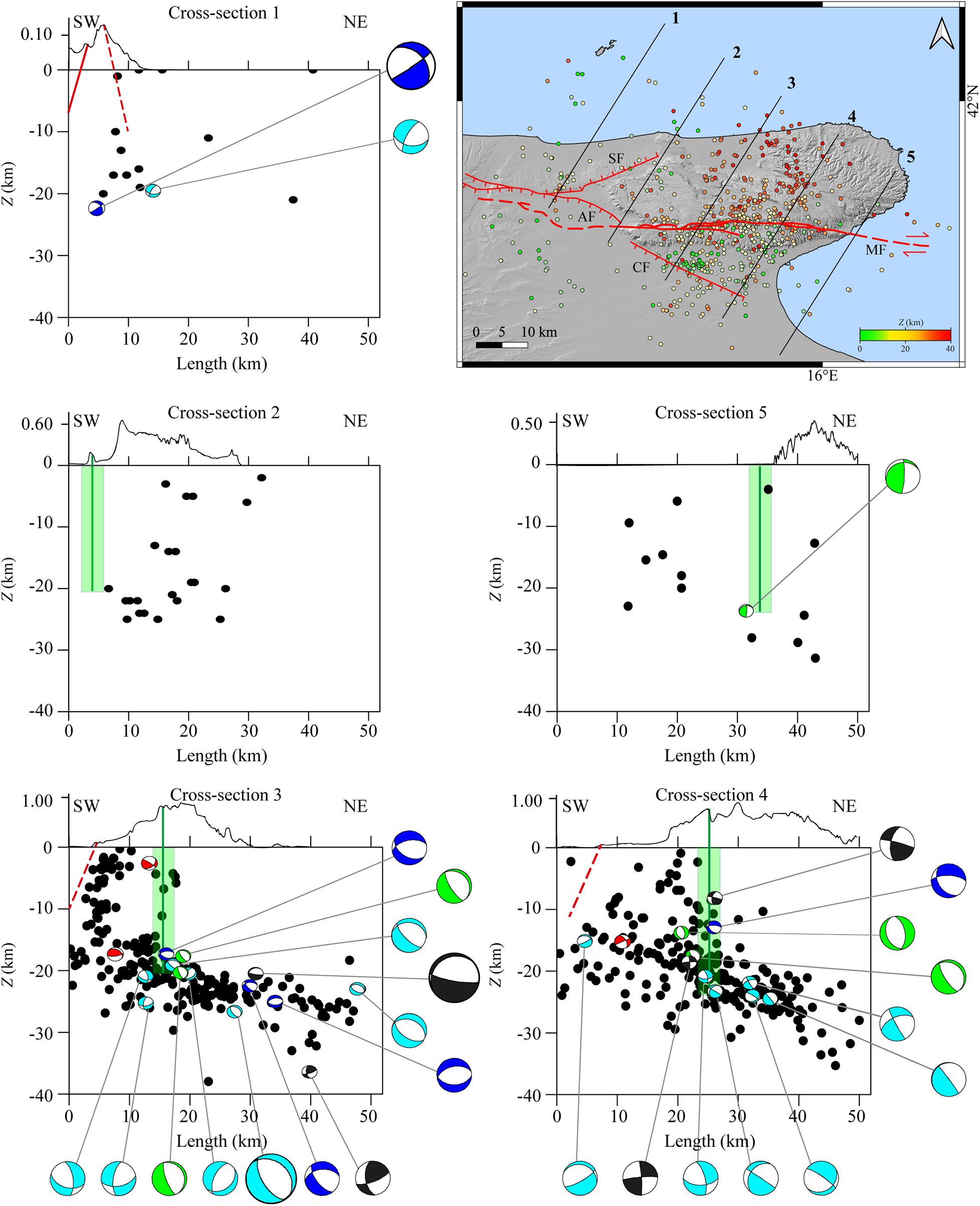
Figure 7. (Top-right) SW-NE vertical cross-sections reported as numbered black lines in the geographical map; epicenters are colored according to the color scale bar. All cross-sections have 52 km length and 8 km semi-width per side. Hypocenters are plotted as black circles in the vertical cross-section maps. Above each cross-section, the topographic profile is reported. In each cross-section map, the focal mechanisms are projected in cross-section. Beachball colors are described in Figure 5 caption. Focal mechanisms dimensions are scaled according to magnitude ranges (small for Ml < 3; big for Ml ≥ 3). Green line represents the MF trace reported in depth. The surrounding area highlighted in light green represents the rock volumes involved in the MF shear zone. Red lines are for the Apricena AF, the Candelaro CF, and the Sannicandro SF Faults, dashed lines indicate that no information is available for the fault dip and/or for the fault depth.

From cross-sections 3 and 4 (Figure 7), it is evident that a great number of events, located at Z > 15 km, occur along a slightly tilted surface that seems to dip toward the NE. It is worth to note that this deepening of seismicity probably shows the trend of the Adriatic Moho, whose depth is reported to range between 35 and 40 km (Chiarabba et al., 2005; Piana Agostinetti and Amato, 2009).

Doglioni et al. (1994) identified the high angle of the subduction plane of the Adria plate below the Apennine chain as the cause of a partial rise of the Moho and of the general uplift of the GP sector. However, the majority of focal mechanisms projected in the vertical cross-sections show nodal planes NNW-SSE oriented orthogonally to the SW-NE observed seismicity trend; therefore, these plane solutions do not seem to highlight any seismic structure trending SW-NE.

SW in the GP, normal focal mechanisms and the related shallow seismicity seem to highlight a SW dipping structure, which, however, does not seem to be related to the CF (red dashed line in Figure 7), although these events seem to indicate that some stress release involves this fractured volume of the upper crust.

It can be also observed, in the vertical cross-sections 3 and 4 (Figure 7), that in the NE of GP, seismicity is not present above 20 km and that earthquakes seem to concentrate around the area of the MF system, whose depth is estimated to range between 15 and 20 km (Piccardi, 1998; Valensise et al., 2004; DISS Working Group, 2018). For the MF shear zone, we assumed a depth of 20 km and a width of 4 km (Figure 7, green line and rectangle in vertical cross-sections) smaller than that assumed by Salvini et al. (1999) in order to reduce over-interpretation errors.

S-N Cross-Sections

We considered five SN cross-section lines oriented orthogonal to this structure (Figure 8) to investigate the role played by the MF zone in seismicity pattern and stress field. Excluding cross-sections 1 and 5 that border the MF zone, from W toward E, there is a general increase in seismicity distributed along two main probable alignments. In these three cross-sections, a lack of shallow seismicity N to the MF zone is visible (Figure 8, green line and green rectangle in the vertical cross-sections). Deep seismicity is shown in all cross-sections, but it is dominant in cross-sections 3 and 4 (Figure 8). In fact, all earthquakes appear to be located along a submerging N surface with a slightly more inclined angle moving toward E.

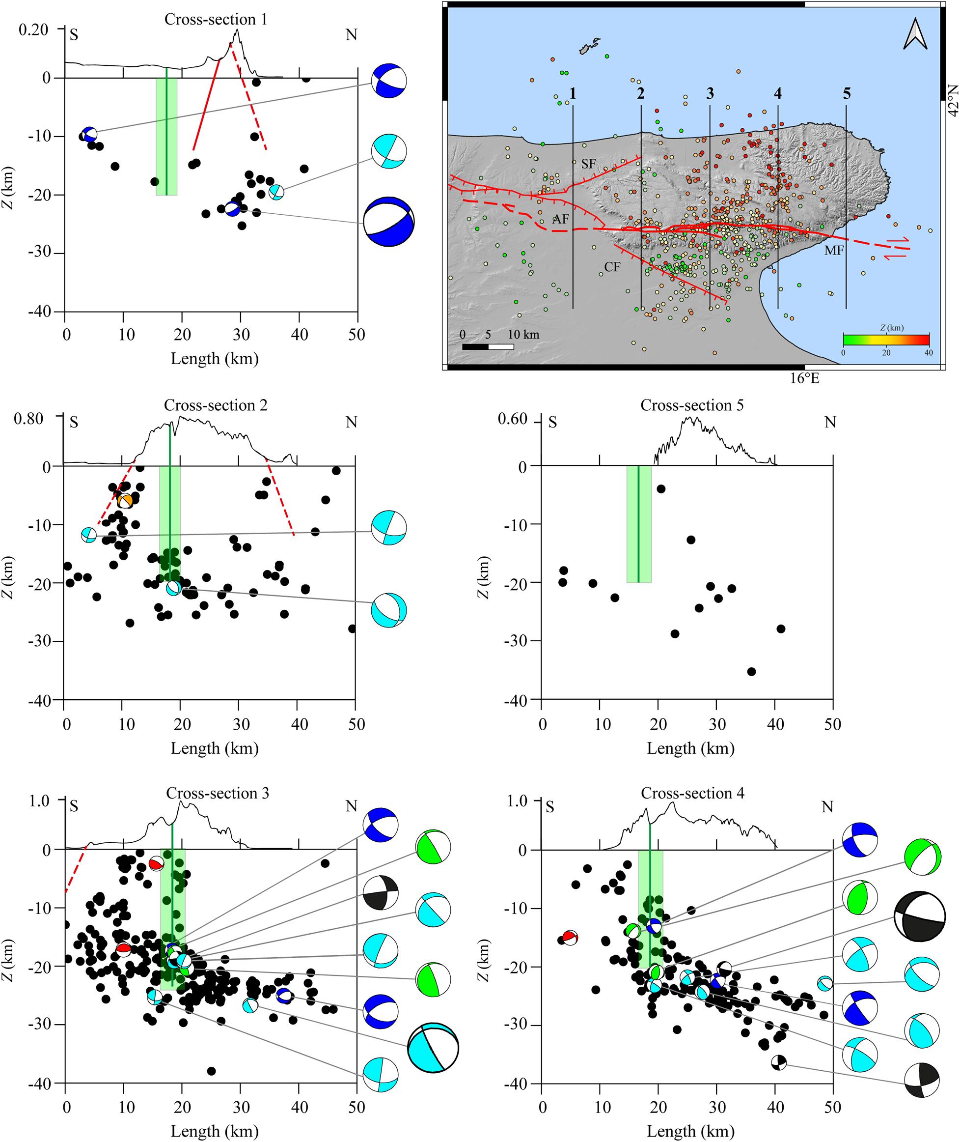
Figure 8. The same as Figure 7 for the N-S cross-sections. All cross-sections have 50 km length and 8 km semi-width per side.

The lack of shallow seismicity in the NE part of GP starting from the MF zone corroborates the hypothesis of a “natural barrier” role of the MF zone in the seismicity pattern. At the S of MF, earthquakes with normal to normal-strike faulting are observed. In cross-sections 2 and 3 (Figure 8), focal mechanisms do not allow to assert whether this seismicity belongs to CF (red dashed line in Figure 8). No events are localized along AF and SF.

Along the eastern segments of the MF at 15 < Z < 20 km (Figure 8, cross-section 3), it is possible to observe a large concentration of seismicity. This could be a hint of the presence of a splay of this deeper surface or could be caused by an area of extreme weakness that can facilitate the stress release. This second hypothesis can be confirmed by the heterogeneity of the focal mechanisms. The cross-section overlapping in Figure 9 permits to better identify the seismic horizons, the kinematic heterogeneity in the proximity of the MF structure, and the good correlation between seismicity distribution and focal mechanisms. In Figure 9A, the general seismicity trend is shown, revealing the presence of a deep surface. In fact, a great number of events appear to be aligned in depth along a slightly tilted surface. In Figure 9B, we plotted only focal mechanisms falling in proximity of the MF structure in order to highlight the kinematic heterogeneity in correspondence of the MF shear zone (Figure 9, green rectangle). The observed heterogeneity validates the idea of the existence of fractured rocks that could break with faulting kinematics, which are different from the strike-slip faulting ascribed to MF. In this frame, a focal mechanism of events located in and around the MF rectangle seems to show right-strike-slip kinematics and hints of partial reuse of the MF system in the compressive tectonic domain.

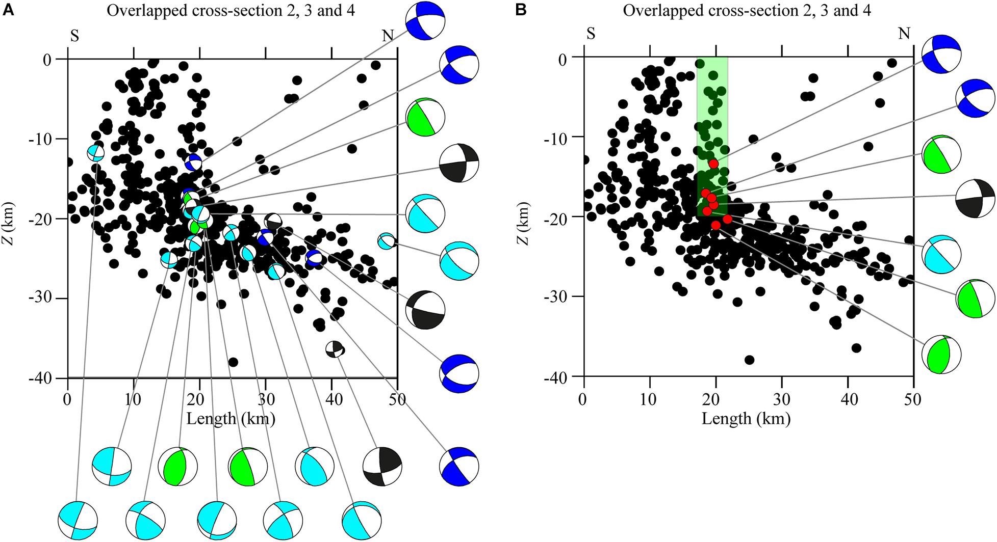
Figure 9. Overlapped cross-sections 2, 3, and 4 of Figure 8. (A) focal mechanisms are projected in cross-section. Beachball colors are as described in the Figure 5 caption. (B) A selection of focal mechanisms as described in the text with red dots indicating the hypocenters, green rectangle indicates the MF shear zone.

SE-NW Cross-Sections

We considered four cross-section lines SE-NW oriented (Figure 10), perpendicular to those of Figure 7 in order to investigate the presence of a seismogenic layer dipping toward NW. Deep events are few and quite widespread along cross-section 1 (Figure 10) so any interpretation is not possible. In cross-section 2 (Figure 10), deep seismicity seems to follow the trend previously observed in Figures 8, 9, highlighting a slope slightly dipping toward NW. Along the MF zone (Figure 10 green line and green rectangle in cross-sections), an abrupt interruption of the shallower seismicity and a greater concentration of events at Z > 15 km is observed. These features are also shown in cross-section 3 (Figure 10) where the events, close to the MF, are more concentrated at Z = 20 km. Moving from cross-sections 2–4 (Figure 10), the maximum foci depth increases, highlighting the deepening of the Moho toward the Adriatic Sea, also shown in cross-sections 3 and 4 of Figure 7. The seismicity pattern seems to confirm the presence of a low-angle surface slightly dipping N-NW that hosts this seismicity. This hypothesis seems to find an additional constraint in the plotted thrust and thrust-strike focal mechanisms (Figure 10, cross-sections 2, 3, and 4) that show one nodal plane in agreement with this hypothesized structure.

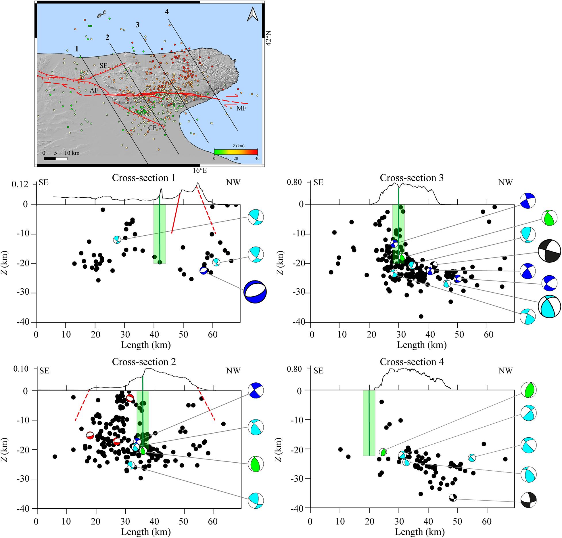
Figure 10. The same as Figure 7 for SE-NW cross-sections. All cross-sections have 69 km length and 8 km semi-width per side.

In Figure 11, the vertical cross-sections 2, 3, and 4 of Figure 10 are overlapped in order to highlight the presence of a high-angle shallower seismogenic layer and a low-angle deeper one, which trends SW-NE and slightly dips NNW. In Figure 11A, all focal mechanisms are plotted, excluding normal and normal-strike events. The seismic/aseismic transition seems to occur along a curved surface that is sketched in Figure 11B. Two interpretations can be advanced: the first one considers a low-angle deep surface (red solid line in Figure 11B), in agreement with kinematic data (red boxes, Figure 11B), with the seismicity distribution and with the general compressive/transpressive kinematic with S_Hmax NW-SE oriented; the second one considers as a seismic/aseismic transition the surface (orange dashed line in Figure 11B sketched by joining the focal mechanisms grouped in the orange boxes of, Figure 11B) around the MF shear zone (green rectangle in Figure 11B). This second interpretation agrees with a change in the dip angle of this transition surface and also agrees with the hypothesis of a local release of microearthquakes, rupturing on planes with different kinematics. The heterogeneity of the obtained focal mechanisms around the MF can be justified by the sequence of different reactivation processes over time. This observation is also confirmed by the seismicity distribution, which clusters around the MF (Figures 9, 11).

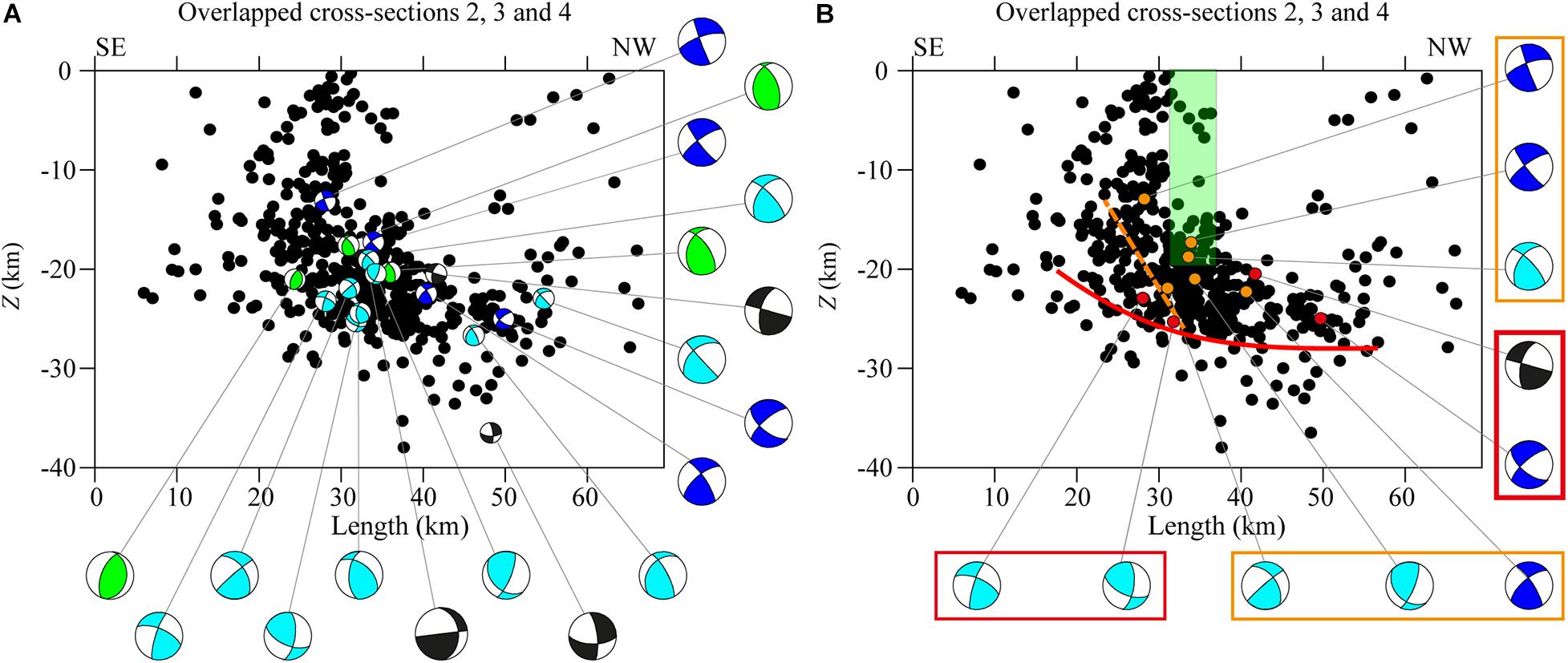
Figure 11. Overlapped vertical cross-section maps 2, 3, and 4 of Figure 10. (A) Hypocenters are reported as black circles, focal mechanisms are projected in cross-section. Beachball colors are described in Figure 5 caption. (B) Green rectangle indicates the MF system. Refer to the text for explanation of the superimposed sketched lines and of the rectangles outside the cross-section map.

Conclusion

New insights of the GP seismicity have been presented in this paper. We used the micro-earthquakes recorded from April 2013 to June 2020, with the aim of understanding a possible correlation between the low-magnitude seismicity and the known seismogenic structures. From the seismicity pattern analysis, we found out that the whole crust is seismically involved up to about Z = 40 km with an earthquake concentration at 14 < Z < 37 km. We interpret the GP seismicity as generated by a deep compressive stress regime with S_Hmax oriented NW-SE with a deep faulting NE-SW oriented. This interpretation is verified by the focal mechanisms, the stress field inversion, and stress field interpolation. Our results agree with the Italian Stress Map (Montone and Mariucci, 2016) and do not agree with the extensional present-day interpretation of Billi et al. (2007) and with the surface fault lines, which the contractional tectonic evolution of the GP is attributed to Bertotti et al. (1999).

We hypothesize the presence of a low-angle seismogenic surface trending SW-NE and dipping SE-NW. This surface could also extend in the Adriatic Sea following the same trend, according to the focal mechanisms from Pondrelli et al. (2006), to the Italian Stress Map (Montone and Mariucci, 2016) and to the interpolated stress field computed by Carafa and Barba (2013). Moreover, the seismicity localized along the Adriatic sector (Giardini et al., 2014) seems to connect the GP with the Dinaric front, spreading with a SW-NE trend along the Gargano-Dubrovnik Fault (Battaglia et al., 2004; Figure 12B). Based on GPS data (Oldow et al., 2002), Adria is supposed to be divided into two microplates, Northern and Southern Adria plates (NAd and Sad, respectively), and connected by the G Fault (Figure 12).

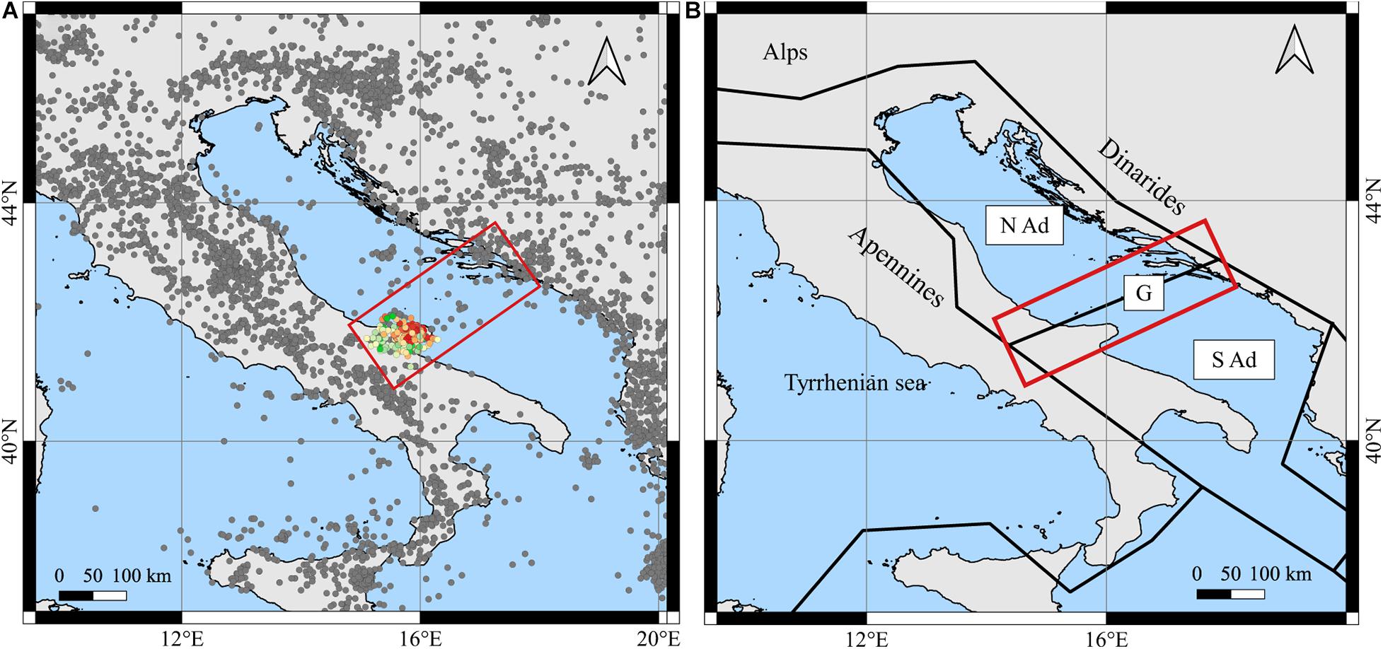
Figure 12. (A) Map of seismicity distribution in the Mediterranean area (gray dots, Giardini et al., 2014). (B) Segments (black solid lines) and modeled blocks from Battaglia et al. (2004) in a geographical map. The Gargano–Dubrovnik fault zone [G], outlined in red, was interpreted as alignment of the splits the Adria plate into two blocks: North Adria [N Ad] and South Adria [S Ad].

Regarding the role of the MF system, it cannot be stated that the whole MF is an active fault, but that some sectors of this structure are releasing the present stress field. Regarding the lack of shallow seismicity in the North-Northeast area of the GP, it can be hypothesized that deep seismicity (between 15 and 30 km) may be favored by the presence of weak preexisting fractures, lubricated by the circulation of deep fluids, as it happens in other Italian seismogenic areas (Miller et al., 2004). The presence of fluids in the upper crust was supported by geochemical analysis (Salvi et al., 1999) and resistivity imaging (Tripaldi, 2020) in proximity to CF and could explain the seismicity observed near the CF system. To disentangle this issue, which has important implications in seismic hazard, deep geophysical imaging and thermal–rheological modeling, which includes fluid convection, should be conducted.

Obviously, we cannot exclude that the lack of shallow seismicity at N will produce an earthquake energetic enough to affect the entire crustal volume, but at the same time, we cannot assert it. Some of the strongest historical earthquakes that affected this area, as the 1414 earthquake (Mw 5.8 ± 0.46), the 1646 earthquake (Mw = 6.72 ± 0.25) and also the 1889 and the 1893 events (Mw = 5.47 ± 0.12 and 5.39 ± 0.19, respectively) (data from Rovida et al., 2019), were located in this sector of GP without any information about foci depths. The September 30, 1995 earthquake (Mw = 5.15 ± 0.10) occurred at a depth of about 27 km (Del Gaudio et al., 2007), with a controversial kinematic, whether it is reverse faulting (Pondrelli et al., 2006) or E-W dextral strike-slip (Del Gaudio et al., 2007), both compatible with the stress field computed in this work.

Possible future developments of this research could be the integration of geodetic information, InSAR data (Atzori et al., 2007), and GPS data (Carafa et al., 2020), with seismic data to estimate the strain rates of the area. Moreover, new seismic data analysis and a more extended area under study around the GP could be useful to investigate how the GP is inserted in the Italian and Adriatic geodynamic context.

Data Availability Statement

Publicly available datasets were analyzed in this study. These data can be found here: Seismic waveforms for the period 2013–2018 can be found at: https://doi.org/10.17632/7b5mmdjpt3.3, while seismic waveforms for the period 2019–2020 can be found at https://www.orfeus-eu.org/data/eida/nodes/INGV/.

Author Contributions

SM organized the database and produced figures and tables. SL, MF, AF, and SM contributed to earthquake localizations. SL, MF, SM, and PP contributed to focal mechanism solutions. SM and PP performed the stress inversion. AT supervised and financed the work. MF and SM wrote the original draft. All authors contributed to conception and design of the study, manuscript revision, read, and approved the final version.

Funding

The computational work has been executed on the IT resources of the ReCaS-Bari data center, which has been made available by two projects financed by the MIUR (Italian Ministry for Education, University and Re-search) in the “PON Ricerca e Competitività 2007–2013” Program: ReCaS (Azione I– Interventi di rafforzamento strutturale, PONa3_00052, Avviso 254/Ric) and PRISMA (Asse II – Sostegno all’innovazione, PON04a2_A). This work was partially supported by Project PRIN n. 201743P29 FLUIDS (Detection and tracking of crustal fluid by multi-parametric methodologies and technologies).

Conflict of Interest

The authors declare that the research was conducted in the absence of any commercial or financial relationships that could be construed as a potential conflict of interest.

Acknowledgments

We would like to thank Federica Ferrarini and two reviewers for their suggestions, which greatly improved the manuscript. We would also like to thank Michele C. M. Carafa for stimulating discussion and for assistance using the software SHINE. Figures were obtained by employing the GMT freeware package by Wessel and Smith (1998) and by employing the QGIS free software, v 3.8 (www.qgis.org).

Supplementary Material

The Supplementary Material for this article can be found online at: https://www.frontiersin.org/articles/10.3389/feart.2021.589332/full#supplementary-material

Supplementary Figure 1 | Focal mechanism solutions obtained, respectively with the average, the minimum and the maximum velocity model. Ns is the identification number for each solution. Events with Ns 1–6 are shown.

Supplementary Figure 2 | Same as Supplementary Figure 1. Events with Ns 7–12 are shown.

Supplementary Figure 3 | Same as Supplementary Figure 1. Events with Ns 13–18 are shown.

Supplementary Figure 4 | Same as Supplementary Figure 1. Events with Ns 19–24 are shown.

Supplementary Figure 5 | Same as Supplementary Figure 1. Events with Ns 25–30 are shown.

Supplementary Figure 6 | Same as SupplementaryFigure 1. Events with Ns 31–36 are shown.

Supplementary Table 1 | List of localizations of the 635 earthquakes. ID: event identification number; Origin Time; Lon (decimal degrees), Lat (decimal degrees), Z (km): localization parameters; Ml: magnitude (see text for explanation); Ph: Number of P-wave and S-wave phases; θ: azimuthal gap; d_min: minimum distance; RMS: root mean square (s); ERH: horizontal error (km); ERZ: vertical error (km); QM: localization quality as output of Hypo71; S: dimensionless parameter (see the text for explanation).

Supplementary Table 2 | Localizations obtained with error propagation. Ns: focal mechanism identification number; Origin time: event origin time; Lon (decimal degrees), Lat (decimal degrees) and Z (km) computed with the average (AVG) velocity model, the minimum (MIN) and maximum (MAX), respectively (see the text for explanation); ED (m): epicentral distance; MIN difference between the epicenter computed with the average and minimum model; MAX difference between the epicenter computed with the maximum and the average model. VD (m): vertical distance: MIN difference between hypocenters computed with the average and minimum model; MAX difference between the hypocenters computed with the maximum and average model.

References

Anderson, H. A., and Jackson, J. A. (1987). Active tectonics of the Adriatic region. Geophys. J. R. Astron. Soc. 91, 937–983. doi: 10.1111/j.1365-246X.1987.tb01675.x
Argnani, A., Favali, P., Frugoni, F., Gasperini, M., Ligi, M., Marani, M., et al. (1993). Foreland deformational pattern in the southern Adriatic Sea. Ann. Geofis. 36, 229–247. doi: 10.4401/ag-4279
Argnani, A., Rovere, M., and Bonazzi, C. (2009). Tectonics of the Mattinata fault, offshore south Gargano (southern Adriatic Sea, Italy): implications for active deformation and seismotectonics in the foreland of the southern Apennines. Geol. Soc. Am. Bull. 121, 1421–1440. doi: 10.1130/B26326.1
Atzori, S., Hunstad, I., Tolomei, C., Salvi, S., Ferretti, A., and Cespa, S. (2007). Interseismic Strain Accumulation in the Gargano Promontory, Central Italy. Geophysical Research Abstracts 9, Abstract EGU 2007-A-07651. Munich: European Geosciences Union.
Battaglia, M., Murray, M. H., Serpelloni, E., and Bürgmann, R. (2004). The Adriatic region: an independent microplate within the Africa−Eurasia collision zone. Geophys. Res. Lett. 31:L09605. doi: 10.1029/2004GL019723
Bertotti, G., Casolari, E., and Picotti, V. (1999). The Gargano promontory: a neogene contractional belt within the Adriatic plate. Terra Nova 11, 168–173. doi: 10.1046/j.1365-3121.1999.00243.x
Billi, A., Gambini, R., Nicolai, C., and Storti, F. (2007). Neogene-Quaternary intraforeland transpression along a Mesozoic platform-basin margin: the Gargano fault system, Adria, Italy. Geosphere 3, 1–15. doi: 10.1130/GES00057.1
Bosellini, A., and Morsilli, M. (2001). Il Promontorio del Gargano cenni di Geologia e Itinerari Geologici: Claudio Grenzi Editore. Sant’Angelo: Parco Nazionale del Gargano, 1–48.
Brankman, C., and Aydin, A. (2004). Uplift and contractional deformation along a segmented strike-slip fault system: the Gargano Promontory, southern Italy. J. Struct. Geol. 26, 807–824. doi: 10.1016/j.jsg.2003.08.018
Carafa, M. M. C., and Barba, S. (2013). The stress field in Europe: optimal orientations with confidence limits. Geophys. J. Int. 193, 531–548. doi: 10.1093/gji/ggt024
Carafa, M. M. C., Barba, S., and Bird, P. (2015b). Neotectonics and long−term seismicity in Europe and the Mediterranean region. J. Geophys. Res. Solid Earth 120, 5311–5342. doi: 10.1002/2014JB011751
Carafa, M. M. C., Galvani, A., Di Naccio, D., Kastelic, V., Di Lorenzo, C., Miccolis, S., et al. (2020). Partitioning the ongoing extension of the central Apennines (Italy): fault slip rates and bulk deformation rates from geodetic and stress data. J. Geophys.Res. Solid Earth 125:e2019JB018956. doi: 10.1029/2019JB018956
Carafa, M. M. C., Tarabusi, G., and Kastelic, V. (2015a). SHINE: web application for determining the horizontal stress orientation. Comput. Geosci. 74, 39–49. doi: 10.1016/j.cageo.2014.10.001
Chiarabba, C., Jovane, L., and DiStefano, R. (2005). A new view of Italian seismicity using 20 years of instrumental recordings. Tectonophysics 395, 251–268. doi: 10.1016/j.tecto.2004.09.013
Chilovi, C., De Feyter, A. J., and Pompucci, A. (2000). Wrench zone reactivation in the Adriatic Block: the example of the Mattinata Fault System (SE Italy). Boll. Soc. Geol. Ital. 119, 3–8.
Cotecchia, V. (2014). Le acque sotterranee e l’intrusione marina in Puglia: dalla ricerca all’emergenza nella salvaguardia della risorsa. Mem. Descr. Carta Geol. XCII, 15–660.
de Lorenzo, S., Michele, M., Emolo, A., and Tallarico, A. (2017). A 1D P-wave velocity model of the Gargano promontory (southeastern Italy). J. Seismol. 21, 909–919. doi: 10.1007/s10950-017-9643-7
Del Gaudio, V., Pierri, P., Frepoli, A., Calcagnile, G., Venisti, N., and Cimini, G. (2007). A critical revision of the seismicity of northern Apulia (Adriatic microplate – Southern Italy) and implications for the identification of seismogenic structures. Tectonophysics 436, 9–35. doi: 10.1016/j.tecto.2007.02.013
Di Bucci, D., and Angeloni, P. (2013). “Adria seismicity and seismotectonics: review and critical discussion. Special issue,” in The Geology of the Periadriatic Basin and the Adriatic Sea, Vol. 42, eds S. Bigi, C. D’Ambrogi, and E. Carminati (Cham: Springer), 182–190. doi: 10.1016/j.marpetgeo.2012.09.005
DISS Working Group (2018). Database of Individual Seismogenic Sources (DISS), Version 3.2.1: A Compilation of Potential Sources for Earthquakes Larger than M 5.5 in Italy and Surrounding Areas. doi: 10.6092/INGV.IT-DISS3.2.1
Doglioni, C., Mongelli, F., and Pieri, P. (1994). The Puglia uplift (SE Italy): an anomaly in the foreland of the Apenninic subduction due to buckling of a thick continental lithosphere. Tectonics 13, 1309–1321. doi: 10.1029/94TC01501
Favali, P., Mele, G., and Mattietti, G. (1990). Contribution to the study of the Apulian microplate geodynamics. Mem. Soc. Geol. Ital. 44, 71–80.
Filippucci, M., Del Pezzo, E., de Lorenzo, S., and Tallarico, A. (2019b). 2D kernel-based imaging of coda-Q space variations in the Gargano Promontory (Southern Italy). Phys. Earth Planet. Int. 297:106313. doi: 10.1016/j.pepi.2019.106313
Filippucci, M., Miccolis, S., Castagnozzi, A., Cecere, G., de Lorenzo, S., Donvito, G., et al. (2021a). Seismicity of the Gargano Promontory (Southern Italy) after 7 years of local seismic network operation: data release of waveform from 2013 to 2018. Data Brief. 35:106783. doi: 10.1016/j.dib.2021.106783
Filippucci, M., Miccolis, S., Castagnozzi, A., Cecere, G., de Lorenzo, S., Donvito, G., et al. (2021b). Gargano Promontory (Italy) microseismicity (2013-2018): waveform data and earthquake catalogue. Mendeley Data doi: 10.17632/7b5mmdjpt3.3 [Epub ahead of print].
Filippucci, M., Pierri, P., de Lorenzo, S., and Tallarico, A. (2020). “The stress field in the Northern Apulia (Southern Italy), as deduced from microearthquake focal mechanisms: new insight from local seismic monitoring,” in Computational Science and Its Applications – ICCSA 2020. Lecture Notes in Computer Science, Vol. 12255, eds O. Gervasi, B. Murgante, S. Misra, C. Garau, I. Blečić, D. Taniar, et al. (Cham: Springer), 914–927. doi: 10.1007/978-3-030-58820-5_66
Filippucci, M., Tallarico, A., Dragoni, M., and de Lorenzo, S. (2019a). Relationship between depth of seismicity and heat flow: the case of the Gargano area (Italy). Pure Appl. Geophys. 176, 2383–2394. doi: 10.1007/s00024-019-02107-5
Frepoli, A., Cimini, G. B., De Gori, P., De Luca, G., Marchetti, A., Monna, S., et al. (2017). Seismic sequences and swarms in the Latium-Abruzzo-Molise Apennines (Central Italy): new observations and analysis from a dense monitoring of the recent activity. Tectonophysics 712-713, 312–329. doi: 10.1016/j.tecto.2017.05.026
Frepoli, A., Maggi, C., Cimini, G. B., Marchetti, A., and Chiappini, M. (2011). Seismotectonic of Southern Apennines from recent passive seismic experiments. J. Geodyn. 51, 110–124. doi: 10.1016/j.jog.2010.02.007
Funiciello, R., Montone, P., Salvini, F., and Tozzi, M. (1988). Caratteri strutturali del Promontorio del Gargano. Mem. Soc. Geol. Ital. 41, 1235–1243.
Gephart, J. W. (1990). FMSI: a FORTRAN program for inverting fault/slickenside and earthquake focal mechanism data to obtain the regional stress tensor. Comput. Geosci. 16, 953–989. doi: 10.1016/0098-3004(90)90105-3
Gephart, J. W., and Forsyth, D. W. (1984). An improved method for determining the regional stress tensor using earthquake focal mechanism data: application to the San Fernando Earthquake Sequence. J. Geophys. Res. 89, 9305–9320. doi: 10.1029/JB089iB11p09305
Giardini, D., Woessner, J., and Danciu, L. (2014). Mapping europe’s seismic hazard. EOS 95, 261–262.
Hardebeck, J. L., and Shearer, P. M. (2002). A new method for determining first-motion focal mechanisms. Bull. Seismol. Soc. Am. 92, 2264–2276. doi: 10.1785/0120010200
Heidbach, O., Rajabi, M., Reiter, K., and Ziegler, M. (2016). World Stress Map 2016. Potsdam: GFZ Data Services.
Helmholtz Centre Potsdam GFZ German Research Centre for Geosciences and gempa GmbH (2008). The SeisComP Seismological Software Package. Potsdam: GFZ Data Services, doi: 10.5880/GFZ.2.4.2020.003
Lee, W. H. K., and Lahr, J. C. (1972). HYPO71: A Computer Program for Determining Hypocenter, Magnitude, and first Motion Pattern of Local Earthquakes. Open-File Report 72-224. Reston, VA: US Geological Survey, doi: 10.3133/ofr72224
Lu, Z., Wyss, M., and Pulpan, H. (1997). Details of stress directions in the Alaska subduction zone from fault plane solutions. J. Geophys. Res. Solid Earth 102, 5385–5402.
Mantovani, E., Babbucci, D., Viti, M., Albarello, D., Mugnaioli, E., Cenni, N., et al. (2006). “Post-Late Miocene kinematics of the Adria microplate: inferences from geological, geophysical and geodetic data,” in The Adria Microplate: GPS Geodesy, Tectonics and Hazards. Nato Science Series: IV: Earth and Environmental Sciences, Vol. 61, eds N. Pinter, G. Gyula, J. Weber, S. Stein, and D. Medak (Dordrecht: Springer), 51–69. doi: 10.1007/1-4020-4235-3_04
McKenzie, D. (1972). Active tectonics of the Mediterranean region. R. Astronomic. Soc. Geophys. J. 30, 109–185.
Michele, M. (2016). Three-Dimensional Seismic Imaging of P and S Waves for the Gargano Promontory (Southern East Italy). Ph. D. Thesis. Bari: University of Bari.
Miller, S. A., Collettini, C., Chiaraluce, L., Cocco, M., Barchi, M., and Boris, J. P. K. (2004). Aftershocks driven by a high-pressure CO2 source at depth. Lett. Nat. 427, 724–727. doi: 10.1038/nature02251
Mongelli, F., and Ricchetti, G. (1970). Heat flow along the candelaro fault – Gargano Headland (Italy). Geothermics 2, 450–458.
Montone, P., and Mariucci, M. T. (2016). The new release of the Italian contemporary stress map. Geophys. J. Int. 205, 1525–1531. doi: 10.1093/gji/ggw100
Oldow, J. S., Ferranti, L., Lewis, D. S., Campbell, J. K., D’Argenio, B., Catalano, R., et al. (2002). Active fragmentation of Adria, the north Africa promontory, central Mediterranean orogen. Geology 30, 779–782.
Patacca, E., and Scandone, P. (2004). The 1627 Gargano earthquake (Southern Italy): Identification and characterization of the causative fault. J. Seismol. 8, 259–273.
Piana Agostinetti, N., and Amato, A. (2009). Moho depth and Vp/Vs ratio in peninsular Italy from teleseismic receiver functions. J. Geophys. Res. 114:B06303. doi: 10.1029/2008JB005899
Piccardi, L. (1998). Cinematica attuale, comportamento sismico e sismologia storica della faglia di Monte Sant’Angelo (Gargano, Italia): la possibile rottura superficiale del “leggendario” terremoto del 493 d.C. Geogr. Fis. Dinam. Quat. 21, 155–166.
Piccardi, L. (2005). Paleoseismic evidence of legendary earthquakes: the apparition of Archangel Michael at Monte Sant’Angelo (Italy). Tectonophysics 408, 113–128. doi: 10.1016/j.tecto.2005.05.041
Pondrelli, S., Salimbeni, S., Ekström, G., Morelli, A., Gasperini, P., and Vannucci, G. (2006). The Italian CMT dataset from 1977 to the present. Phys. Earth Planet. Inter. 159, 286–303. doi: 10.1016/j.pepi.2006.07.008
Reasenberg, P., and Oppenheimer, D. (1985). FPFIT, FPPLOT and FPPAGE: Fortran Computer Programs for Calculating and Displaying Earthquake Fault-Plane Solutions. USGS Open-File Report. 85-739. Reston, VA: U.S. Geological Survey. doi: 10.3133/ofr85739
Rovida, A., Locati, M., Camassi, R., Lolli, B., and Gasperini, P. (2019). Catalogo Parametrico dei Terremoti Italiani (CPTI15), versione 2.0. Rome: Istituto Nazionale di Geofisica e Vulcanologia, doi: 10.13127/CPTI/CPTI15.2
Salvi, S., Quattrocchi, F., Brunori, C. A., Doumaz, F., Angelone, M., Billi, A., et al. (1999). A multidisciplinary approach to earthquake research: implementation of a geochemical geographic information system for the Gargano Site, Southern Italy. Nat. Hazards 20, 255–278.
Salvini, F., Billi, A., and Wise, D. U. (1999). Strike-slip fault-propagation cleavage in carbonate rocks: the Mattinata Fault Zone, Southern Apennines, Italy. J. Struct. Geol. 21, 1731–1749. doi: 10.1016/S0191-8141(99)00120-0
Scisciani, V., and Calamita, F. (2009). Active intraplate deformation within Adria: examples from the Adriatic region. Tectonophysics 476, 57–72. doi: 10.1016/j.tecto.2008.10.030
Snoke, J. A. (2017). FOCMEC: FOCal MEChanism Determinations. Available online at: http://www.iris.edu/pub/programs/focmec/ (accessed February, 2020).
Snoke, J. A., Munsey, J. W., Teague, A. C., and Bollinger, G. A. (1984). A program for focal mechanism determination by combined use of polarity and SV-P amplitude ratio data. Earthquake Notes 55, 1–15.
Tallarico, A. (2013). OTRIONS Project. Available online at: http://www.otrions.uniba.it/ (accessed May 2018)
Tondi, E., Piccardi, L., Cacon, S., Kontny, B., and Cello, G. (2005). Structural and time constraints for dextral shear along the seismogenic Mattinata fault (Gargano, Southern Italy). J. Geodyn. 40, 134–152.
Tripaldi, S. (2020). Electrical signatures of a permeable zone in carbonates hosting local geothermal manifestations: Insights for the deep fluid flow in the gargano area (South-eastern Italy). B. Geofis. Teor. Appl. 61, 219–232. doi: 10.4430/bgta0312
Valensise, G., Pantosti, D., and Basili, R. (2004). Seismology and tectonic setting of the Molise earthquake sequence of October 31–November 1, 2002. Earthquake Spectra 20, 23–37.
Waldhauser, F., and Ellsworth, W. L. (2000). A double-difference earthquake location algorithm: Method application to the northern Hayward fault. Bull. Seismol. Soc. Am. 90, 1353–1368. doi: 10.1785/0120000006
Wessel, P., and Smith, W. H. F. (1998). New, improved version of generic mapping tools released. Eos Trans. Am. Geophys. 79:579. doi: 10.1029/98EO00426
Zoback, M. L. (1992). First and second order patterns of stress in the lithosphere: the world stress map project. J. Geophys. Res. 97, 11703–11728. doi: 10.1029/92JB00132
Keywords: gargano promontory, OTRIONS local seismic network, focal mechanisms, stress field, microseismicity, mattinata fault, gargano-dubrovnik lineament
Citation: Miccolis S, Filippucci M, de Lorenzo S, Frepoli A, Pierri P and Tallarico A (2021) Seismogenic Structure Orientation and Stress Field of the Gargano Promontory (Southern Italy) From Microseismicity Analysis. Front. Earth Sci. 9:589332. doi: 10.3389/feart.2021.589332
Received: 30 July 2020; Accepted: 01 March 2021;
Published: 26 April 2021.
Edited by:
Federica Ferrarini, G. d’Annunzio University of Chieti and Pescara, ItalyReviewed by:
Yohei Yukutake, Hot Spring Geology Research Institute, JapanEzgi Karasozen, University of Alaska Fairbanks, United States
Copyright © 2021 Miccolis, Filippucci, de Lorenzo, Frepoli, Pierri and Tallarico. This is an open-access article distributed under the terms of the Creative Commons Attribution License (CC BY). The use, distribution or reproduction in other forums is permitted, provided the original author(s) and the copyright owner(s) are credited and that the original publication in this journal is cited, in accordance with accepted academic practice. No use, distribution or reproduction is permitted which does not comply with these terms.
*Correspondence: Simona Miccolis, simona.miccolis@uniba.it; Marilena Filippucci, marilena.filippucci@uniba.it