
Abstract
We propose a one-parameter family of random walk processes on hypergraphs, where a parameter biases the dynamics of the walker towards hyperedges of low or high cardinality. We show that for each value of the parameter, the resulting process defines its own hypergraph projection on a weighted network. We then explore the differences between them by considering the community structure associated to each random walk process. To do so, we adapt the Markov stability framework to hypergraphs and test it on artificial and real-world hypergraphs.
Export citation and abstract BibTeX RIS

Original content from this work may be used under the terms of the Creative Commons Attribution 4.0 licence. Any further distribution of this work must maintain attribution to the author(s) and the title of the work, journal citation and DOI.
1. Introduction
In the last two decades, networks have emerged as a powerful framework to model and study complex systems [1, 2], providing a rich set of tools and methods that can be used independently of the nature of their constituting components [3–5]. At the core of network science, there is the interplay between structure and dynamics [6–8], as the topology imposes constraints of how dynamical processes propagate between nodes and, reversely, dynamical processes are at the core of several algorithms to extract information from the underlying structure [9]. An important context where this interplay is essential is the modular, or community, structure of networks. On the one hand, several works have shown that the presence of communities slows down diffusive processes on networks, in particular random walk processes [10]. Here, communities are understood as groups of densely connected nodes, leading to the presence of bottlenecks between communities. Important concepts include the Cheeger inequality, providing relations between the mixing time, e.g. time for a random walk process to relax to stationarity, and the notion of conductance, quantifying the bottlenecks in networks. On the other hand, random walk processes are at the heart of several algorithms to extract communities in networks. Community detection [11] is a central element in the toolkit of network science, allowing to produce coarse-grained representation of large-scale networks [12, 13] and thus to identify groups of nodes whose behaviour is relevant for the process under study. Methods based on random walks include the Map equation [14] and Markov stability [15, 16], exploiting the fact that good communities tend to capture random walkers for long times before they can escape them.
Networks make assumptions about the structure of interacting systems, often implicitly, and recent research has questioned the relevance of these assumptions in real-world data, leading to the concept of higher-order networks [17, 18]. In networks, for instance, the building blocks for interactions are pairwise interactions, and the whole network is formed by combining such pairwise interactions. In contrast, many interacting systems are made of interactions that involve more than two nodes and can not be decomposed further, i.e. they act as a whole. A canonical example is collaboration networks, where groups of authors interact to produce research papers [19, 20]: the emerging results are a product of the group rather than reflecting pairwise interexchanges. More generally, systems characterised by multibody interactions abound in a variety of scientific domains, from functional brain networks [21, 22] to protein interaction networks [23] and ecology [24].
The inadequacy of standard networks to model multibody interactions motivates the development of appropriate higher-order models, often enriching and generalising the standard network paradigm. The two most popular approaches are simplicial complexes [25–27] and hypergraphs [28–30]. Simplicial complexes are a model from topological data analysis, whose aim is to characterise the shape of data, in terms of the presence of holes between the points, and have been proposed as generalisations of networks with applications in epidemic spreading [31, 32] and synchronisation [33, 34]. The focus of this paper is on hypergraphs, a domain that has a long tradition in graph theory [28] but whose impact on dynamics has only been considered more recently. Recent works include applications to social contagion model [35, 36], the modelling of random walks [20], the study of synchronisation [37–39], diffusion [36], non-linear consensus [40] and the emergence of Turing patterns [39]. Hypergraphs constitute a powerful and flexible paradigm, as they encode interactions by hyperedges, defined as groups of arbitrary size between nodes. In situations when all the hyperedges have size 2, hypergraphs reduce to standard networks. Hypergraphs have several advantages, as they allow to efficiently handle very large hyperedges and, even more importantly, a heterogeneous distribution of hyperedges' sizes. Moreover, the information on the high-order structure of the embedding support are stored in a matrix whose dimension depends only on the number of nodes [20, 36] thus avoiding the use of tensors.
The main purpose of this paper is to explore the interplay between dynamics and structure in hypergraphs. More specifically, we will generalise the notion of Markov stability. As we will discover, different types of random walk processes, and their associated Laplacian, can be defined on hypergraphs, each leading to different quality functions and different partitions into communities. This flexibility originates from the fact that hyperedges are characterised by a feature, their size, and that a choice has to be made to model how this feature affects the diffusion. Classical studies in graph theory often assume that the hypergraphs are uniform, that is the hyperedges all have the same size [41, 42]. The first random walk Laplacian defined for general hypergraphs can probably be traced back to the seminal paper of Zhou et al [43], where each hyperedge is endowed with an arbitrary weight, acting as a bias to the walkers dynamics. While this weight is often considered to be a free parameter that can be chosen a priori, it may naturally emerge in certain models, such as in [20] where the transition rates of the process are linearly biased by the size of the hyperedges, i.e. a walker follows a hyperedge proportionally to its size. In general, different choices for this weight, and the resulting biases on the random walk trajectories, lead to different transition matrices. Our main result is to investigate and to characterise how these differences translate into different communities in hypergraphs.
This paper is organised as follows. In section 2, we define random walks on hypergraphs and introduce a one-parameter family of processes, extending previous models. In section 3, we generalise the concept of Markov stability to hypergraphs and, in section 4, we explore the impact of the parameter of the random walk process on the uncovered communities, looking at both artificial and real-world networks. Finally, in section 5, we conclude and discuss the implications of our work.
2. Hypergraphs and random walks
Let us consider an hypergraph  , where V = {v1, ..., vn
} denotes the set of n nodes and E = {E1, ..., Em
} the set of m hyperedges, that is for all α = 1, ..., m: Eα
⊂ V, i.e. an unordered collection of vertices. Note that if Eα
= {u, v}, i.e. |Eα
| = 2, then the hyperedge is actually a 'standard' edge denoting a binary interaction among u and v. If all hyperedges have size 2, the hypergraph is thus a network. The hypergraph can be encoded by its incidence matrix
eiα
, where we adopt the convention of using roman indexes for nodes and Greek ones for hyperedges
, where V = {v1, ..., vn
} denotes the set of n nodes and E = {E1, ..., Em
} the set of m hyperedges, that is for all α = 1, ..., m: Eα
⊂ V, i.e. an unordered collection of vertices. Note that if Eα
= {u, v}, i.e. |Eα
| = 2, then the hyperedge is actually a 'standard' edge denoting a binary interaction among u and v. If all hyperedges have size 2, the hypergraph is thus a network. The hypergraph can be encoded by its incidence matrix
eiα
, where we adopt the convention of using roman indexes for nodes and Greek ones for hyperedges

A standard procedure to construct the n × n adjacency matrix of the hypergraph is A = eeT, whose entry Aij represents the number of hyperedges containing both nodes i and j. Note that it is often customary to set to zero the diagonal elements of the adjacency matrix. Let us also define the m × m hyperedges matrix B = eT e, whose entry Bαβ counts the number of nodes in Eα ∩ Eβ . B can be seen as the (weighted) adjacency matrix of the dual hypergraph, i.e. where hyperedges of the original hypergraph become nodes of the new structure and two nodes are connected by a weighted link counting how many nodes (in the original hypergraph) are shared by the two hyperedges, namely Bαβ . Note that a similar construction has been proposed in [44] to extract a n-clique graph from a network, namely a network whose nodes are the n-clique of the original one and whose nodes are connected if the n-clique share at least one node (in the original network). The main difference in the present case is that hyperedges can have an heterogeneous size distribution and thus provide a more flexible framework.
We can define a random walk process on a hypergraph as follows. The agents are located on the nodes and hop between nodes at discrete times. In a general setting, the walkers may give more or less importance to hyperedges depending on their size, a choice that may then bias their moves [20]. This process is captured by the weighted adjacency matrix

where σ is a real parameter whose role will be discussed in the following; note that Bαα − 1 denotes the number of nodes in the hyperedge Eα available to the walker, i.e. discarding the node where she is sitting initially. It is worth emphasising that in principle we could have used a generic monotone function f of the hyperedge size, in defining the above quantities. For illustrative purposes we have here chosen to limit the analysis to the relevant, although particular, setting of a power law bias. The transition probabilities of the examined process are then obtained by normalising the columns of the weighted adjacency matrix

Note that a 'lazy' process could have been defined by assuming that walkers are able to stay put on a node in one step, for instance by taking  .
.
This general definition covers several existing models of random walks on hypergraphs. For σ = 1, we get the random walk defined in [20] while for σ = −1 we obtain the one introduced by Zhou et al [43], as

and

where we used the fact ∑ℓ≠i eℓα equals the number of nodes in Eα without node i, that is (Bαα − 1), which thus simplifies with the denominator. The last equality defines ki to be number of hyperedges incident to node i, a quantity that is simply the node degree in the case of networks. In conclusion,

has the following interpretation: the walker sitting on node i choses uniformly at random one hyperedge among the incident ones, i.e. with probability 1/ki , and then it selects a node belonging to the latter, again uniformly at random, i.e. with probability 1/(Bαα − 1).
The case σ = 0 returns a random walk on the so called clique reduced multigraph. The latter is a multigraph where each pair of nodes is connected by a number of edges equal to the number of hyperedges containing that pair in the hypergraph (see top left panel of figure 1). In that case, the transition matrix simplifies into

where we used the definition of the hyperadjacency matrix Aij = ∑α eiα ejα . Let us observe that the clique reduced multigraph is different from the projected network obtained by associating to each hyperedge a clique of the same size; the projected network can be interpreted as the unweighted (binarised) version of the clique reduced multigraph (see bottom left panel of figure 1).

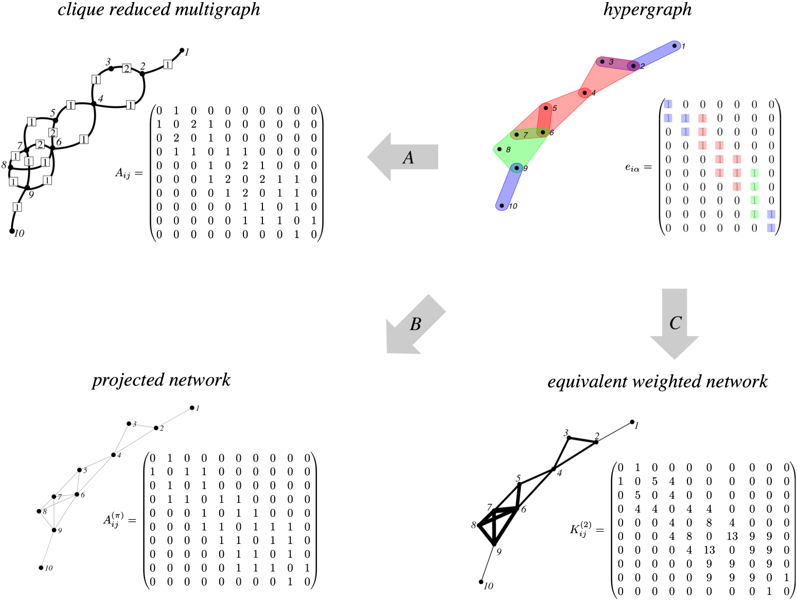
Figure 1. Hypergraph and their projection. The top right panel shows a hypergraph, where hyperedges of different sizes are shown in different colours, the three two-hyperedges are coloured in blue ({1, 2}, {2, 3} and {9, 10}), the three three-hyperedges are coloured in red ({2, 3, 4}, {4, 5, 6} and {5, 6, 7}) and the four-hyperedge in green ({6, 7, 8, 9}). Hyperedges do overlap and this 'creates' new colours that are not associated to new hyperedges. Its structure is entirely encoded in the incidence matrix eiα where, for ease of visualisation, we use the same colour code. Different projections can be constructed from the same hypergraph, each leading to a different weighted graph. In the clique reduced multigraph (top left panel), links between two nodes carry a weight proportional to the number of hyperedges including these two nodes. Alternatively, the so-called projected network is a binarised version of the clique reduction multigraph, so that a link exists between two nodes if they belong to at least one hyperedge. Finally, the family of projections K(σ) defined in this paper, illustrated for the case σ = 2 at the bottom right, gives more or less weight to edges depending on the size of the hyperedges from which they are built.
Download figure:
Standard image High-resolution imageFrom the definitions (2) and (3), it is clear that hyperedges with larger sizes will dominate and, thus, set the fate of the random process for large values of σ. When σ is very negative, in contrast, hyperedges with a small size will drive the random walk process. As such, σ can be pictured as a size bias parameter which dictates the importance of hyperedges depending on their size.
Given the transition probability (3), a continuous-time random walk can be defined by

where pi
(t) is the probability of finding the walker on node i at time t. Note that p = (p1, ..., pn
) is a row vector, as often assumed once dealing with Markov processes. Using  , the latter can be rewritten

where

is a random walk Laplacian generalising that of standard networks. Note that the standard Laplacian is recovered in the case |Eα | = 2 for all α.
As this Laplacian, and its associated random walk process, can be interpreted as a standard random walk on the weighted undirected network encoded by the symmetric adjacency matrix  , standard results naturally generalise and we find that the stationary state is

where  is the strength of node j in the weighted graph. This latter quantity is an immediate generalisation of the standard node degree, in a direction which enables to account for the existence of different types of hyperedges in the system. Note that this interpretation of (6) as a random walk on the weighted projected network
  only holds for that projection, and not for other projections such as the clique reduced multigraph (see figure 1). This observation is critical, as it allows us to easily adapt standard results from network science to the hypergraph framework passing by the weighted projected network
  .
.
Remark 1 (connection with bipartite works).In bipartite graphs, nodes can be split into two disjoint sets and each link can only connect nodes belonging to different sets. In practice, we can associate to each set a different meaning/feature, e.g. in a coauthorship network we can have a set of nodes representing authors while the other one would correspond to papers that they co-wrote. Or in the case of multivariate data, each object is a node of the first set and each feature denotes a node of the second set. Then a link exists between an object and a feature whenever the former possesses the latter. We can consider nodes and hyperedges in an hypergraph as two different sets of objects and represent the relationship 'node i belongs to hyperedge Eα ' as a connection between the node and the hyperedge, seen as two different objects. In this way, the incidence matrix (1) can be thought of as the adjacency matrix of a bipartite graph.
Projecting hypergraphs thus finds connections with the well-studied problem of projecting bipartite networks. Important choices include

proposed to build scientific collaboration networks [45] and clearly equivalent to  in equation (2). Other choices include [46]

where the full size of the hyperedge is now taken into account, which corresponds to σ = −1 with a lazy walker. The formulas (2) and (3) are thus a natural generalisation of projection methods for bipartite networks as well.
3. Markov stability and community detection in hypergraphs
A community, roughly speaking, is a set of nodes that display more connections between them than they do to nodes in other communities. The same idea can be used in the hypergraph setting where now the measure of the connectivity should take into account both the number of hyperedges and their sizes. Different algorithms for community detection are based on random walk processes and, more specifically, on the intuition that walkers should stay for long times inside good communities before escaping them, the rationale being that the large number of links pointing to nodes inside the same community will reduce the chance to leave the group. As we have shown in the previous section, the size bias parameter allows us to bias the trajectories of random walkers or, equivalently, to give more or less weight to certain edges in the projected graph. This observation motivates the use of random walkers with different values of σ in order to search for communities giving more, or less, importance to edges belonging to large hyperedges. One expects that the resulting communities would differ from those obtained in the standard clique reduced multigraph, except for the particular case σ = 0.
In the following, we will search communities by generalising the flexible framework of Markov stability [15, 16]. Let us consider a partition of the nodes of a hypergraph into c (non overlapping) communities, encoded by the n × c indicator matrix C with Cij ∈ {0, 1}, where a 1 denotes that node i belongs to community j and 0 otherwise. Given a partition C, one can define the Markov stability

where Π is the diagonal matrix containing p(∞) on the diagonal, L(σ) is the above defined random walk Laplacian on the hypergraph and  is the matrix whose (i, j) entry is given by
  . Markov stability considers a random walk process at stationarity and it is made of two terms that are summed over all the communities of the partition. The first term measures the probability that a walker starts in a community and she is in the same community at time t. The second, negative term, that may be understood as a null model, measures the probability that two independent walkers belong to that community. An overview and thorough introduction to Markov stability can be found in [47].
Markov stability r(t; C) is a quality function quantifying the goodness of the partition C as a function of the time horizon of the random walk. One can thus determine, for any fixed t, the optimal partition C, i.e. the one that maximises r(t; C). The Markov stability can thus be used to rank partitions of a given graph at different time scales or, alternatively, as an objective function to be maximised for every time t in the space of all possible partitions of the hypergraph. We consider the latter and focus on a standard random walk on the weighted projected network defined by  , allowing us to use standard optimisation algorithms developed in [47, 48]. Let us recall that such optimisation problem is nondeterministic polynomial time (NP)-hard. A large number of optimisation heuristics have been however developed to tackle the problem efficiently. The interested reader can consult for instance the works [9, 16, 47].
Remark 2 (discrete time).Markov stability for random walks in discrete time is equivalent to the Newman–Girvan modularity [49] of the weighted adjacency matrix  , when t = 1 [47].
4. Applications
In this section, we investigate the effect of σ on communities uncovered in artificial and real-life networks.
4.1. A toy example: the two features hypergraph
The first example is a toy model, a hypergraph where nodes are endowed with two features, letters A, B or C, and numbers 1 or 2. The hypergraph is composed of 6 nodes, A1, A2, B1, B2, C1 and C2, and five hyperedges, 3 of size 2 connecting nodes with the same letter, and 2 of size 3 connecting nodes with the same number [see panel (a) of figure 2]. The matrix K(σ) is easily computed as hyperedges of size 2 contribute a weight of 1σ in the weighted network, and hyperedges of size 3 a weight of 2σ . The transition probabilities are thus given by:

thus

namely for large σ, hops among nodes with the same number are strongly favoured and hence the walker will remain for a long time in the same three-hyperedge. On the other hand,

and the walker will thus spend longer periods of times in the two-hyperedges. In the first case, an optimisation of Markov stability is expected to return two communities for sufficiently large Markov times, while it will produce three communities in the second case, as can be seen in figure 2. In panel (b), we report the number of communities in the optimal partition as a function of the Markov time for several values of σ. The results, combined in panel (c), reveal a qualitative change of the optimal partition depending on σ, as expected.

Figure 2. Two features hypergraph. Panel (a): the hypergraph is made by six nodes and five hyperedges, two of size 3 (red ones) and three of size 2 (green ones). The former can be thought to represent the feature 'nodes with the same number' while the former 'nodes with the same letter'. Panel (b): the number of communities versus the Markov time for several values of the size bias parameter σ; as expected from the theory, for large Markov time and large positive σ the SF detects two communities, i.e. the two three-hyperedges, while for small negative σ the method reports three communities, i.e. the three two-hyperedges. Panel (c): a global view of the transition between the number of detected communities as a function of σ and the Markov time. Panel (d): we report the inverse of the Derrida–Flyvbjerg number as a function of σ and the Markov time, namely a proxy of the composition of the communities.
Download figure:
Standard image High-resolution imageThe number of communities only provides incomplete knowledge about a partition. We complement it by the Derrida and Flyvbjerg number [50], also known as the Simpson diversity index, defined as

where Si is the number of elements in the ith group. The quantity is a standard measure of how uniform a probability is distributed and ranges from Y = 1 when all the nodes belong to one single group to Y = 1/N when there are M = N groups, each one containing a single node. If the nodes are uniformly shared among the M groups, i.e. Si ∼ N/M, then Y ∼ 1/M.
For each couple σ and Markov time, we report [see panel (d) in figure 2] the value of 1/Y. Here N = 6 and M = 2 or M = 3 (excluding the trivial case M = 6); in the former case, assuming the nodes to be equally shared among the two communities, we get Y = 2 × (3/6)2 = 1/2, while in the latter case we obtain Y = 3 × (2/6)2 = 1/3. One can observe that indeed 1/Y = 2 (dark blue zone) for the same set of values for which the number of communities equals 2, and 1/Y = 3 (light blue zone) for parameters corresponding to 3 communities.
To conclude this section, we investigate whether the size k of a hyperedge increases or decreases its likelihood to be inside a community, depending on σ. The results reported in figure 2 show a sharp transition at σ = 0 corresponding to a structural change in the communities detected; for negative σ the random walker will spend more time in the small size hyperedges and thus the nodes will be partitioned into communities of size 2 corresponding to the two-hyperedges, i.e. c1 = {A1, A2}, {B1, B2} and {C1, C2}. On the other hand if σ > 0 the large size hyperedges will 'capture' the walker for long times and thus the network will be partitioned into large size communities associated to the three-hyperedges, i.e. {A1, B1, C1} and {A2, B2, C2}.
By taking advantage of the simple structure of the hypergraph under scrutiny, we can analytically explain the existence of the abrupt transitions shown in figure 2. Indeed one can explicitly compute the time evolution of the random walk process by solving equation (5). This implies computing  for all σ and the stationary solution p(∞) (see appendix
4.2. Hierarchical network
Our second example is directly inspired by the weighted hierarchical network presented in figure 1 of [16]. The hypergraph contains 16 node and 15 hyperedges [see panel (a) figure 3] and it has an hierarchical structure in terms of hyperedges. More precisely, eight hyperedges (in blue in the figure) contain two nodes, hence four hyperedges (in red in the figure) of size 4 are made, each one obtained by merging two hyperedges of size 2. Then the process is repeated, two hyperedges (in yellow in the figure) of size 8 are created each one containing all the nodes of two hyperedges of size 4. And finally a large hyperedge (in grey in the figure) of size 16 is made with all the nodes. Let us observe that the projected network is a complete network made by 16 nodes.

Figure 3. Hierarchical hypergraph. Panel (a): the hypergraph is made by 16 nodes and 15 (non simple) hyperedges. There are eight hyperedges of size 2 (blue), four hyperedges of size 4 (red), two hyperedges of size 4 (yellow) and one hyperedge of size 16 (grey). Panel (b): the number of communities versus the Markov time for several values of the size bias parameter σ. Panel (c): a global view of the transition between the number of detected communities as a function of σ and the Markov time. One can observe that for large positive σ the SF exhibits a sharp transition between 16 communities, each made by a single node, to two communities corresponding to the two eight-hyperedges. On the other hand negative σ allow to explore the intermediate structures passing from two-hyperedges, four-hyperedges and then eight-hyperedges. Panel (d): the proxy for the composition of the communities, 1/Y.
Download figure:
Standard image High-resolution imageWe then optimise the Markov stability to determine, as a function of the Markov time, t ∈ [10−2, 10], and the size bias parameter σ, the optimal partition of nodes into communities. The results presented in the panel (b) of figure 3 clearly show that the method is able to detect the hierarchical structure of the communities, that is starting with 16 isolated nodes for very short Markov time, the method is able to capture the intermediate coarse grained structures made by eight, four and two communities as the Markov time increases. A straightforward application of the definition (2) allows to obtain the following values for the matrix K(σ):

the idea being that the larger is the second index, j, the smaller is the number of hyperedges containing both i and j, but with increasing sizes. For instance i = 1 and j = 2 belong to four hyperedges whose sizes are 2, 4, 8 and 16, while i = 1 and j = 5 belong to two hyperedges whose sizes are 8 and 16. By symmetry on can easily compute all the remaining entries  .
.
Then recalling the definition of the transition probability (3) one can prove that in the limit of extremely large σ we get:

that is the random walker executes jumps among nodes with uniform probability, regardless of the hyperedge size. On the other hand we can prove that

and similarly for nodes belonging to the remaining two-hyperedges. Hence the process forces the walker to remain in the smallest hyperedges, i.e. those of size 2.
Starting from these observations, we can explain the results reported in figure 3. In panel (c) we present the number of communities detected for each couple σ and Markov time; one can observe that for large positive σ, the algorithm returns the finest partition, i.e. made of 16 communities (green zone), up to long Markov time and then suddenly the coarsest one made by two large communities (red zone). This result is intuitive as, for large σ, the transition probability are uniform. Only negative σ allow to explore the intermediate partitions (yellow and orange zones) and eventually end up with the partition into eight groups of size 2, as predicted by the behaviour of the transition probability in the limit σ → −∞.
Let us observe that the information reported in panels (b) and (c) of figure 3 is limited to the number of communities. We could have used the optimal indicator matrices obtained from the Markov stability framework to access the groups composition and thus highlight the hierarchical structure. We decided however to resort again to the diversity index Y and exploit the hypergraph symmetry to explicitly compute the latter and thus infer the size of the communities. For this reason the information about the number of communities is complemented with the diversity index in panel (d) of figure 3. The value 1/Y = 2 (dark blue zone) corresponds to M = 2 communities each made by eight nodes, indeed Y = 2 × (8/16)2 = 1/2, the value 1/Y = 4 (light blue zone) is associated to M = 4 communities each made by four nodes, Y = 4 × (4/16)2 = 1/4. Finally the region associated to 1/Y = 8 (cyan zone) corresponds to M = 8 and two nodes per group, Y = 8 × (2/16)2 = 1/8.
4.3. Animals hypernetwork
The third example is based on the dataset containing an ensemble of animals from a zoologically heterogeneous set, taken from the UCI Machine Learning Depository [51]. The dataset is made of 101 animals, each one endowed with 20 features, such as tail, hair, legs and so on [20]. For each animal we know the ground truth, that is its corresponding class, e.g. mammal (41 elements), bird (20 elements), reptile (five elements), fish (13 elements), amphibian (four elements), bug (eight elements) and invertebrate (ten elements). Here nodes are animals and hyperedges features; the goal is to use the random walk to cluster 'similar animals' into communities. In figure 4 we report the community structure obtained by optimising Markov stability as a function of the size bias parameter σ and the Markov times. On the panel (a) we report the number of communities as a function of the Markov time for several values of σ ∈ {−5, −2, −1, 0, 1, 2, 5}, while in the panel (b) we present a more global view. From both panels one can appreciate the nonlinear interplay between σ and the number of communities detected at a given Markov time; indeed for small enough (negative) σ, the number of detected communities is small, for all the considered Markov times. On the other hand, for a fixed Markov time, increasing σ allows to sharply pass from few to many communities, whose sizes are presented in the panel (d).

Figure 4. Zoo database. Panel (a): number of communities versus Markov time for several values of σ. Panel (b): number of communities as a function of σ and Markov time. Panel (c): computed communities versus the ground truth measured using the ARI, larger values (corresponding to yellowish colour) are associated to a good matching among the two partitions. Panel (d): composition of the communities measured with the inverse of the Derrida and Flyvbjer number, as a function of σ and Markov time.
Download figure:
Standard image High-resolution imageFinally in panel (c), we compare the community structure obtained for given σ and Markov time, with the ground truth, i.e. the known classes to which any animal belongs to. To do this we used the adjusted Rand index (ARI) [52], a method allowing to compare two partitions of the elements of a given set. The larger is the index the more similar are the two partitions. The ARI is an improvement of the Rand index adjusted for the chance grouping of elements. Our numerical results reveal that optimal values of ARI are obtained for complex combinations of the size bias parameter σ and Markov time, hence motivating the possibility to tune these parameters in real-world settings.
With the results presented in figure 4 we propose a sort of aggregated information about the database. Indeed the number of communities or the Derrida and Flyvbjer number are not capable to unravel the hidden structure of the actual communities. A fine description of the zoo database is beyond the scope of this work, however to make one step further in this direction, we present in the appendix
5. Conclusions
In this article, we have considered a family of random walks on hypergraphs with a parameter controlling the bias of the dynamics towards hyperedges of low or high size. As we have shown, the process naturally provides different ways to project hypergraphs on networks and includes standard approaches like the clique-reduced multigraph as special cases. The resulting projections may radically differ depending on the size bias parameter and we have explored this dependency through its effect on community structure. Building on Markov stability, we have developed a general framework to uncover communities in hypergraphs, which we have tested on artificial and real-world networks. For future research, interesting questions include the determination of appropriate values of the size bias parameter to unravel interesting patterns in empirical data, as well as a more thorough comparison of the weighted projections, for instance with graph distance measures [53] or their impact for other flow-based network metrics such as the Map equation or PageRank.
Data availability statement
No new data were created or analysed in this study.
Appendix A.: Computation of the Markov stability for the 'two features hypergraph'
The aim of this section is to exploit the simple structure of the two features hypergraph presented in section 4.1 [see also panel (a) of figure 2] to explicitly compute the Markov stability r(t; C) as a function of the Markov time t as well as the size bias parameter σ. In this way we will be able to explain the abrupt switches in the number of detected communities, as shown in the panel (b) of figure 2.
Recalling the definition of the generalised random walk Laplace operator (6) and the transition probabilities computed in equation (9), we can obtain

where

Let us observe that by construction 1 + a + 2b = 0.
By using again the explicit form of  and the nodes symmetries (each node is connected to the node with the same letter but different number and to the two nodes with different letter but same number), one can compute the stationary state equation (7) that is found to be

We are hence in a position to compute the matrices Π and  needed in equation (8)

The last step to compute the Markov stability is to evaluate  . This can be straightforwardly obtained by computing the eigenvalues and eigenvectors of the Laplace matrix, namely L(σ)Φ = ΦΛ where

For the sake of definitiveness we will compute the Markov stability for the three natural communities listed in the following:
- Three communities, each one composed of nodes with the same letter;
- Two communities, each one composed of nodes with the same number;
- Six communities, each one composed of a single node.
Each case will be determined by defining an appropriate indicator matrix C:

assuming to order nodes as A1, B1, C1, A2, B2, C2.
Wrapping together these intermediate steps we are now able to explicitly compute the Markov stability r(t; Ci ) for i = 1, 2, 3:

In figure 5 we report the above three functions for three values of σ (−5 left panel, 0 middle panel and 5 right panel). For each fixed Markov time, the optimal partition is the one which displays the larger value of ri ; hence the intersection points correspond to a new arrangement of nodes into groups with a possible abrupt variation into the number of communities detected (see figure 6), to be compared with figure 2. We can observe (see left panel of figure 5) that in the case σ = −5 the process identifies six communities for small enough Markov times (r3(t) > max{r1(t), r2(t)}) to then pass at t ∼ 0.2188 to three communities (r2(t) > max{r1(t), r3(t)}). This transition corresponds to the abrupt jump of the curve corresponding to σ = −5 in figures 2 and 6. A similar behaviour holds true for σ = 5 (see right panel of figure 5): in this case the six community state leaves its place to the two communities one at t ∼ 0.4743.

Figure 5. Markov stability. We report the exact Markov stability for the three community structures identified by the indicator matrices (A2) (C1 in blue, C2 in red and C3 in black). The left panel corresponds to σ = −5, the middle panel to σ = 0 and the right one to σ = 5.
Download figure:
Standard image High-resolution image
Figure 6. Number of communities obtained with Markov stability. We report the number of communities determined by using the exact Markov stability. The used values of σ as well as the symbols are the same as those employed in figure 2.
Download figure:
Standard image High-resolution imageUsing the explicit formulas for the functions r(t; Ci ) given by equation (A3) one can compute the Markov times at which two of such functions assume the same value. For instance, taking σ = −5 one can compute the value of t such that r1(t) = r3(t) (see left panel of figure 5):

Being ri > 0 we can divide by r1 r2 and thus obtain the transcendental equation

where  , whose solution can be numerically computed to give x1 ∼ 1.5097 corresponding to t1 ∼ 0.2188. Similarly for σ = 5 one can obtain an intersection between r2(t) and r3(t) at t2 = 0.4743.
Appendix B.: Community structure of the animal hypernetwork
The aim of this section is to explore the structure of the communities as computed by using the Markov stability in the zoo database and thus to complement the information provided in figure 4. We thus set σ = 1 and select seven representative Markov times, i.e. epochs at which the number of community stays (locally) constant, denoted with the letters A to G, and we show how animals, namely nodes, merge to create fewer and larger communities (see figure 7). In the left panel of the latter figure, we show the number of communities detected for the choice σ = 1, the blue symbols represent the chosen Markov times. This is the same curve as reported in green in panel (a) of figure 4.

Figure 7. Zoo database. Left panel: the number of communities versus the Markov time. Right panel: how nodes share among the communities (vertical black bars) versus the Markov time.
Download figure:
Standard image High-resolution image
Let us comment the obtained communities and their structure. The isolated community (on the top of the right panel) lasting up to time F, when it merges with the larger community, contains a single animal, the platypus; because of the peculiarities of this animal we can easily understand that it can be hardly classified.
At time C all mammals, but the platypus, the dolphin and the porpoise, are correctly set in the same community, the latter two being set in the group of fish. The method clusters animals in three large groups, the one (38 elements) corresponding to mammal, the one (32 elements) containing all the birds (and few more other animals, e.g. eight bugs some of which do fly such as, flea, gnat, honeybee, housefly, ladybird, moth, wasp) and the one (26 elements) containing all the fish (and few more other animals, e.g. seven invertebrate living in the sea such as, clam, crab, crayfish, lobster, octopus, seawasp and starfish).
From time C to time D the smaller classes are merged into the larger ones except for the platypus that keeps being alone. Passing from D to E the two non-mammal classes do merge and we are thus facing with a classification mammals versus non-mammals (and still the platypus left alone). The platypus is set with the non-mammals at time F and eventually all the animals are grouped together at time G.