

Abstract
Two Eöt–Wash torsion balance instruments exploited optimized Fourier–Bessel geometries to test the short-distance properties of gravity and to constrain exotic dipole–dipole and monopole–dipole interactions. We discuss efficient analytic techniques for computing the expected torques in those instruments arising from Newtonian and Yukawa interactions between unpolarized test bodies and dipole–dipole and monopole–dipole torques on polarized test-bodies. We consider systematic effects induced by weak external magnetic fields on the nominally unpolarized test-bodies. We also present a new Fourier–Bessel expansion for inverse-power-law (IPL) potentials and use this to calculate the expected IPL signals in our recent short-distance test of the gravitational inverse-square law. Our results slightly improve limits on inverse-5th-power law potentials.
Export citation and abstract BibTeX RIS
1. Introduction
Attempts to unify gravitation with the strong, electromagnetic and weak interactions appear to inherently involve new nominally massless gravitational particles (dilaton, moduli, and possibly extra gravitons) as well as extra gravitational dimensions [1–3]. These features would first appear as new feeble spin-independent Yukawa additions to the Newtonian interaction.


where mϕ is the exchanged boson mass and α is a positive or negative dimensionless constant for interactions mediated by scalar or vector bosons, respectively.
IPL potentials between unpolarized test bodies are expected to arise from the simultaneous exchange of multiple massless particles, the power n being determined by the types of particles exchanged and their couplings to the test bodies. We parameterize these by a dimensionless factor 

Potentials with n = 2 arise from the simultaneous exchange of two massless scalars [4]. The exchange of two pseudoscalar bosons with γ5 couplings produces an n = 3 potential [5]. If the pseudoscalars have derivative couplings, γ5 γμ ∂μ , as would occur for axions or Goldstone bosons [5], an IPL potential with n = 5 would be observed. Similarly, the simultaneous exchange of two massless fermions, as from massless two-neutrino exchange [6], generates an n = 5 potential. More exotic possibilities such as a violation of local Lorentz invariance in the purely gravitational sector [7, 8], or extra spatial dimensions can also lead to IPL potentials of various n [3].
Sensitive searches for spin-dependent short-distance (SDS) interactions could reveal the existence of new spontaneously broken global symmetries as the symmetry breaking process inherently generates pseudoscalar Goldstone bosons that mediate dipole-dipole interactions between fermions (the signs of the spin-dependent interactions are taken from [9] and we omit the δ-functions that play no role in our case):
where  is a unit-vector describing the spin orientation and
  where F is the energy scale of the broken symmetry. If the symmetry is exact, the Goldstone bosons have mϕ
= 0, but if the symmetry is broken explicitly the Goldstone bosons acquire a small mass mϕ
= Λ2/F where Λ is the explicit symmetry-breaking scale of the effective Lagrangian. If the boson also has a CP-violating scalar interaction, a monopole–dipole potential arises as well:
where F is the energy scale of the broken symmetry. If the symmetry is exact, the Goldstone bosons have mϕ
= 0, but if the symmetry is broken explicitly the Goldstone bosons acquire a small mass mϕ
= Λ2/F where Λ is the explicit symmetry-breaking scale of the effective Lagrangian. If the boson also has a CP-violating scalar interaction, a monopole–dipole potential arises as well:

2. 'Fourier–Bessel' geometry
The Eöt–Wash Group has used a series of torsion-balances with laboratory attractors to test the weak equivalence principle [10] and the Newtonian inverse-square law (ISL) [11–13]. The group also developed test-bodies with substantial electron spin polarization and used these to search for exotic SDS interactions [14, 15]. Our earlier weak equivalence-principle torsion-balances [10, 16, 17] were optimized using the spherical multipole formalism which provided analytic modelling for the Newtonian and Yukawa signals. However, the multipole formalism is not suited for short-distance probes as the expansion only converges if one can imagine a sphere around one test body that does not contain any elements of the other. On the other hand the Fourier–Bessel expansion in cylindrical coordinates is ideally suited to short-distance applications. It converges whenever the two interacting test bodies can be separated by a plane, a geometry that minimizes the average separation between the two test-bodies while maintaining a substantial total active mass for high sensitivity.
The most recent versions of the ISL [13, 19, 20] and SDS [15] instruments used test-bodies with Fourier-Bessel geometries where the pendulum and attractor test bodies consisted of flat circular plates with N identical annular 'unit-cells' equally spaced in azimuth ϕ, as shown in figure 1. Each unit-cell contained two elements with very different mass or spin densities (uniform density unit-cells cannot produce torques). The signal was a pendulum torque that varied at N times the attractor rotation frequency with a magnitude proportional to the product of the mass- or spin-density differences, dM or dS , of the pendulum and attractor. The torque signal is optimized when the two elements of the unit-cell have the same physical size. In addition, this geometry provided a strong, exactly-known attenuation of Newtonian gravity while enhancing the sensitivity to short-distance Yukawa interactions. In the analysis below, we consider test-bodies with inner and outer radii ρ< and ρ> and thicknesses t. We assume that the symmetry axes of the pendulum and attractor test-bodies coincide, that the vertical face-to-face separation of the test-bodies is s, and that the attractor is rotated by an angle θ with respect to the pendulum. The angular half-width of one element of the unit-cell is β.

Figure 1. Optimized 50% 'transparent' Fourier–Bessel test-body patterns used in the short-distance ISL test [13] and in the test for SDS forces [15]. (Left) the ISL test-body has 18-fold and 120-fold sets of annular holes removed from the high-mass-density platinum substrate and filled with low-mass-density glue. This pair of symmetries allowed us to test the ISL at 2 length scales in a single measurement. (Right) the test-body pattern used in our test for SDS forces had a 10-fold spin-density difference in trapezoidal segments. The high-spin-density segments (Alnico) had roughly twice the spin density of the low-spin-density segments (SmCo5) at the same internal magnetic field, see [18]. The torque scale was calibrated gravitationally using four cylindrical tungsten slugs shown as circles in the diagram.
Download figure:
Standard image High-resolution imageIn section 3 we compute the Fourier–Bessel signals for Newtonian and Yukawa potentials. In section 4 we evaluate the IPL signals. In section 5 we develop the formalism for dipole–dipole and monopole–dipole interactions. In section 6 we use the Fourier–Bessel analysis to evaluate systematic torques from magnetic interactions induced by stray external fields. In section 7, we apply the IPL formalism to extract constraints on IPL interactions from the data in [13].
3. Newtonian and Yukawa potentials
The energy between the two test-bodies, is found by integrating the mass-density difference over the source and detector volumes:

where  is the Green's function. We obtain the torque on the attractor by calculating UY as a function of attractor angle θ. The torque on the pendulum, T = ∂UY/∂θ, is the negative of the torque on the attractor (the pendulum twist in response to the torque is negligible).
The Fourier–Bessel Yukawa Green's function in cylindrical coordinates is [21, p 888]:

where z1 > z2 and we substitute  throughout. This expansion is separable in each coordinate so that

where


Integrating Z(z1, z2, k, λ) gives

We evaluate the angular integrals by summing over all N unit-cells of the attractor and a single unit-cell of the pendulum and multiply the result by N.
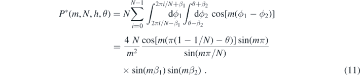
The integral vanishes unless m = 0 or |m| = hN where h is a positive odd integer. We now specialize to the optimal value β1 = β2 = π/(2N), in which case the integrals are π2 and 4 cos[hNθ]/h2, respectively (we evaluated the |m| = hN case by taking the limit of the right-hand side of (11) as |m| → hN). We ignore the θ-independent contribution from the m = 0 term, since it does not lead to a torque on the pendulum.

where δ denotes the Kronecker delta. The total radial integral is a product of integrals R* for the two test-bodies,

that we evaluate using [22, equation 10.22.10],
Integrals of this type appear throughout and so we denote the general case as
In this case, we have
For all of the cases considered below except the IPL interactions, truncating these sums after jmax = 250 gives sufficient accuracy.
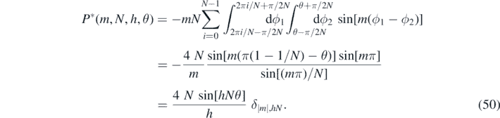
We combine the above integrals where the only non-zero contributions to the energy occur when |m| = hN. The hth harmonic contribution to the energy is

where

is a single infinite integral over k which converges rapidly at large k (see figure 2). The resulting torques are then

The expected torques from Newtonian and Yukawa interactions (assuming α = 1) between our ISL test-bodies are plotted in figure 3.
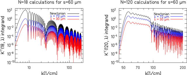
Figure 2. The h = 1 Yukawa energy integrands, see (18), for the 18- and 120-fold test-body geometries of [13].
Download figure:
Standard image High-resolution image
Figure 3. Predicted Newtonian and α = 1 Yukawa torque signals from test-bodies in [13] as a function of s.
Download figure:
Standard image High-resolution image4. Inverse power law potentials
The IPL energy between the two test-bodies, is found by integrating over the source and detector volume:

where  is obtained as follows. We begin with Hobson's equation (23) [23].

where we make the useful substitution (n − 1)/2 → μ.
This is now separable in the z-coordinates of the two points. We apply Gegenbauer's addition formula, equation 10.23.8 in [22], for arguments of Bessel functions satisfying the geometric relationship,  , which applies to all orders of Bessel functions of the first kind,

where  is a Gegenbauer polynomial. When μ = 0, (22) reduces to the familiar Graf addition formula for Bessel functions of order 0 [22, equation 10.23.7],

This result follows from the identities, [24, p 365],

Combining (21) and (22) we have

where


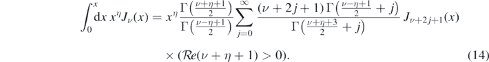
The integration over the vertical coordinates is identical to the Newtonian case ((10) with λ = ∞). We integrate over P(μ, m, ϕ1, ϕ2) by evaluating the Gegenbauer polynomial in (26a) for the special case where μ = 0 using (24). Otherwise, we use the series expansion [22, equation 18.5.11],

Integrating over this expression yields a finite weighted sum of integrals identical to the Newtonian and Yukawa cases ((11), but with m → m − 2q). These integrals are non-zero only if |m − 2q| = hN, i.e. when [m, q] have the values [hN, 0], [hN, hN], [hN + 2, 1], [hN + 2, hN + 1], [hN + 4, 2], [hN + 4, hN + 2], etc.
where δ denotes the Kronecker delta. Finally, as discussed below, it is convenient to move the prefactors  from each of the two radial integrals into the angular integral so that the radial integrals become functions of l = m + 2j alone.
The total radial integral is a product of integrals  for the two test-bodies,

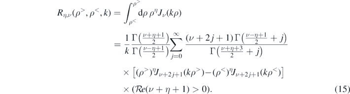
which can be solved using (15) with η = 1 − μ and ν = m + μ so that
For computational efficiency we moved the factor  from the two radial integrals into our definition of P*(μ, m, N, h, θ) so that
Note that R* depends only on the the combination l = m + 2j which substantially speeds up the numerical calculations since a Bessel function of order l may appear many times in the sum over j and m. The first non-zero value of angular integral (29) occurs for l = N; in our application summing over 500 to 3000 non-zero l values provided sufficient precision
The energy associated with the hth harmonic has contributions from all m ⩾ hN
where

Examples of the integrands for the 18-fold and 120-fold test-body geometries are shown in figure 4. The resulting torque is
The expected IPL torques assuming  are plotted for the 18- and 120-fold test-body geometries in figure 5.

Figure 4. The h = 1 power-law energy integrands, see (34), for the 18- and 120-fold test-body geometries in [13]. The n = 1 integrand is nonzero only when |m| = hN, whereas higher order IPLs have contributions from many m's which lead to smoother integrands.
Download figure:
Standard image High-resolution image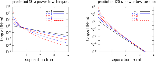
Figure 5. Predicted 18ω and  IPL signals as a function of s from test-bodies in [13].
Download figure:
Standard image High-resolution image5. Spin-dependent potentials
At first sight, it does not seem possible to define similar Green's functions for the dipole-dipole and monopole-dipole potentials given in (4) and (5). However, because these potentials come from derivative couplings of a pseudoscalar [9], we can make the substitutions


5.1. Dipole–dipole interaction
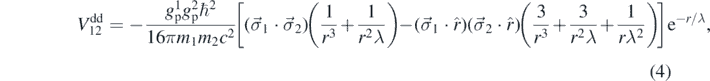
The energy between the two spin-polarized test-bodies is given by (6) with the mass-density differences replaced by  , where dS
is the spin density difference. Since our spin pendulum had azimuthally oriented spins, the energy is
, where dS
is the spin density difference. Since our spin pendulum had azimuthally oriented spins, the energy is
We define

where


The integral over Z(z1, z2, k, λ) is identical to the Newtonian/Yukawa case (10). The integral over (40a) is
The total radial integral is a product of identical integrals for each of the two test-bodies so that

This is an integral of the form in (15) with η = 0 and ν = m, yielding

Combining the above integrals, the energy in the hth harmonic becomes

where

The torque is

The dipole-dipole energy integrands and corresponding torques are plotted in figure 6.
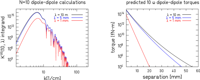
Figure 6. The h = 1 dipole–dipole energy integrands, see (45), at s = 4 mm (left) and the predicted torques (right) assuming gp = ℏc for the 10-fold spin-polarized test-bodies used in [15].
Download figure:
Standard image High-resolution image5.2. Monopole–dipole interaction
The monopole–dipole energy consists of integrals over the pendulum spin-density difference and the attractor nucleon density difference ( )
)

where we define

with


The integral over Z(z1, z2, k, λ) is identical to that in (10). The integral over P(m, ϕ1, ϕ2) becomes
Note that the phase is shifted by 90° relative to the other signals computed here. The radial integral over the attractor coordinates was computed in (16), so that

and the radial integral over the spin-polarized pendulum test-body was computed in (43),

Combining the above integrals, the energy in the hth harmonic becomes

where

and the torque becomes

The monopole–dipole energy integrands and corresponding torques are plotted in figure 7.

Figure 7. The h = 1 monopole-dipole energy integrands, see (54), at s = 4 mm (left) and predicted torques (right) assuming gs = gp = ℏc for the instrument used in [15].
Download figure:
Standard image High-resolution image6. Magnetic systematic interactions
Here we consider the systematic torques arising from the slight magnetization induced in nominally-unpolarized ISL test-bodies by stray external magnetic fields. An external magnetic field generates a polarized spin-density in the direction of the applied field proportional to the magnetic field strength and the test-body volume magnetic susceptibility χv . When the susceptibilities are small, χv ≪ 1, the induced field from one test-body does not appreciably change the spin-density of the other, so that dS = dχ B/(μ0 μe), where μe is the electron magnetic moment, B the external magnetic field strength, and dχ is the difference in the volume magnetic susceptibility of the two elements of the unit-cell. Ignoring irrelevant contact terms, the magnetic vector coupling of photons to electrons gives a spin-dependent potential identical to the dipole–dipole potential of (4) with mϕ = 0 and gp gp → −gV gV = −e2/ɛ0 [9]. The magnetic interaction between electrons is then

We consider the systematic torques from both vertical and horizontal external magnetic fields.
6.1. Vertical magnetization
The energy between vertically magnetized test-bodies is similar to the dipole–dipole interaction of (38) but with a z-oriented spin-density difference

where we define

with


Integration over Z(t1, t2, s, k) becomes

and the integrals over ϕ and ρ are identical to (12) and (16), respectively. So the energy in the hth harmonic is

where

The torque is

Note that a vertical magnetic field produces an attractive interaction that adds to the gravitational torque. The predicted systematic magnetic torques on our ISL instrument [13] due to an external 250 μT vertical magnetic field are plotted in figure 8.

Figure 8. The h = 1 energy integrand, see (62), for the 18- and 120-fold test-body geometries used in [13] (left). Predicted magnetic torques from a 250 μT vertical magnetic field as a function of s (right).
Download figure:
Standard image High-resolution image
6.2. Horizontal magnetization
It is difficult to use cylindrical coordinates to calculate the induced magnetic interaction from a horizontal external magnetic field. However, an analysis in Cartesian coordinates shows that the result differs from the vertical case simply by a factor of (−1/2). Consider two vertically separated rings of N spins evenly spaced in azimuth. Assume that all spins are oriented along x,  , and allow the positions of the lower spins to be rotated by an angle θ. The energy between the sets of N-fold spins is

where the distance between any pair is  . Because these sets of points exhibit cylindrical symmetry, the energy of x-oriented spins is identical to that of y-oriented spins, i.e. Ux
= Uy
. Then we have
. Because these sets of points exhibit cylindrical symmetry, the energy of x-oriented spins is identical to that of y-oriented spins, i.e. Ux
= Uy
. Then we have
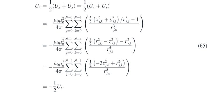
The result is general and applies to any case with cylindrical symmetry. The hth harmonic contribution to the torque between horizontally magnetized test-bodies is then

In this case, the interaction is repulsive and subtracts from the gravitational torque.
7. IPL constraints from the Lee et al data
The Lee et al data [13] consist of m = 18, 54, and 120ω harmonic torques on the pendulum exerted by an attractor uniformly rotating at frequency ω, where the 54ω torque was the third harmonic of the 18ω signal. We extracted IPL constraints from these data using a procedure nearly identical to that used to exclude Yukawa potentials [13]. We fit our torque measurements, Tm, accounting for systematic errors in measured position and other experimental parameters ( and
and  , respectively), by minimizing the χ2 function

where  for n ∈ [2, 3, 4, 5], and where δsj
was the uncertainty in the separation measurement. We found none of the fits for additional IPL potentials improved the χ2 by 2σ (Δχ2 = 2) over the pure Newtonian fit. We placed 68% confidence limits on each, improving slightly on the work of [25] for n = 5, see table 1.
for n ∈ [2, 3, 4, 5], and where δsj
was the uncertainty in the separation measurement. We found none of the fits for additional IPL potentials improved the χ2 by 2σ (Δχ2 = 2) over the pure Newtonian fit. We placed 68% confidence limits on each, improving slightly on the work of [25] for n = 5, see table 1.
Table 1. 68% confidence limits from laboratory constraints of power law potentials from this work and [25].
| n |
 (this work) (this work) |
 (reference [25]) (reference [25]) |
|---|---|---|
| 2 | 1.4 × 10⁻³ | 3.7 × 10⁻⁴ |
| 3 | 2.5 × 10⁻⁴ | 7.5 × 10⁻⁵ |
| 4 | 4.3 × 10⁻⁵ | 2.2 × 10⁻⁵ |
| 5 | 6.3 × 10⁻⁶ | 6.7 × 10⁻⁶ |
We verified several of our derivations using commercial symbolic math software [26], and our calculations at several separations were checked against a simulation using discretized test-bodies [27]. The software used to calculate IPL torques, POWERLAW, and Fourier-Bessel torques, FBESSELN, are both available on request from the corresponding author.
8. Summary
We provided details of the powerful and efficient analytical techniques used to optimize the design and the analysis of the results of two quite different experiments: short-range gravity experiments by Lee et al [13], and the search for short-range spin-dependent forces by Terrano et al [15]. We extended the analysis to include IPL potentials and used this to extract limits on such interactions from the Lee et al data. These limits confirm constraints placed by Tan et al [25] and improve slightly on inverse 5th-power law potentials. We also considered the systematic effects of weak external magnetic fields on the nominally-unpolarized test-bodies used in [13]. The results are in quantitative and qualitative agreement with the data [20].
Acknowledgments
This work was supported by NSF Grant No. PHY-1912514 and builds upon previous work by the authors.
Data availability statement
The data that support the findings of this study are available upon reasonable request from the authors.