Optimized loss function in deep learning profilometry for improved prediction performance

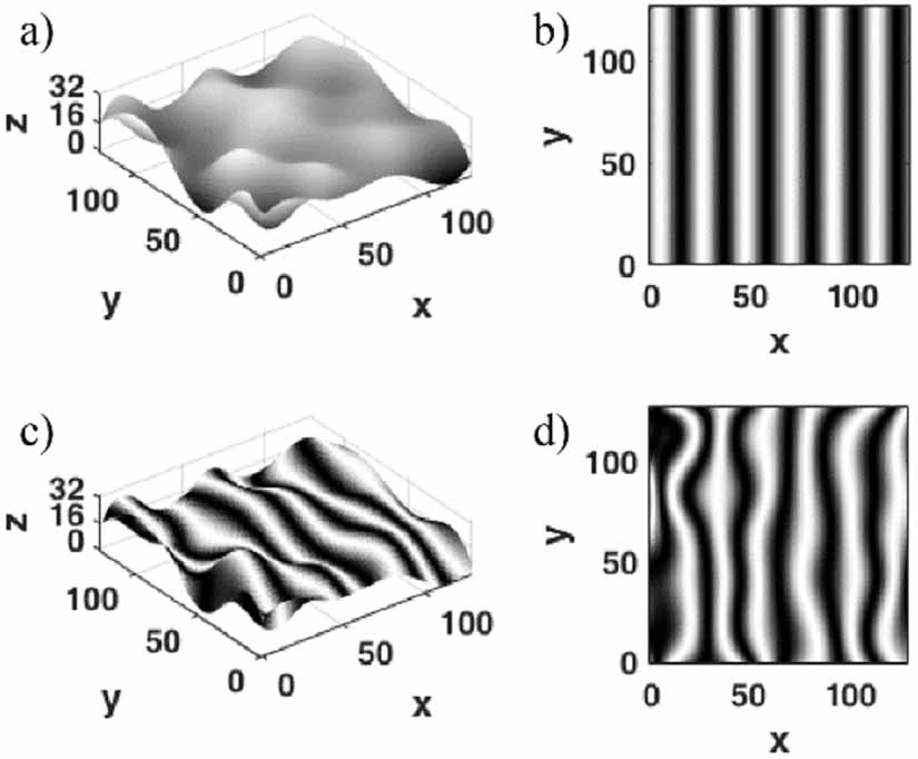
We use a dataset of simulated height maps with corresponding deformed fringe patterns as data couples to train the neural network. To automate the process of constructing a large training dataset, a random surface map generator is designed. Input parameters such as boundary limits, number of peaks, and sharpness or smoothness of the edges can all be set and are randomly varied within predefined limits to produce a set number of randomly varying 3D height maps. Reflectivity is assumed to be uniform and no additional noise is added to the simulated fringe maps. After the creation of a set of randomly fluctuating height maps, a predefined fringe pattern is projected virtually onto each height map and the resulting surface modulation is observed under a fixed angle α. Using straightforward triangulation, the modulated fringe pattern is sampled on a Cartesian grid. The complete process of data-couple generation is illustrated in figure 1.

Zoom In Zoom Out Reset image size

The simulated dataset used in this work aims to mimic images obtained with real SLP setups. Consequently, realistic values for fringe pattern frequency (six periods per image width), the angle between projection and observation axes (α = 30°), and maximum width to height ratio (4:1) are chosen in the generation of our dataset. $Z$-values were confined to $z \in {\mathbb{R}^3}\left[ {0,32} \right]$. Note that the maximum $z$-value of 32 does not necessarily need to be attained for every surface map; it is simply the upper limit. The 4:1 ratio between image width and maximum surface height reduces the amount of shadows that may arise during the fringe modulation process. Deformed fringe patterns and height maps are each sampled on a grid of 128 × 128 pixels. After fringe modulation, volumetric boundary limits of the surface maps in our dataset are normalized to $x,y,z \in {\mathbb{R}^3}\left[ {0,1} \right]$. For a more detailed description of the training data set generation, we refer the reader to [8].

The neural network employed in this work is a modified version of the U-net proposed by Ronneberger et al [21]. A schematic representation of its architecture is shown in figure 2. The modified U-net can be divided symmetrically into a contracting path (encoder) and an expansive path (decoder). The contracting path consists of a succession of convolutional layers with 5 × 5 filters, each followed by a rectified linear unit (ReLu) activation function. After every two successive convolutional layers, a 2 × 2 max-pooling operation is applied. Together, two convolutional layers and one max-pooling layer form a downsampling block. Each downsampling block halves the spatial size of the input representation but doubles the number of feature maps, starting with four feature maps for the first block, eight for the second, and so on. The purpose of the contracting path is to capture the context of the input image by increasing the receptive field of the feature maps. By doubling the number of feature maps with each downscaling block, the architecture can detect the complex structures that are present in the input image more efficiently [22]. The expansive path is symmetrically identical to the contracting path, except that the max-pooling operations are replaced by a 2 × 2 deconvolutional layer that precedes the convolutional layers in each upsampling block. The deconvolutional (or transposed convolutional) layers upsample the input feature map by a factor of 2. With each deconvolutional operation, the number of feature maps is halved until finally a single convolutional layer with a 1 × 1 filter is applied to the output of the last upsampling block. By using a symmetric network architecture, the modified U-net produces an output image of identical size as the input image.

Zoom In Zoom Out Reset image size

Note that each upsampling block has access to the output feature map of its corresponding downsampling counterpart through concatenated skip connections between them. This allows the expansive path to reuse the previously learned local features, allowing information to be retained directly from previous layers of the network. In total, our model contains 78 997 free parameters.

2.3.1.  ${L_1}$ and ${L_2}$

Single-shot deep learning-based profilometry aims to learn a mapping function $\hat Y = f\left( X \right)$ that transforms a 2D modulated fringe map ($X$) to a continuous 3D height distribution ($\hat Y$) without any additional intermediary processing steps. The loss function is the metric that defines how close the predicted height map $\hat Y$ is to the ground truth $Y$. Common metrics that are used as loss function in the training of neural networks are ${L_1}$ or mean absolute error (MAE) and ${L_2}\,$or MSE:

$$\begin{equation}{L_1}\left( {y,\,\hat y} \right) = \frac{1}{n}\mathop \sum \limits_{i = 1}^n \left| {\widehat {{y_i}} - {y_i}} \right|\end{equation} \tag{ 2 }$$

$$\begin{equation}{L_2}\left( {y,\,\hat y} \right) = \frac{1}{n}\mathop \sum \limits_{i = 1}^n {\left( {\widehat {{y_i}} - {y_i}} \right)^2}\end{equation} \tag{ 3 }$$

with $n$ the number of data points. From their definitions, some properties of ${L_1}$- and ${L_2}$-norms can be deducted when they are used as loss function in deep learning models. First, it can be seen that ${L_2}\,$is more sensitive to outliers in the dataset compared to ${L_1}\,$since the differences between prediction and ground truth are squared. As a result, ${L_2}$ will adjust the model to minimize the error caused by these single outlier cases at the expense of many other data points if they contribute only little to the general error. On the other hand, ${L_1}$-norms produce less stable solutions, meaning that for a small horizontal adjustment of a single data point the slope of the regression line between data samples may jump a large amount. Selection between ${L_1}\,$and ${L_2}$-norms as loss function of choice in a deep learning model is made primarily based on this trade-off between robustness and stability and which of these properties is more desirable for the given minimization problem.

2.3.2. SSIM and MS-SSIM

The structural similarity index (SSIM) is a metric that is frequently used as loss function in single-image super-resolution models [23] and other tasks that involve human perceptual judgment. The SSIM and its multi-scale variant MS-SSIM are loss functions that, unlike ${L_1}$ and ${L_2}$, are based on the human visual system as they aim to match the luminance $I$, contrast $C,\,$ and structural information $S$ between images. The SSIM is defined as:

$$\begin{equation}{\text{SSIM}}\left( {y,{ }\hat y} \right) = I{\left( {y,{ }\hat y} \right)^\alpha }C{\left( {y,{ }\hat y} \right)^\beta }S{\left( {y,{ }\hat y} \right)^\gamma }\end{equation} \tag{ 4 }$$

with

$$\begin{equation*}I\left( {y,\,\hat y} \right) = \frac{{2{\mu _y}{\mu _{\hat y}} + {C_1}}}{{{\mu _y}^2 + {\mu _{\hat y}}^2 + {C_1}}}\end{equation*}$$

$$\begin{equation*}C\left( {y,\,\hat y} \right) = \frac{{2{\sigma _y}{\sigma _{\hat y}} + {C_2}}}{{{\sigma _y}^2 + {\sigma _{\hat y}}^2 + {C_2}}}\end{equation*}$$

$$\begin{equation*}S\left( {y,{ }\hat y} \right) = \frac{{{\sigma _{y\hat y}} + {C_3}}}{{{\sigma _y}{\sigma _{\hat y}} + {C_3}}}.\end{equation*}$$

The variables ${\mu _y}$, ${\mu _{\hat y}}$, ${\sigma _y}$ and ${\sigma _{\hat y}}$ denote mean pixel intensity and standard deviations of pixel intensity in a local image patch at either $y$ or $\hat y$, respectively. In the following, we choose a square region of 3 pixels on either side of $y$ or $\hat y$, which results in patches of 7 × 7 pixels. The variable ${\sigma _{y\hat y}}$ denotes the sample correlation coefficient between corresponding pixels in the patches centered at $y$ and$\,\hat y$. The constants ${C_1}$,$\,{C_2}$ and ${C_3}$ are small constant values that are added for numerical stability and $\alpha$, $\beta$ and $\gamma$ define the weights given to each component of the SSIM.

The SSIM metric assumes a fixed image sampling density and is a single-scale index. An extension to this metric is the multi-scale variant MS-SSIM, which can operate at multiple scales simultaneously. The ground truth image $y$ and its candidate approximation image $\hat y$ are both iteratively downsampled by a factor of 2. The contrast $C$ and structural $S$ components are applied at all scales. The luminance component $I$, however, is only applied at the coarsest scale, denoted $M$. Again, the weighting of the different components is allowed at each scale, leading to the following definition of the MS-SSIM:

$$\begin{equation}{\text{MS-SSIM}}\left( {y,\,\hat y} \right) = {I_{\text{M}}}{\left( {y,\,\hat y} \right)^\alpha }\mathop \prod \limits_{j = 1}^M {C_j}{\left( {y,\,\hat y} \right)^{{\beta _j}}}{S_j}{\left( {y,\,\hat y} \right)^{{\gamma _j}}}.\end{equation} \tag{ 5 }$$

Note that both SSIM and MS-SSIM are normalized to $\left[ {0,1} \right]$ where 1 indicates a full correspondence between $y$ and $\hat y$. Since the loss function employed in a neural network is to be minimized, we use 1–SSIM and 1–MS-SSIM instead.

2.3.3. Mean gradient error (MGE) and mixed gradient error (MixGE)

In SLP, we are mainly concerned about relative phase differences. Two surface shapes can be assumed to be identical if their pixel-wise phase difference is a constant value: subtracting the minimum, mean or maximum value of the surface map from each pixel value suffices to unwrap the phase map of dynamically moving surface shapes temporally. It, therefore, makes sense to incorporate the local gradient of the prediction ($\hat Y$) and the ground truth ($Y$) surface maps directly into the loss function. Inspired by [24], we introduce classic gradients to the loss function using Sobel operators:

$$\begin{equation*}{G_x} = Y*\,\left[ {\begin{array}{*{20}{c}} { - 1}&0&1 \\ { - 2}&0&2 \\ { - 1}&0&1 \end{array}} \right]\end{equation*}$$

$$\begin{equation*}{G_y} = Y\,*\,\left[ {\begin{array}{*{20}{c}} { - 1}&{ - 2}&{ - 1} \\ 0&0&0 \\ 1&2&1 \end{array}} \right]\end{equation*}$$

where $*$ denotes the convolution operator. Together, the gradients ${G_x}$ and ${G_y}$ are combined into the general pixel-wise gradient map $G = \sqrt {{G_x}^2 + {G_y}^2}$. Likewise, the gradient map $\,\hat G$ of the predicted surface map $\hat Y$  can be calculated. The MGE can then be defined as:

$$\begin{equation*}{\text{MGE}} = \frac{1}{n}\frac{1}{m}\mathop \sum \limits_{i = 1}^n \mathop \sum \limits_{j = 1}^m {\left( {G\left( {i,j} \right) - \hat G\left( {i,j} \right)} \right)^2}.\end{equation*}$$

Using the MGE directly as a stand-alone loss function of the neural network would result in divergence of the model since the DC component is completely removed from the solution. The MGE can, however, be used as an auxiliary component by adding it to the standard ${L_1}$-norm in the creation of a MixGE:

$$\begin{equation}{\text{MixGE}} = \left( {1 - \lambda } \right){L_1} + \lambda {\text{ MGE}}\end{equation} \tag{ 6 }$$

where $\lambda \in \left[ {0,1} \right]$ is the gradient error weight factor that needs to be optimized in function of the employed model architecture and dataset.

To train our network, a dataset of N_total = 12 500 simulated data couples is created using the automated surface generator. The number of local surface maxima and minima that are present in the simulated height maps varies randomly between 0 (flat planes of random height) and 15 (highly fluctuating landscapes). Either linear or spline interpolation is used randomly to sample the simulated surfaces on a 128 × 128 grid between the minima and maxima, resulting in a mix of surface maps containing both sharp and smooth edges, respectively. A training dataset of N_train = 10 000 simulated input-output pairs is used to train the network and a validation dataset of N_val = 2500 simulated input-output pairs is used to test the performance of the model on previously unseen data.

The Tensorflow framework [25] is used to train the modified U-net. The batch size is set at 4 and roughly 100 full passes (or epochs) through the training dataset are completed, depending on the individual convergence of the network trained with each employed loss function. We use Adam optimization with an initial learning rate of 10⁻⁴. Before training, the initial values of the filter weights are set using Xavier initialization to ensure equal variance between successive layers. To regularize training and to reduce overfitting, L₂ weight decay is used with an initial setting of 10⁻³. After every 50 000 iterations, the learning rate is divided by 5, and L₂ penalties are divided by 10. During the final set of iterations, L₂ penalties are set to 0. The number of training iterations was chosen so that for each loss function investigated in this paper (${L_1}$, ${L_2}$, SSIM, MS-SSIM, and MixGE), the validation error reached convergence. Convergence is defined here at the point where the validation error does not improve for five consecutive epochs. In addition, validation curves are monitored to confirm the general converging behavior of the network and to ensure that no faulty divergence is occurring. Our implementation uses cuDNN and is optimized for parallel execution. The training time of a single model varies depending on the employed loss function. In total, the training time for a single model ranges between 34 min (MAE), 35 min (MSE), 36 min (MixGE), 42 min (SSIM), and 62 min (MS-SSIM) when deployed on a Titan X Pascal GPU. These convergence times correspond to a total number of training epochs of 98, 102, 92, 106, and 119 for networks trained using ${L_1}$, ${L_2}$, MixGE, SSIM, and MS-SSIM, respectively.

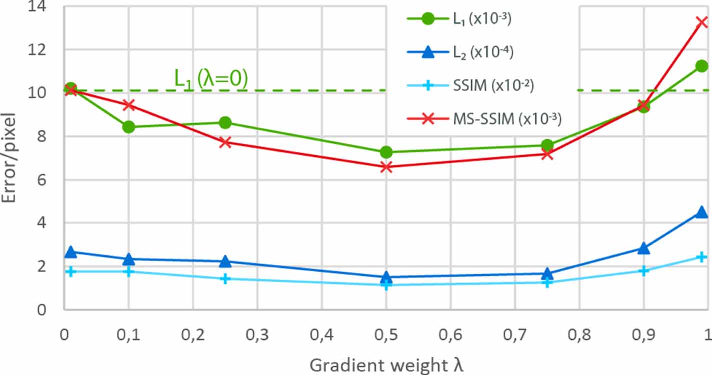
First, the modified U-net model was trained using various ratios of MGE/${L_1}$ to find the optimal contribution of the MGE component to the total MixGE. Several values of $\lambda$ ranging from 0 to 0.99 were used in equation (6) to modify the impact of the MGE component. Each resulting MixGE loss function was used to train the model to convergence on a fixed dataset. Upon convergence, the model performance was evaluated on the validation data set using the ${L_1}$,$\,{L_2}$, SSIM, and MS-SSIM metrics. The result is shown in figure 3. The models trained with the MixGE outperform those trained with standard ${L_1}$ loss up to a value of $\lambda$ ≈ 0.95. Beyond this point, the MGE component becomes too dominant over the DC component provided by ${L_1}$, resulting in divergence of the model and a steep increase in prediction error. Although the various metrics provide different evaluations of the models trained using the differently weighted MixGE loss functions, they all reach a minimum error per pixel when $\lambda$ is chosen between $\lambda$ = 0.40 and $\lambda$ = 0.60. In the following, we will use a gradient weight of $\lambda$ = 0.50 in the MixGE loss function.

Zoom In Zoom Out Reset image size

The modified U-net was trained to convergence using each of the ${L_1}$, $\,{L_2}$, SSIM, MS-SSIM, and MixGE loss functions. The performance of each trained model was evaluated by comparing the height map predictions ($\hat Y$) of the samples in the validation set to their respective ground truth ($Y$) height maps using each of the corresponding metrics of ${L_1}$, $\,{L_2}$, SSIM, MS-SSIM, and MixGE. The resulting error values were averaged over the entire validation set and are included in table 1.

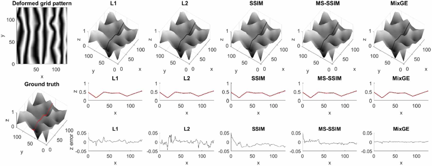
The top part of table 1 (General) represents the performance matrix over the entire validation dataset, containing 2500 simulated height map samples with a random mix of both smooth (spline-interpolated) and sharp (linearly interpolated) edges. The MixGE loss function outperforms the other loss functions on this general population of height maps by a significant margin, even when the evaluation metric is the same as the one that was used as loss function in the training of the model. Only when the MS-SSIM metric is used, the model trained with the MixGE loss function is scored second best after the MS-SSIM loss function itself. Top performing metric is underlined.

To further investigate the effect of surface shape variation on loss function performance, two additional validation datasets of each N = 1000 data couples were created using the random surface map generator: one in which only spline interpolation was used to connect the peaks and troughs present in the height map, and one in which only linear interpolation was used. From the middle and bottom parts of table 1, a large discrepancy can be observed between ${L_2}$-performance on samples with smooth edges (Spline) and those with sharp edges (Linear). For all metrics, ${L_2}$ performs significantly worse on surfaces with sharp edges than it does on surfaces with smooth edges. This behavior is reflected in the samples illustrated in figures 5 and 6. Whereas models trained with ${L_1}$, SSIM, MS-SSIM, and MixGE loss functions perform similarly on spline-interpolated height maps (figure 4) as on linearly interpolated height maps (figure 5), the model trained with ${L_2}$-loss produces a larger error when applied to predict height maps with sharp edges than when applied to predict height maps with smooth, curved edges.

Zoom In Zoom Out Reset image size

Zoom In Zoom Out Reset image size

Zoom In Zoom Out Reset image size

To highlight the superior performance of MixGE over the other loss functions, we include the measurement of the surface shape of a mannequin doll head in figure 6. The ground truth 3D surface measurement was obtained using four-step phase-shifting profilometry. Parts of the surface map where shadows, saturated reflections or any other regions of invalid data corrupted the 3D measurement were interpolated in post-processing. It can be seen that the model trained with MixGE does a significantly better job of predicting the mannequin doll surface shape than the models trained with the other loss functions. It should be noted that a clear linear error is present across all prediction maps, including the one reconstructed with the MixGE loss. This may be due to the strong localized height variations near and above the eye region of the mannequin head model. In the training dataset, no samples with such relatively large jumps in Z-value have been included and none of the loss functions seem to handle these properly.

Finally, to assess how the different loss functions are influenced by the presence of noise in the fringe patterns, an additional validation set of N = 1000 data couples was generated in which each input fringe map contained Poisson noise with the pixel value as the mean (before normalization). The corresponding error matrix is included in table 2 and a random sample from the validation set is shown in figure 7. First of all, it can be seen that the models trained with the ${L_1}$, ${L_2}$ and MixGE loss functions are able to extract the general form of the 3D map sufficiently well. As the neural network was trained to produce smooth, noise-free surface maps only, the predicted height maps are largely noise-free even when the input maps themselves are not. This way, noise filtering is implicitly learned by the network. The models trained with the SSIM-based losses, however, are more affected by the increased noise level. It should be noted that we assess 'pure' SSIM loss-prediction accuracy here: a mixed loss function containing an additional contribution of ${L_1}$- or ${L_2}$-loss might alleviate this oversensitivity to the added shot noise of the SSIM-family of loss functions. It can be seen from table 2 that MixGE outperforms all other loss functions by a significant margin.

Zoom In Zoom Out Reset image size