

Abstract
We analyse the dynamics of a network of semiconductor lasers coupled via their mean intensity through a non-linear optoelectronic feedback loop. We establish experimentally the excitable character of a single node, which stems from the slow-fast nature of the system, adequately described by a set of rate equations with three well separated time scales. Beyond the excitable regime, the system undergoes relaxation oscillations where the nodes display canard dynamics. We show numerically that, without noise, the coupled system follows an intricate canard trajectory, with the nodes switching on one by one. While incorporating noise leads to a better correspondence between numerical simulations and experimental data, it also has an unexpected ordering effect on the canard orbit, causing the nodes to switch on closer together in time. We find that the dispersion of the trajectories of the network nodes in phase space is minimized for a non-zero noise strength, and call this phenomenon canard resonance.
Export citation and abstract BibTeX RIS

Original content from this work may be used under the terms of the Creative Commons Attribution 4.0 license. Any further distribution of this work must maintain attribution to the author(s) and the title of the work, journal citation and DOI.
1. Introduction
Neuromorphic photonics has recently emerged as a key area of research in which multiple goals can be pursued. On the one hand, leveraging complex photonic dynamics for data processing is promising in view of realizing energetically efficient photonic computing platforms. On the other hand, photonics has long served as a hardware platform for the exploration of complex dynamics (for a review see [1]). The main dynamical characteristic of a neuromorphic node is excitability; thus, most experimental studies have focussed on the analysis of the excitable properties of single (or a few coupled) lasers and optical devices [2–19].
Excitable systems possess a stable attractor (rest state) which can be forced to spike by stimuli of amplitude above a given threshold. Each pulse is associated with a well-defined orbit in the phase space that is barely dependent on the detailed nature of the stimulus and during which the system is insensitive to any new, above-threshold, perturbation (refractory time).
In many cases, in particular when the rest state is near a Hopf bifurcation, excitability results from the competition of multiple time scales [20], and the phase space orbit is characterized by the existence of a slow invariant manifold consisting of attracting and repelling parts. This is paradigmatically illustrated by the FitzHugh–Nagumo model, originally introduced as a simplified description of neural activity [21, 22]: the excitable orbit can be decomposed into periods of slow motion, taking place near the attractive branches of a cubic critical manifold, separated by fast relaxations between them [23]. However, in particular conditions, and typically for an exceedingly small parameter range, the trajectories may spend a considerable amount of time moving on a slow timescale along the repelling part of the manifold, instead of quickly departing from it. These special trajectories are known as canard orbits [24, 25] and in higher-dimensions are at the basis of complex oscillatory dynamics [26–31]. The canard trajectories show an extreme sensitivity to the control parameters and to fluctuations (either of deterministic or stochastic nature): noise can give rise to a marked variability of the excitable orbit and may therefore have a huge impact on the system dynamics.
Yet, direct observations of canard trajectories are not so frequent, in particular in optics. Canard explosions have been described recently in semiconductor lasers, for instance in [32]. Regimes of chaotic canard explosions characterized by irregular spike-sequences produced after period-doubling cascade of subthreshold oscillations have been reported in [33]. Notably, on each point of the cascade the system is excitable, thus extending the concept of excitability (typically associated to fixed points) also to the case of higher-dimensional attractors. These regimes have been experimentally observed in semiconductor lasers with opto-electronic feedback [34, 35] and, later on, in optomechanical resonators [36, 37].
In networks of non-identical excitable or oscillatory elements, the interplay between noise and nodes heterogeneity produces a stochastically-enhanced coherence of the canard trajectory, a phenomenon that we name canard resonance and analyse numerically in this work.
The role of noise in excitable systems, at the level of stochastic entrainment of pulses, has been widely investigated [38]. It is well known that a finite amount of noise in non-linear systems may induce a dynamical state which is, according to some indicator, more ordered [39–42]. Two examples of such noise-induced-ordering phenomena are the so-called stochastic resonance [43] and coherence resonance [44, 45]. In both cases the key concept is the interplay between a stochastic timescale, fixed by the noise variance, and a deterministic timescale. Stochastic resonance refers to a situation in which the system exhibits the maximum correlation with an applied periodic signal for an optimal value of the noise amplitude. In excitable systems, the spiking occurs periodically at the frequency imposed by the modulation, evidenced by a peaked inter-spike interval (ISI) distribution [46, 47]. On the other hand, nearly periodic sequences of excitable spikes may arise for an optimum noise amplitude even in the absence of external periodic forcing: this is the case of coherence resonance. The effect has been theoretically studied also in bursting systems [48–50] and has been demonstrated experimentally in different physical setups [51–53]. In addition to coherence resonance, even the inverse phenomenon of stochastic incoherence has been reported, showing that in excitable systems there exists a range of noise amplitudes at which a resonant, increased variability in the ISIs can be observed [54]. This has been shown in leaky integrate-and-fire neurons [54], in the FitzHugh–Nagumo model [55] and in bursting systems [56].
Noise-ordering effects have been also investigated in networks of excitable elements [38]. In particular, coherence resonance has been reported in heterogeneous arrays of coupled FitzHugh–Nagumo neurons, showing that the coupling leads to a stronger coherence compared to that of a single element [57]. Interestingly, the inhomogeneity of the nodes enhances the coherence of the spikes sequence [58]. These phenomena have been analysed in models of coupled semiconductor lasers with saturable absorber in [59]. Similar effects have been analysed in coupled FitzHugh–Nagumo models [60, 61] and experimentally observed in two coupled chaotically-spiking systems [62].
Here, we investigate a different phenomenon in which the stochastically-induced coherence does not appear in the ISI distribution, but emerges in the form of a 'resonant' canard trajectory for a finite amount of noise in a parameter regime in which the deterministic dynamics is periodic. We analyse these effects in a globally coupled network of hundreds of semiconductor lasers with optoelectronic feedback, which collectively display a spiking canard similar to that observed in a single-laser [34]. The above dynamics that is effectively low dimensional, is determined from the existence of a critical manifold consisting of a bundle of 1D branches, which for nearly identical nodes closely resemble that of the single laser [63]. The canard resonance is due to the interplay of noise and such composite manifold structure.
We present the experiment and the scaled theoretical model in section 2. In section 3 we analyse experimentally and numerically the excitable character of a single node. Section 4 is dedicated to the analysis of the critical manifold structure, which can to some extent be detected experimentally. In section 5, we focus our numerical study on the role of noise (which must evidently be incorporated to properly describe the experiment) and in particular on the numerical observation of the canard resonance. Finally we summarize our results in section 6.
2. Experiment and model
2.1. Experimental setup
The experiment, inspired by [34, 35], is based on a semiconductor laser array subject to optoelectronic feedback, as shown on figure 1. The laser array consists of 451 Vertical Cavity Surface Emitting Lasers (thus single longitudinal mode), all biased by a single power supply. The average laser threshold of the population is 183.3 mA with a standard deviation of 5.8 mA (more details are available in [63, 64]). Due to the spectral distribution of the lasers (the array's spectrum is 2 nm broad), coherent coupling via field interaction can be neglected. In fact, far field measurements show no sign of interference between the individual lasers. The beam emitted by the laser array is collected by a short focal length lens and split in a detection and a feedback branch. In an image plane along the feedback branch (marked as 'NF' in figure 1), an iris whose aperture and position can be controlled allows to select the part of the array which will be guided further towards the feedback detector. On this path, a clippable mirror can send the beam towards a rotating screen for image analysis in absence of feedback. The selected part of the beam is focussed onto a photodetector (photodetector 1 in figure 1). The voltage produced by this detector is proportional to the total intensity emitted by the region of the array selected by the iris. This voltage is logarithmically amplified and its continuous component is suppressed. After a final linear amplification stage it is injected as a controller for the power supply driving the whole array. This leads to a global coupling through the optoelectronic reinjection. The detection branch is split in two by a prism situated in an image plane (labelled 'NF') on figure 1 and parts of each of these beams can be selected by two additional iris. Each of the selected beams are then focussed on two independent detectors which enable monitoring of parts of the whole network down to the single element. Additional details can be found in [64].
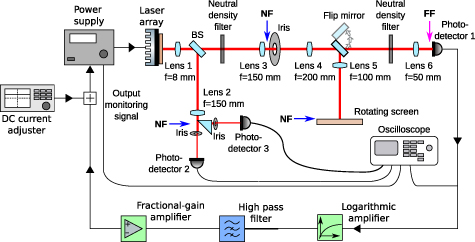
Figure 1. Experimental setup of a laser array with non-linear opto-electronic feedback. The beam emitted by a laser array is split in detection and feedback branch. The feedback branch is sent towards a photodetector (photodetector 1) whose voltage is logarithmically amplified, high-pass filtered and linearly amplified before being re-injected in the drive voltage of the laser power supply. Lenses are used to form images of the array in the planes labelled 'NF' so that parts of the beam can be collected by several iris.
Download figure:
Standard image High-resolution image2.2. Scaled model
We consider the following adimensional model for a population of N coupled lasers, subject to optoelectronic feedback. The model in physical variables together with the scaling is fully described in [63, 64]
where xi
(t) is the normalised intensity and yi
(t) is the normalised carrier density of each laser, and time is normalised to the photon lifetime. The variable w(t) represents the scaled high-pass filtered feedback current, and is common for the whole population. This feedback depends nonlinearly on the mean intensity  : the lasers are coupled in an all to all configuration through the feedback. The lasers differ by their lasing thresholds, and thus by their relative pump currents δi
. We order the lasers in descending order of their pump currents; i.e.
: the lasers are coupled in an all to all configuration through the feedback. The lasers differ by their lasing thresholds, and thus by their relative pump currents δi
. We order the lasers in descending order of their pump currents; i.e.  The parameter k represents the coupling strength and A and α are the parameters of the non-linear saturable absorber in the high-pass filtered feedback current. The timescales of the system depend on the ratio of photon and carrier lifetimes
  , and
, and  , which relates to the feedback filter.
We integrate noise in equations (1) in a way similar to spontaneous emission noise, as an additive noise term added to the evolution of the complex laser electric field Ei
(t),  ,
,

where ξi (t) are independent white gaussian complex noise terms with zero mean and unit variance, and σ is the noise strength. We use 2 whose deterministic part is equivalent to that of the equation for x in 1 because in 2 the simple zero-mean complex noise term adequately captures the spontaneous emission process, which is less convenient to express in terms of the intensity x. The linewidth enhancement factor αH does not play a role in the dynamics of this system, but is added for completeness. We chose αH = 4 in all simulations with noise. Of course, a proper description of all noise sources in semiconductor lasers leading to accurate modeling of spectral lineshapes or relative intensity noise spectra would require additional stochastic terms (see e.g. [65–67]). However, here we only aim at introducing a minimal yet physically meaningful stochastic term and at observing its impact on the canard trajectories.
We use an Improved Euler algorithm incorporating additive noise, with a time step of dt = 0.1. In our simulations, we have always used the timescale parameters γ = 4 · 10−3 and  = 10−4, and feedback parameters
  and α = 2, unless otherwise mentioned, as these parameters reproduce the experimental results qualitatively. Sample checks performed using the stochastic Runge–Kutta algorithm described in [68] implemented by [69] did not show any inconsistencies.
3. Single node dynamics
3.1. Theoretical phase space structure
The experimental setup is built to mimic neural dynamics; the neuromorphic laser can show excitable, oscillating and chaotic dynamics, depending on the parameters. We briefly review [63, 64] the dynamics of a single node (N = 1, X(t) = x1(t)≡x(t)) in order to facilitate comparison with the dynamics of the population. The system is a slow-fast system with being the slowest timescale in the system. The critical manifold, defined by = 0, has two branches. The OFF-branch is defined by

the motion on the OFF-branch is towards the non-lasing fixed point at  . The OFF-branch is attracting for
  , the non-lasing fixed point is stable if
  . The ON-branch is implicitly defined by

the motion is towards the lasing fixed point at  . The ON-branch emerges at
  and is attracting for
  or, equivalently,
  . The critical manifold is shown in figure 2(c).
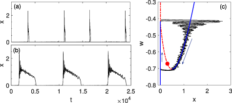
Figure 2. Single node dynamics and phase space structure. Noise-triggered excitable pulses are visible for δ = 0.995, σ = 5 × 10⁻³ (a). For the same noise strength, regular spiking oscillations appear at higher δ (here δ = 1.3, (b)). (c) Two-dimensional projection of the dynamics in the (x, w) plane for δ = 1.3, σ = 5 × 10⁻³. The critical manifold is shown: full blue lines are attracting parts, dashdotted red lines are repelling. The unstable lasing fixed point is also indicated as a red dot. The arrows indicate the direction of the trajectory on the two branches of the slow manifold. The oscillatory nature of the transient is enabled by the existence of an intermediate time scale.
Download figure:
Standard image High-resolution imageThus, the dynamics is excitable if  : The non-lasing fixed point is stable but the system responds to perturbations either by relaxing linearly back to the original state or, if the perturbation overcomes a certain threshold, by undergoing a large excursion (mostly independent of the details of the perturbation) in phase space due to the very different time scales. In particular, noise may drive the laser away from the OFF-branch; if the system reaches the ON-branch, a spike is emitted. The excitable dynamics is shown in figure 2(a), where noise triggers the random emission of excitable pulses.
The lasing fixed point is stable for  , and the dynamics are excitable as well. The fixed point undergoes a Hopf bifurcation as δ decreases, followed by a period doubling cascade and the emergence of a strange attractor with small amplitude. As this attractor grows in size, the critical manifold becomes part of it, and the system emits a large spike on top of the small amplitude chaotic dynamics. This chaotic region only exists for a small parameter range around
  .
.
For  none of the fixed points is stable. The neuromorphic laser exhibits, depending on the pump current δ, chaotic or regular spiking oscillations, as the system alternates between the two branches. Importantly, while the periodic alternation between the two branches is common to many planar slow-fast system, the chaotic dynamics and oscillatory jumps between these branches are enabled by the presence of a third intermediate time scale. The regular spiking regime, which is the focus of our numerical study, is illustrated in figures 2(b) and (c).
3.2. Experimental observation of excitability threshold
From the analysis above, one expects two parameter regions leading to excitable behaviour. We concentrate experimentally on the first one, where the laser is in a stable non-lasing state.
To check this behaviour, we close the population control iris such that only the part of the beam emitted by a single laser is actually transmitted towards the feedback detector. In this configuration, the other lasers are slaved to the dynamics of the selected one and the system can be analysed as a single node. While additional coupling between lasers (mostly through gain medium or thermal dynamics) could exist, we have no evidence of these effects taking place here and therefore analyse our results in the framework set by the model where the only coupling is through the optoelectronic reinjection. We focus on the response of the system to external perturbations when it is biased below its coherent emission threshold and close to the first instability. We direct towards the feedback detector a beam coming from another semiconductor laser emitting at 970 nm. The current of that laser is pulsed so that optical pulses of 40 µs duration are emitted at a repetition rate of 10 Hz. We apply stronger and stronger light pulses from that laser onto the feedback detector and monitor the response of the system. The results are shown in figure 3.
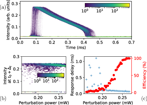
Figure 3. Excitable response of a single laser with optoelectronic feedback. Top: superposition of 103 responses to optical perturbations of 0.22 mW. The logarithmic color scale shows the response distribution. Bottom left: emitted intensity at a prescribed delay Δt after the perturbation is sent to the system. Bottom right: large response delay (blue crosses) and efficiency (red disks) of the perturbation in generating these large responses. Array pump DC current: 176.3 mA. At this current, the specific laser selected by the iris is below its standalone threshold and only about 1 mW (spontaneous emission) reaches the feedback detector.
Download figure:
Standard image High-resolution imageFor small perturbations, below 0.2 mW approximately, the system's response is almost always linear with only very rarely a large spike response. On panel (a) of figure 3, we show a superposition of 103 responses to perturbations of 0.22 mW. The perturbations are applied at a repetition rate of 10 Hz, low enough that all realizations can be considered as independent. At this power value, about half of the perturbations elicit a large spike response. The latter arise after a small and variable delay as show by the dispersion on the rising edge. To confirm the only two possible responses, we plot on panel (b) of figure 3 the mean intensity emitted in a short time window of duration 0.1 ms at a time Δt = 0.1 ms after the perturbation signal has been emitted, for increasing perturbation power. Only two regions are often visited by the system. The bottom one, close to 0.02 arb.units corresponds to the linear response and the top one, close to 0.25 arb.units corresponds to the excitable orbit. These two regions are clearly separated by the large empty area in the diagram, which shows that either a linear response or a large response can be emitted. The former is most probable for low perturbation power and the latter is strongly dominant for large perturbation power. We quantify the efficiency in the generation of these excitable responses on panel (c) of figure 3. The efficiency is the ratio between the number of large responses over the number of perturbations. The excitability threshold is easy to identify and it coincides with a strong decrease in the dispersion of the responses arrival time.
4. Slow manifold of the globally coupled network
We now build on the knowledge of a single node to analyse the fully coupled network configuration. We first describe the structure of the critical manifold which can be computed analytically and then identify some signatures of this structure in the experimental data.
4.1. Calculation of the critical manifold
While for a single laser the critical manifold has an OFF and an ON branch, for a population of N lasers the critical manifold has 2N branches: each laser can be 'on', or 'off':


From these 2N
branches, two branches are symmetrical: the OFF-branch, with all lasers 'off' (xi
= 0 , ∀i), and the ON-branch, with all lasers having a nonzero intensity. The other 2N
−2 branches are asymmetrical, with  with nonzero intensity and N − N+ lasers having zero intensity.
The OFF-branch is simply characterized as  . To characterize the nonzero branches with
  lasers with nonzero intensity, we average over the intensities xi
of the lasing elements (6), and find an implicit equation for the average intensity X(w),
lasers with nonzero intensity, we average over the intensities xi
of the lasing elements (6), and find an implicit equation for the average intensity X(w),

where the suffix 'ON' denotes an average over the lasing elements,  and
and  The individual intensities of the lasing elements are given by
  .
.
Each of these branches emerges as  , or equivalently,
  . This means that the branches with a single laser i 'on' (and thus
  ) emerge from the OFF-branch at X = 0 and kw = 1 − δi
. The first of these branches to emerge (for minimal w) is the branch with the laser 1 'on', at
) emerge from the OFF-branch at X = 0 and kw = 1 − δi
. The first of these branches to emerge (for minimal w) is the branch with the laser 1 'on', at  , as this laser has the highest pump current δ1.
A branch with two lasers i and j 'on',  , emerges at
  and
and ![$w = \left[1-\delta_j-kA\ln\left(1+\alpha/N(\delta_i-\delta_j)\right)\right]/k$](https://content.cld.iop.org/journals/2515-7647/3/2/024010/revision3/jpphotonabcbe3ieqn30.gif) (equation (7)). It is easy to show that this point lies on the branch with only laser i 'on': the branch with two lasers i and j 'on' emerges from the branch with only laser i 'on'. In an analogous way, we find that each branch emerges from a 'parent branch' with the same lasers being 'on', except for the laser with the lowest intensity: A new branch emerges at
(equation (7)). It is easy to show that this point lies on the branch with only laser i 'on': the branch with two lasers i and j 'on' emerges from the branch with only laser i 'on'. In an analogous way, we find that each branch emerges from a 'parent branch' with the same lasers being 'on', except for the laser with the lowest intensity: A new branch emerges at  , from the branch with N+−1 lasers 'on' and laser k 'off'.
The critical manifold for three lasers is shown in figure 4(a). From left to right, as the mean intensity X increases, we have the OFF-branch (X = 0, coinciding with the ordinate), three branches with one single laser 'on' and the two other lasers 'off', three branches with two lasers 'on' and the third laser 'off', and, as the rightmost branch, the ON-branch with all three lasers lasing. In figure 4(b) we zoom in on the low intensity region where the branches emerge from each other. We observe the phenomenon described above: From branch '1', at  , branch '1+2' emerges, and, at
  , branch '1+3' emerges. From branch '1+2', at
  , branch '1+2+3' emerges, etc.
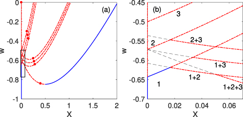
Figure 4. Critical manifold of three coupled lasers, with 23 = 8 branches. From left to right, we have the OFF-branch, three branches with one laser on, three branches with two lasers on and the ON-branch with all three lasers on. Full blue lines are attracting parts of the critical manifold, red dashdotted lines are repelling, grey dashed lines represent unphysical parts of a branch. The fixed points (all unstable) are indicated with red circles. Panel (b) magnifies the rectangular area indicated in panel (a) in which the branches emerge. The lasers that are on are indicated next to each branch. Parameters are δ1 = 1.45, δ2 = 1.4 and δ3 = 1.35.
Download figure:
Standard image High-resolution imageWe calculate the linear stability of these branches in appendix  ; at this point branch '1' emerges and the OFF-branch becomes repelling in the direction of the first laser. The other symmetrical branch, for which all lasers are 'on' (the ON-branch), is attracting for high enough intensities
  , or equivalently,
  .
.
The asymmetrical branches, with  lasers 'on', are mostly repelling: along the directions of the non-lasing nodes they are attracting only for a very small range of intensities
  . Consequently, only the branches for which
  do have a small attracting part. The point where such a branch looses stability, coincides with the emergence of a new branch, with one extra laser 'on'. Along the lasing directions, these branches are stable if
  . Combining these conditions, depending on parameters, typically only a few branches with less than half the lasers 'on', and only those with the highest thresholds δi
, have a small attracting part for low intensities.
. Combining these conditions, depending on parameters, typically only a few branches with less than half the lasers 'on', and only those with the highest thresholds δi
, have a small attracting part for low intensities.
The stability of the critical manifold for three coupled lasers is indicated in figure 4, with attracting parts in full blue lines and repelling parts in dashdotted red lines. Clearly, the two symmetrical branches, where all lasers are 'on' (ON-branch) and where all lasers are 'off' (OFF-branch), have a large attracting part. The six asymmetrical branches are mostly repelling, with only one of them (the branch with laser 1 'on') having a small attracting part for very low intensities.
4.2. Experiment: the intricate critical manifold
To uncover experimentally indications of the phase space structure described in the previous subsection, we run the experiment in the relaxation oscillations regime of the fully coupled network, where the system periodically switches between two main branches of the slow manifold, the ON branch and the OFF branch. From the theoretical analysis, one expects that this switching actually occurs through a series of steps where each laser leaves its 'off' state, the whole network going through a complex set of branches of the slow manifold. We show an example of this on figure 5.
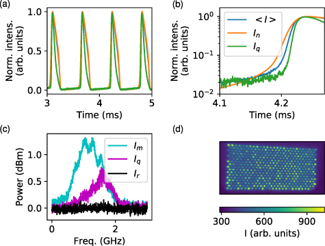
Figure 5. Experimental relaxation oscillations of the fully coupled network. Top left (a): the periodic dynamics are observed at the total intensity level (blue trace) as well as at the level of the single elements (orange and green). Top right (b): zoom over one of the switching events for the total intensity and two individual lasers. On all these traces we show the normalized laser intensity to facilitate comparison between the traces. All detectors have MHz detection bandwidth, i.e. faster than the slow time scale but slower than the two fast time scales (carriers and field). Bottom left (c): power spectra of three different lasers during the slow relaxation oscillations cycle, showing the laser relaxation oscillations (GHz frequency). Bottom right (d): still image of the array in absence of optoelectronic feedback showing the different states of each laser. The array drive DC current is 180.1 mA. At that current, when uncoupled, the network emits 2.1 mW out of which only 0.48 mW reach the feedback detector.
Download figure:
Standard image High-resolution imageThe complex structure of the critical manifold of the fully connected network cannot be observed easily at the network level especially since, as observed in section 4.1, only a small number of the 2N branches (besides the ON and OFF ones) are stable and only in a very small parameter region. However, one can still expect to observe that the network cycles among many distinct states, each one corresponding to a different number of lasers in their 'off' or 'on' states. Thus, a signature of the phase space structure can be identified by monitoring two very different nodes, as shown on figure 5(a) and (b). In this case, lasers n and q, selected for their different threshold current, leave their unstable 'off' state at different times during the periodic oscillations. However, most of the dynamics clearly takes place between the two main OFF and ON branches, where all lasers are either 'on' or 'off'.
In this oscillatory regime, the logarithmic and linear amplifiers of the feedback loop are set such that the current driving the whole network oscillates between 158.1 and 219.2 mA during the oscillation cycle, so that nearly all lasers are periodically switching 'on' and 'off'. This of course leads to exciting laser relaxation oscillations in each individual node. These correspond to the fast oscillations at the onset of the 'on' phase in figure 2 panel (b). Each laser shows a different radiofrequency power spectrum (see figure 5(c)), since all of them orbit around a different region with respect to their coherent emission threshold. The different local maxima in some peaks also exist even in the absence of optoelectronic reinjection. Their position does not appear to change under modification of any externally accessible parameter. They are therefore an intrinsic feature of the laser array, which does not seem to influence much our experimental observations beyond that. These laser relaxation oscillations (detected here by a Thorlabs PDA8GS detector with 9 GHz bandwidth) can only be observed in the power spectrum due to detection and physical noise. This observation is not unexpected when the slowest variable is orders of magnitude slower than the other two. Moreover, it clearly hints at the relevance of physical noise for a proper description of the system when each node leaves its 'off' state [70, 71].
5. Influence of noise and canard resonance
In this section, we depart from the deterministic model and analyse numerically the impact of noise on the dynamics. First we confirm the role of noise in blurring the fast laser relaxation oscillations and second we analyse the canard trajectories of individual lasers in presence of noise. Finally, we demonstrate numerically that an optimum level of noise can lead to an enhanced ordering across the network.
5.1. Noise and the canard trajectories
As underlined in section 4.2, laser relaxation oscillations can be experimentally observed only in the Fourier domain, which hints at noise causing much smaller overshoots than those presented on the numerical traces in figure 7(a) or even figure 2(b). We verify numerically at a basic level that the addition of noise in the simulations leads to a better correspondence between theoretical and experimental data: in figure 6, we show the normalized intensity of two different lasers together with the total intensity in logarithmic scale, in presence and absence of noise, mimicking the experimental figure 5.

Figure 6. Numerical timetraces of a population of N = 31 lasers in the oscillatory regime, without (resp. with) noise (a) (resp. (b)) in logarithmic scale, after applying a moving average filter (width 499) to mimic the experimental data. We show the mean intensity X (blue) and the intensities x1 (green) and x31 (orange) of the lasers with highest and lowest value of δi
. Other parameters are δ = 1.2, Δδ = 0.01,  and σ = 3 × 10⁻².
Download figure:
Standard image High-resolution image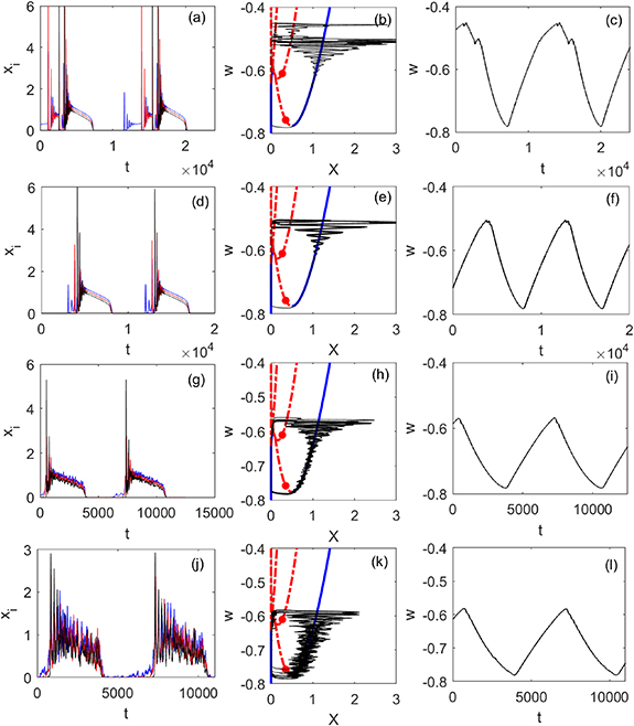
Figure 7. Left: timetrace of three coupled lasers in the oscillating regime. Middle: trajectory of the waveform in the (X, w) plane. Full lines are attracting parts of the critical manifold, dasheddotted lines are repelling. Right: timetrace of the slow parameter w(t). Parameters are δ1 = 1.45, δ2 = 1.35, δ3 = 1.25 and σ = 0 (a)–(c), σ = 10−15 (d)–(f), σ = 5 × 10⁻³ (g)–(i) and σ = 2 × 10⁻² (j)–(l).
Download figure:
Standard image High-resolution imageIn the numerical simulations without noise (figure 6(a)) the lasers switch on one by one, in order of their pump currents δi . The transition is abrupt for all lasers (but smooths out for the mean intensity), and there is a considerable time difference between the switching on of the first and the last laser. When including noise in the simulations (figure 6(b)) we see some experimental features reproduced: the first laser intensity (green) increases first in a gradual way, but the spikes are fairly simultaneous.
The above effect is to some extent not unexpected: from the phase space structure described in section 4.1 the network should leave the OFF branch via a series of asymmetrical canard branches, each laser leaving its 'off' state one after the other. Since canard orbits are known to be extremely sensitive to noise (see e.g. [72, 73]), one can expect noise to strongly influence that part of the dynamics. Beyond that however, as we shall see, noise can also have an unexpected ordering effect across this heterogeneous network. We analyse this first for a small network of three lasers by studying the departure from the OFF manifold for increasing amount of noise.
A typical time trace and phase plot in the deterministic regime is shown in figure 7(a) and (b): Starting on the OFF branch, the system follows this branch as w(t) increases. Although this branch becomes unstable as  , we find that the system stays close to it for a while longer, until, at some point, the first laser (blue curve) switches on. This constitutes a first canard. After a few laser relaxation oscillations, the system settles on the repelling branch with laser 1 'on', and the two other lasers switched off. The next laser to switch on is laser 2 (red curve), which again follows a piece of canard orbit, the system remaining close to this repelling branch corresponding to lasers 1 and 2 switched on. Then follows laser 3, and the system follows the attracting ON-branch, until it reaches
  and all lasers switch off.
This pattern, of the lasers switching on one by one, in order of the pump currents, is found for any population size and parameter set, and becomes more pronounced as the difference between the lasing thresholds δi increases. As is typical for canard dynamics, the system remains close to the branches of the slow manifold, after they have become repelling. In particular, for our choice of parameters, the system follows a repelling part of the OFF-branch, and repelling parts of the asymmetric branches. Thus, in the deterministic case, the whole process of switching from the main OFF to the main ON branches occurs via a series of canard orbits.
In the stochastic case instead, noise can drive the system away quicker from the repelling branches, towards attracting branches. Because the attracting part of the critical manifold mostly consists of the symmetric branches (ON-branch with all lasers 'on', and the OFF branch), and the asymmetric branches are mostly repelling, the coherence of the population increases with low noise. This is easily observed on figure 7: noise reduces the time the system spends on the repelling asymmetric branches, as can be seen by comparing the waveforms and phase plots without noise (panels a, b) and with low noise (panels c, d); if noise is too strong the oscillations become less coherent (panels g, h). Between the extreme values, there is an optimal noise level (panels e, f), that balances these two effects, and for which the dynamics of the population is maximally ordered.
This observation indicates that the population across the network is maximally coherent for an optimal noise level, beyond which point noise starts to dominate the dynamics.
5.2. Canard resonance
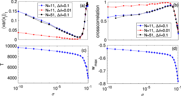
We quantify this canard resonance effect in the following two ways: First, we average the variance of the intensities of the population over time. Second, we compute the cross-correlation between the intensities of the lasers in the population with the highest and the lowest threshold, which are expected to have the two waveforms that differ most. The results are shown in figure 8 the variance, shown in panel (a), decreases logarithmically with the noise strength σ, until it reaches a resonance point around σ ≈ 4 × 10⁻³. When increasing the noise level further, the variance rapidly increases again. This resonance effect is more pronounced when the population is less homogenous and the different δi
are further apart—this is clear when comparing the variances for  (blue diamonds) and Δδ = 0.01 (red circles). The variance is minimal for slightly lower noise values in a more homogeneous population, but this effect is not large. Moreover, the population size does not seem to have much influence: the variance and correlation are almost identical in populations of 11 and 51 lasers (blue diamonds and black dots, respectively).
Figure 8. (a) Time-averaged population variance and (b) cross-correlation between the intensities of the lasers with the lowest and highest lasing thresholds x1 and xN
, for populations of size N = 11 (blue diamonds, red squares) and N = 51 (black circles) and a different spread of thresholds  (blue, black) and Δδ = 0.01 (red),
  . The mean pump threshold is δ = 1.4 in the three populations. (c) Mean period and (d) maximal amplitude
  over the timetrace for varying noise strength σ, for N = 11 and Δδ = 0.1.
Download figure:
Standard image High-resolution image
The effect is dynamical: looking at the amplitude of the oscillations of the slow variable  , and the mean period T, both decrease linearly with the logarithm of the noise strength lnσ (shown in figures 8(c) and (d)). This is an effect of so-called 'early jumps' [73] away from the repelling part of the canard solution. An intuitive explanation is that the fast variables move away exponentially slow from the repelling branch,
  , and thus, a perturbation of
  results in an approximately logarithmic decrease of both the time and distance travelled along the repelling branch (see also [71]). At resonance, the maximal amplitude point
  approaches the maximal value of w on the attracting branches (the difference is of the order of the typical variations due to noise). Thus, past the resonance point, the system no longer follows any repelling branch of the critical manifold, and is thus no longer on a canard trajectory.
Past the resonance point, we observe different scaling: both the amplitude  and the mean period T show a decrease with the noise strength σ that is closer to linear, as shown in figures 8(b) and (d). The scaling can be understood from the following analysis. Since canard trajectories have essentially disappeared in the noisy system, the switch between two branches involves leaving the still attracting OFF branch towards the attracting ON branch. Thus, the system needs to leave the basin of attraction of the OFF branch, which is determined by the stable manifold of the repelling part of the ON branch. The distance between this manifold and the ON branch is linear with w in first order, and thus the maximal jumping point
  decreases linearly with the noise strength σ.
6. Summary and conclusion
We have presented an experimental system based on an array of semiconductor lasers with optoelectronic feedback and established the excitable character of a single node. Close to five hundred nodes are coupled via their mean intensity which makes the platform interesting for the analysis of neuromorphic phenomena in large networks of slow-fast systems. The excitable dynamics is well reproduced by a phenomenological model featuring three time scales and whose dynamics can be well captured by the analysis of the critical manifold. When all lasers are coupled, the intricate structure of the critical manifold can be determined analytically and a signature of its very peculiar structure can be recognized in the experimental observations. The clear differences between some of the experimental observations and the deterministic dynamics (together with known physics of semiconductor lasers) have prompted us to introduce noise in the model. This has led to a better match between the experimental and numerical observations but more importantly, an in-depth numerical analysis of the stochastic model has brought to light several unexpected phenomena. First, in spite of the fact that the collective dynamics of the system cannot be reduced to a simple ordinary differential equation when the number of nodes tends to infinity, we show that noise can in fact simplify the dynamics of the network by enhancing the coherence of the canard trajectories at the onset of lasing. In some sense, noise helps in reducing the complexity of the dynamics of the network towards that of a simple low dimensional system. Second, we have identified numerically a new phenomenon that we have named 'canard resonance', whereby the ordering of the different trajectories followed by each node of the network displays a maximum for a non vanishing amount of noise. Numerical observations indicate that the most ordered state could also be reached by tuning ε but this parameter can not be tuned over a very wide range in this experimental implementation. Although the matching experimental observation is not possible in the current set up, it is not unrealistic to envision an experimental realization of canard resonance in an evolution of the present set up (essentially making the experimental time scale separation smaller) or in other slow-fast optical or biological platforms. Besides this, further directions of work which may be envisioned on the current experimental platform include the analysis of excitability at the network level and the coupling of networks of networks.
Acknowledgments
O D has received funding from the European Union's Horizon 2020 research and innovation programme under the Marie Sklodowska-Curie Grant Agreement No. 713694.
Appendix A.: Linear stability of the critical manifold
The stability of a branch with lasers  on and lasers
  lasers off, is given by the eigenvalues of the Jacobian,
with
and
The 'off'-lasers decouple, and it is immediately clear that a branch with laser n off, is only stable if the eigenvalues of  are negative. This leads to the stability criterion along the non-lasing directions
 ![$y_i = \delta_i+k\left[w+A\ln(1+\alpha X)\right]\lt1$](https://content.cld.iop.org/journals/2515-7647/3/2/024010/revision3/jpphotonabcbe3ieqn58.gif) . Using equation (7), this leads to the criterion
. Using equation (7), this leads to the criterion  .
.
The ON-branches do not decouple. However, if all lasers with nonzero intensity are identical, one finds a Jacobian Jm
along the mean field  ,
, 
which is stable if
Transverse to the mean field, one finds a transverse Jacobian Jt (with multiplicity N+−1)
which is always stable.
In order to calculate the stability of the ON-branches for non-identical lasers, we calculate the determinant of the Jacobian restricted to the lasing elements; one finds ![$\Delta = - \gamma^{N^+}\Pi_i x_i \left[\frac{N^+ kA\alpha}{N(1+\alpha X}-1)\right]$](https://content.cld.iop.org/journals/2515-7647/3/2/024010/revision3/jpphotonabcbe3ieqn62.gif) . Given that the determinant is the product of the eigenvalues, we find that the location of the bifurcation does not change. Assuming that the eigenvalues change relative to
. Given that the determinant is the product of the eigenvalues, we find that the location of the bifurcation does not change. Assuming that the eigenvalues change relative to  , we can exclude additional bifurcations for lasers that are similar enough.