Machine learning for neutron reflectometry data analysis of two-layer thin films^*

The thin film structure used in this study is a two-layer system on a silicon substrate. The beam is incident onto the surface of the thin film layer furthest from the silicon substrate through air. Such a system can be modeled by defining an SLD profile parametrized by a stack of thin film layers, each with a thickness, an SLD, and a roughness parameter that describes the interface between two consecutive layers. Describing the SLD profile of a two-layer thin film therefore requires seven parameters (thickness, SLD, and roughness for each layer, and a substrate roughness).

Several reflectometry packages are available for creating a set of data for training a neural network [11–14]. Here, the reflectivity model calculations were done using the Refl1D package [11]. Reflectivity calculations with Refl1D use the thin film layer parameters outlined above to establish a multi-layer structure from which R(Q) is calculated. R(Q) is computed using the method of Abelès [15], where the roughness is accounted for using the approach of Névot and Croce [16]. A Q resolution of ΔQ/Q = 2.5% was used to generate the training data, a value that is consistent with the Magnetism Reflectometer [10].

The neural network developed was applied to data sets measured at the Magnetism Reflectometer [10]. The sample was a thin film of Haynes 230 nickel alloy deposited on a silicon substrate and annealed at 600^∘C, which produced a well defined two-layer structure, with a thick oxide layer on top of a nickel rich alloy layer. Nickel is a ferromagnetic material that exhibits magnetic properties when present in a high enough density. Discussion of the properties of this material [17–19] is outside the scope of this paper. This data set was selected because it provides a demonstration of the utility of the neural network and because it was possible to model it with only two thin film layers using standard methods.

The sample was measured using polarized neutron reflectometry (PNR), performed in a 1 T magnetic field in the plane of the film. PNR follows the same formalism outlined above, but leverages the neutron's magnetic moment to extract information about the magnetic structure of a thin film [20]. In this case, the SLD can be expressed as the sum of a nuclear and a magnetic component $\beta(z) = \beta_N (z) \pm \beta_M (z)$, where β_N (z) corresponds to the nuclear component, and β_M (z) corresponds to the magnetic component. The magnetic contribution to the SLD depends on the spin state of the neutron, and the + and − signs indicate spin states parallel and anti-parallel to the in-plane magnetization, respectively. The reflectivity profile was obtained for each of the two spin states and our neural network was applied to each data set independently. Using a PNR measurement to test our approach provides a use case where two distinct data sets come from the same nuclear structure, so that we expect two closely related predictions.

A neural network was used to map a theoretical SLD profile to its corresponding reflectivity curve R(Q). The intention was to train a neural network to predict the seven thin film parameters corresponding to an input reflectivity curve. Given the complexity of the inverse problem of finding the underlying structure that best represents a measured scattering curve, establishing a relationship between a given theoretical R(Q) curve and physically plausible SLD profile is particularly valuable. Focusing on mapping the theoretical R(Q) to the underlying SLD profile also has the advantage of only necessitating simulated data. The approach allows for a diverse range of model parameters, and makes it possible to employ a larger training set than would be possible if real, measured data were to be used. This approach also intentionally separates the challenge of mapping a given theoretical reflectivity curve to its underlying SLD profile from understanding the impact of statistical fluctuations in measured data on the predictions.

For each thin film model, all thin film layer parameters were generated using a uniform random distribution from within a predefined range (see supplemental table S1 (available online at stacks.iop.org/MLST/2/035001/mmedia)). To ensure good predictions, the choice of the range of each parameter should be selected to cover all measurable values. The range of each parameter in the model was selected to produce a reasonable distribution of model structures that could be studied with a neutron reflectometer instrument. The neural network, described below, was constructed such that each neuron of the input layer corresponded to a reflectivity value for a given point in Q. Therefore, a common array of Q values was used in evaluating R(Q), and the experimental data was measured at the same Q values to avoid potential errors due to interpolation. In the present study, the Q array had 92 points in the range $0.008 \lt Q \lt 0.088$ Å⁻¹. The training set consisted of reflectivity curves calculated from one million randomly generated thin film structures, of which the last 10 000 were used as a validation set for the training.

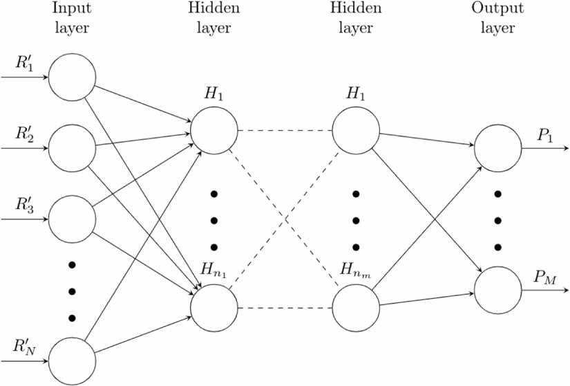
A neural network with six hidden layers was used to model our reflectometry data using TensorFlow [21]. The neural network is shown schematically in figure 1. The input layer consisted of a number of neurons equal to the number of Q values at which the reflectivity profile was measured. The performance of neural networks improves when the input parameters vary within a limited range of values [22]. Reflectivity profiles, on the other hand, can span up to 6 or 7 orders of magnitude. For this reason, the input R(Q) profiles were preprocessed before being used as the input layer to our neural network. For a given R(Q), the following function was applied:

$$\begin{equation} R^{\prime}(Q) = \log\left[\frac{Q^2}{Q_0^2} R(Q)\right], \end{equation} \tag{ 3 }$$

where $R^{^{\prime}}(Q)$ is passed to the input layer of the neural network and Q₀ is the value of the first Q value. The inclusion of Q₀ has no effect on the neural network and was only added for convenience to keep a reasonable scale. The same preprocessing was applied to real data when predicting thin film parameters with the neural network. It should be noted from equation (1) that choosing a multiplicative factor of Q⁴ may further minimize the amplitude range of R(Q). On the other hand, the uncertainty on a real measurement tends to increase with Q as the counting statistics get poorer. A reasonable approximation of the dependence of the uncertainty on Q in a real reflectivity measurement is to assume simple counting statistics, which leads to $\Delta R/R \propto \sqrt{R}/R \propto Q^2$. Knowing that the ultimate goal is to test our neural network with real measurements, a good preprocessing scheme for R(Q) should serve both the purpose of enabling efficient training and stabilizing predictions. Our choice for the preprocessing of the R(Q) values passed to the input layer was also chosen with the cost function used for training in mind. The cost function used was the mean squared error (MSE), defined as

$$\begin{equation} {\text{MSE}} = 1/N \sum_{i = 1}^N (R^{^{\prime}}_i-R^{\prime{\text{pred}}}_i)^2, \end{equation} \tag{ 4 }$$

where the sum runs over every Q point, $R^{^{\prime}}_i$ is the preprocessed reflectivity value at the ith point, and $R^{\prime{{pred}}}_i$ is the predicted value of $R^{^{\prime}}(Q)$ at that point. Our choice of $R^{^{\prime}}(Q)$ therefore uses a factor proportional to the uncertainty on each point to give more weight to points at lower Q where the relative uncertainty is smallest.

Zoom In Zoom Out Reset image size

The number of hidden layers and the number of neurons per layer were chosen empirically. We started with a single hidden layer and incrementally added layers until we could obtain a qualitatively reasonable correlation between generated and predicted parameters. Since the quality of the predictions also depends on the size of the training set and the number of epochs chosen to train the neural network, these were selected using the same approach. After exploration, we determined that six hidden layers worked well for the problem. The number of neurons was 300 for the first hidden layer, 400 for the second, third and fourth hidden layers and 100 and 50 for the fifth and sixth hidden layers, respectively.

The output layer of the neural network consisted of the seven structural parameters needed to describe the two-layer structure on silicon. The thin film structure parameters themselves were normalized to [−1, 1] within their respective value range. The predictions were then transformed to the original ranges that the neural network was trained with.

The Adam optimizer [23] was used to train the neural network, with a learning rate parameter of 5 × 10⁻⁴. The scaled exponential linear unit activation function was used [24] along with the LeCun kernel initializer [25]. Figure 2 shows the loss function value as a function of epoch, as well as the loss function value for the validation set. The neural network model was trained for 20 epochs. The number of epochs was chosen such that the loss function value (see equation (4)) of the validation set remained similar to the loss function value of the training set. Above 20 epochs, the loss for the training set was more likely to dip below the loss for the validation set, indicating the possibility of over-fitting. The code that was used to generate the training set and train the neural network is available on GitHub [26], along with the trained network.

Zoom In Zoom Out Reset image size

To evaluate how well the trained neural network performed, we generated 100 000 new thin film models using the same procedure used to develop the training set. For each R(Q) in this set, the seven parameter predictions were generated by querying the neural network. Figure 3 shows how well the neural network predictions matched the generated parameters. Each sub-figure in figure 3 was obtained by histogramming the 100 000 pairs of predicted and generated parameters. Supplemental figure S1 shows the deviation of each predicted parameter, $\Delta P = P_{\textrm{pred}} - P_{\textrm{true}}$, for the same data. All thin film model parameters are very well modeled. The predictions for the SLD of the bottom layer (SLD$_{\textrm{bot}}$) close the SLD of silicon (2.07 × 10⁻⁶ Å⁻²) are not as well reproduced. This outcome is to be expected, since in this case the bottom layer blends in with the substrate. Very low roughness values are slightly less well reproduced. This is to be expected, as low roughness values will have a smaller effect on the reflectivity profile compared to larger roughness values. It should be pointed out that predictions can also be distorted near the edges of the chosen parameter ranges. This can be seen on several sub-figures of figure 3, but especially for the roughness parameters. Although inevitable in the case of a physical limit, this highlights the need to select a training set having parameter ranges with wide enough margins to minimize distortions when the neural network is used for a particular application. Supplemental figure S2 shows an example of how the choice of the range of $\sigma_{\textrm{bot}}$ affects the predictions.

Zoom In Zoom Out Reset image size

Our neural network was trained on reflectivity profiles without statistical variations on each R(Q) point, yet real experimental data always have them. The loss of phase information intrinsic to reflectometry measurements makes reflectivity modeling a challenging endeavor and is compounded by the statistical variations in measured data. Therefore, it is vital that a neural network should be able to make predictions that are stable with input data that possess statistical fluctuations that are representative of those encountered in real measurements. A usable neural network needs to map that solution space well enough to offer stable predictions. This requirement is particularly important because of the 'black box' aspect of neural networks that parametrize a solution space in a way that does not lend itself to a simple interpretation. In this section, we investigate the effect of counting statistics on the neural network predictions.

To simulate measurement statistics, we generated 100 000 new reflectivity profiles using the approach described in section 2.3. For each profile, statistical fluctuations were added to each R(Q_i ) point by adding a random value δR(Q_i ) selected from a Gaussian distribution with a standard deviation $\sigma_{R_i}$. In order to simulate realistic fluctuations, the standard deviation for each point i was set to $\sigma_{R_i} = (\Delta R_i/R_i)_{\textrm{meas}} \times R(Q_i)$, where $(\Delta R_i/R_i)_{\textrm{meas}}$ corresponds to the relative uncertainty on the ith point in Q of one of the two measurements performed at the Magnetism Reflectometer and described in section 2.2 (for this purpose, both measurements have similar uncertainties and would be equally suitable. We chose the spin-down measurement). Following the generation of this new data set, our trained neural network was used to predict thin film structure parameters for each of the 100 000 simulated measurements.

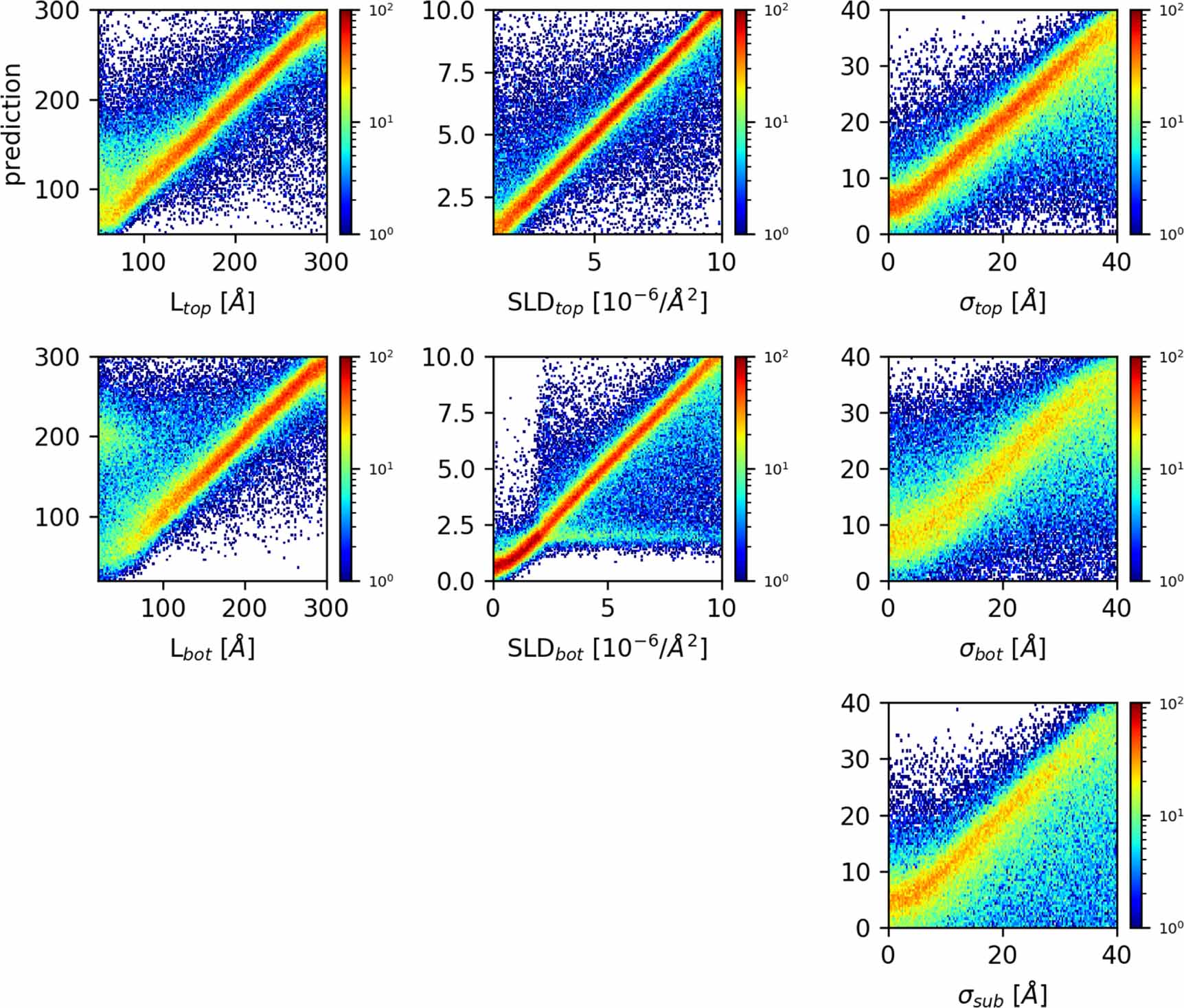
Figure 4 shows the relationship between the predicted and true values for each of the seven parameters. Supplemental figure S3 shows the distribution of the deviation $\Delta P = P_{\textrm{pred}} - P_{\textrm{true}}$ for each parameter. Similar to the case without statistical fluctuations, most parameters are well modeled by the neural network. The roughness parameters $\sigma_{\textrm{sub}}$ between the substrate and the bottom layer, and $\sigma_{\textrm{bot}}$ between the bottom and top layers are not as well modeled and show a tail toward smaller values. This result is not surprising. These two roughness parameters mainly affect the high-Q tail of the reflectivity curve, where the measurement uncertainties are larger. Although statistical fluctuations of the measurements will translate in a wider range of predictions for roughness parameters, they do not prevent the neural network from providing valuable structure predictions. The L$_{\textrm{bot}}$ values below 50 Å are not well reproduced. In particular, predictions for simulated data with true L$_{\textrm{bot}}$ values below 50 Å can be very large, as can be seen on figure 4. Investigating those simulations, we found that they mostly corresponded to thin film structures with large values of SLD$_{\textrm{top}}\gt6\times 10^{-6}$ Å⁻² where the SLD profile of the film could be interpreted as a single layer. For these simulations, the neural network still interprets the data as a two-layer system, with a larger L$_{\textrm{bot}}$ than its true value.

Zoom In Zoom Out Reset image size

A clear difference can be seen in the quality of the predictions for SLD$_{\textrm{bot}}$ values below the SLD of silicon compared to higher SLD$_{\textrm{bot}}$ values. Statistical fluctuations have a smaller effect for SLD$_{\textrm{bot}}\lt2\times 10^{-6}$ Å⁻² where a critical edge is more likely to be visible. Our analysis demonstrates that a neural network can be used to map a reflectivity curve R(Q) to an estimate of its underlying SLD profile within reasonable uncertainty.

The trained neural network model was applied to PNR data collected from the Haynes 230 sample described in section 2.2, which was obtained with the Magnetism Reflectometer [10] at ORNL. The measured reflectivity R(Q) was binned to the Q binning chosen to train our neural network, and each measurement was preprocessed using equation (3) to obtain $R^{^{\prime}}(Q)$.

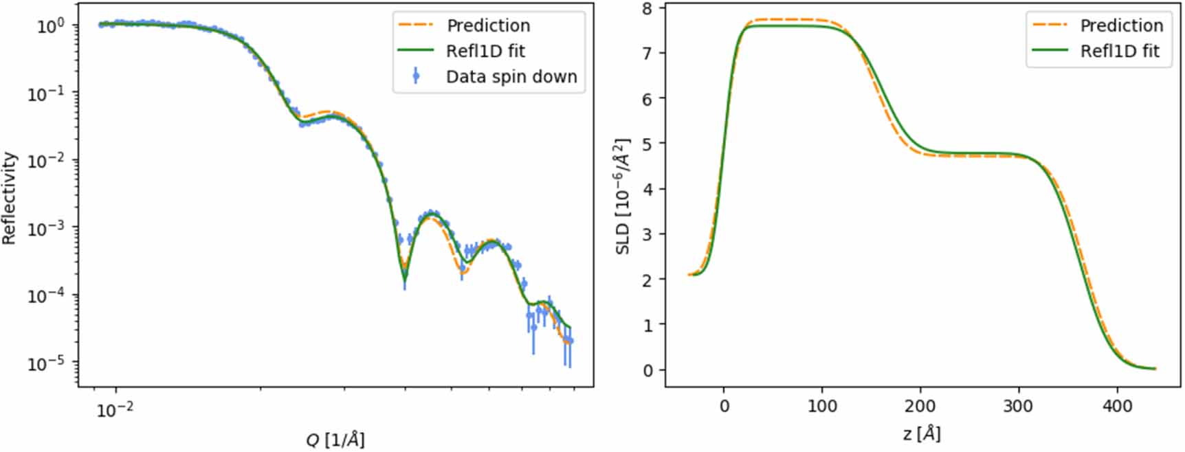
The left panel of figures 5 and 6 show the measured reflectivity profiles and the neural network predictions for the two measured neutron spin states. The predictions are compared with fit results obtained using the Refl1D software using the DREAM algorithm [27] for the minimization process. Since the nuclear structure is the same for both measured spin states, these were fit simultaneously using the same thin film structure. All parameters were constrained to be the same for both data sets, except for the SLD of the magnetic bottom layer which was let to vary with each data set. Setting up the constrained fit was done using the Webi reflectometry application developed at ORNL [28]. The fit parameters are shown in table 1 and compared with the prediction for each spin state. The right panel of figures 5 and 6 show the comparison between the fitted model and the neural network predictions. Both the predicted SLD profiles and the corresponding reflectivity curves agree well with the fit results.

Zoom In Zoom Out Reset image size

Zoom In Zoom Out Reset image size

Table 1. Fit results for the Haynes 230 data, compared with the neural network predictions. The uncertainties in the fit results column refer to the Bayesian probability density function for each parameter given the measured data. The standard deviations in the NN prediction column refer to the probability density function of the prediction for repeated measurements of a particular thin film.

	Spin down		Spin up
Parameter	NN prediction	Fit result	NN prediction	Fit result
L${}_{\textrm{top}}$ (Å)	212 ± 11	200.3 ± 1.3	202 ± 18	200.3 ± 1.3
SLD${}_{\textrm{top}}$ ($10^{-6}~{\unicode{x00C5}}^{-2}$)	4.89 ± 0.36	4.77 ± 0.04	4.96 ± 0.43	4.77 ± 0.04
$\sigma_{\textrm{top}}$ (Å)	23.3 ± 2.8	25.3 ± 0.9	20.7 ± 4.0	25.3 ± 0.9
L${}_{\textrm{bot}}$ (Å)	157 ± 10	161.4 ± 1.2	167 ± 20	161.4 ± 1.2
SLD${}_{\textrm{bot}}$ ($10^{-6}~{\unicode{x00C5}}^{-2}$)	7.66 ± 0.33	7.58 ± 0.03	6.63 ± 0.42	6.80 ± 0.02
$\sigma_{\textrm{bot}}$ (Å)	19.3 ± 4.0	23.6 ± 1.6	15.7 ± 6.1	23.6 ± 1.6
$\sigma_{\textrm{sub}}$ (Å)	13.6 ± 2.4	9.9 ± 0.5	13.3 ± 3.9	9.9 ± 0.5
χ2	5.0	1.2	3.8	1.0

To expand our understanding of the stability of the neural network predictions to statistical fluctuations, the technique used in the previous section was applied to the measured data. Each point of the measured R(Q) data set was randomly varied according to a Gaussian distribution with a standard deviation equal to the measurement uncertainty of each point. This process was used to generate a new set of 20 000 simulated measurements and the neural network was then used to predict thin film parameters from these 20 000 simulated R(Q) profiles. The distribution of the predicted values for each parameter is shown in supplemental figures S4 and S5. The standard deviation of the distribution of predictions for each parameter was used to estimate the stability of the prediction for that parameter, and are quoted as the uncertainty of the neural network predictions in table 1. The predicted parameters agree well with the fit results for both measured data sets, which demonstrates the feasibility of using a neural network to obtain a thin film structure prediction for a reflectivity measurement. Such predictions could readily be used in subsequent automated processes, or could be used as an initial model for traditional data fitting.

The standard deviation values quoted in table 1 with the network predictions have a different meaning than the parameter uncertainties produced by the DREAM algorithm [27] implemented in Refl1D [11]. The Refl1D package uses a Bayesian approach to determine the uncertainty on model parameters. The results are meant to be interpreted as a probability density function for each parameter given the measured data. In our case, once our neural network is trained, each input reflectivity curve has a single well-defined neural network output. For a particular underlying (true) thin film structure, the probability of observing a given reflectivity profile given statistical fluctuations is also the probability of obtaining the corresponding neural network prediction. The standard deviation on each parameter prediction in table 1 is an estimate of the expected variations in the prediction of each thin film parameter one would obtain if this particular measurement were repeated a larger number of times. The fact that the standard deviation of each parameter prediction is larger than the uncertainty of the corresponding fit parameter demonstrates the importance of follow-on refinement fitting for final data analysis.