

Abstract
An electron-cyclotron resonance thruster (ECRT) prototype is simulated numerically, using two coupled models: a hybrid particle-in-cell/fluid model for the integration of the plasma transport and a frequency-domain full-wave finite-element model for the computation of the fast electromagnetic (EM) fields. The quasi-stationary plasma response, fast EM fields, power deposition, particle and energy fluxes to the walls, and thruster performance figures at the nominal operating point are discussed, showing good agreement with the available experimental data. The ECRT plasma discharge contains multiple EM field propagation/evanescence regimes that depend on the plasma density and applied magnetic field that determine the flow and absorption of power in the device. The power absorption is found to be mainly driven by radial fast electric fields at the electron-cyclotron resonance region, and specifically close to the inner rod. Large cross-field electron temperature gradients are observed, with maxima close to the inner rod. This, in turn, results in large localized particle and energy fluxes to this component.
Export citation and abstract BibTeX RIS
1. Introduction
The electron cyclotron resonance thruster (ECRT) [1–6] belongs to the category of electrodeless plasma thrusters. Another example of this family of devices is the helicon plasma thruster (HPT) [7, 8]. These thrusters use electromagnetic (EM) heating to generate and energize the plasma, and thus allow eliminating exposed electrodes from their design, which are often lifetime-limiting components. The ECRT relies on the localized absorption of EM power at an electron-cyclotron resonance (ECR) region, whereas the HPT is based on non-resonant heating. Both concepts utilize a cylindrical ionization source and an external magnetic nozzle (MN) to expand the plasma contactlessly and create magnetic thrust. The ECRT, which is the object of the present work, should not be mistaken with the gridded ion thrusters based on ECR heating [9].
The first investigation of this propulsion concept began in 1962 [1], using a waveguide to deliver the power into a cylindrical discharge chamber with an externally-applied magnetic field that ensured resonance conditions and configured the external MN. In [2], a 2% efficiency thruster with 22% energy and 80%–90% coupling efficiencies were reported for a 320 W argon prototype without performing any optimization of the device. In [3, 4], devices up to 15% thrust efficiency were built and tested. Similar performance was obtained recently as well [10–18].
A successful model of the ECRT must take into account the plasma transport problem and the plasma-wave problem, which are intimately coupled together. Existing ECRT transport models are (quasi) one-dimensional and either take a fluid quasineutral approach [6] or a particle-in-cell (PIC) approach [19]. More recent models focus on the HPT [20–22], but these models are in general applicable for the ECRT as these two thrusters share most characteristics in terms of transport phenomena.
On the other hand, plasma-wave interaction models in ECR plasmas have different requirements than those used for the HPT [23, 24] due to the presence of a resonance and highly inhomogeneous EM properties. Models for ECR heating have been developed for other applications as for fusion tokamaks [25, 26], ECR ion source plasmas [27] or plasma etching [28]. The physical phenomena governing plasma-wave interaction, wave propagation and absorption in ECR plasmas have been investigated in the past [29–33], mainly with 1D models. Methods used for wave simulation as beam/ray tracing algorithms [34, 35], while useful to obtain a first insight on propagation and absorption characteristics, are not adequate for an accurate assessment of the ECRT since the device characteristic length is comparable to the wavelength. A full-wave approach, that obtains solutions of Maxwell's equations directly in the simulation, either in time domain [36, 37] or frequency domain [38, 39], becomes necessary.
Despite these advances, the simultaneous and self-consistent computation of the plasma transport and the fast EM fields in the ECRT has not been achieved so far. As the power deposition can affect the plasma response and vice versa, this coupling becomes necessary to understand the physics and the operation of the device and properly estimate its performance. Indeed, existing comparisons between experimental and theoretical results [6] of an argon tested device report large differences between the measured and expected, jet efficiency (e.g. 41% compared to a 2%) and coupling efficiency (e.g. 98% compared to a 30%). Further contemporary comparisons for the ECRT [14] accomplished a fairer agreement between measurements and theoretical estimations using an HPT model [22]. However, that model not only underestimates the steady-state electron temperature, but also does not describe the plasma cross-field diffusion and antenna/plasma power coupling. As a result, that model cannot reproduce radial profiles in plasma density, nor the power transfer efficiencies.
Recently, the European H2020 MINOTOR project [40] was funded to investigate and continue the development of the ECRT concept, with the purpose of demonstrating its feasibility for space propulsion. In the context of this project, a two-dimensional, axisymmetric model of the ECRT discharge has been developed to enable parametric investigations of the operation of this device, both to improve the current understanding of the complex phenomena within the thruster as well as to support the development of the prototype. The model is composed of two main components which are coupled together to obtain the plasma and EM field response in the thruster: (i) a hybrid PIC/fluid model to solve for the internal and near-plume plasma transport, and (ii) a full-wave, finite element (FE) model of the EM field-plasma problem in the frequency domain to solve the EM fields and the power absorption in the device. An initial version of the former has been reported independently in [41–44], while the latter was introduced in [45, 46].
In this work, we use this approach to simulate numerically the ECRT prototype developed by ONERA as part of the MINOTOR project in its nominal operating point [16–18], solving the coupled plasma transport problem and the EM problem. The maps of the different plasma properties and EM fields are discussed, together with the particle and energy wall fluxes. Finally, the performance parameters of the thruster are compared against the available experimental data, to provide a partial validation of the model.
The rest of the paper is structured as follows. The physical and numerical models used in each module and the simulation setup are described in section 2. Section 3 presents and discusses the simulation results. Finally, conclusions and future work are listed in section 4. Appendices
2. Simulation model
The design of an ECRT (see figure 1) consists of a rear wall and a cylindrical lateral wall that form the thruster chamber. The chamber contains an inner rod element along its centerline. All these elements are metallic and covered by a thin boron nitride coating. Neutral xenon gas is fed into the chamber through injector holes on the rear wall. A coaxial cable feeds EM power to the thruster through a dielectric window located at the center of the rear wall. The core conductor of the coaxial cable is electrically connected to the metal of the inner rod element, and the shield of the coaxial cable is electrically connected to the metal of the rear and lateral walls. A divergent applied magnetic field creates a MN that is used to accelerate the plasma as shown in figure 1 and sets up the conditions for the ECR inside the thruster chamber.

Figure 1. Sketch of the ECRT simulation domain. For geometrical dimensions refer to table 1. The arc-length variable ζ covers the perimeter of the thruster wall meridian section.
Download figure:
Standard image High-resolution imageThe model and code presented here have been tailored for the simulation of this coaxial ECRT, but are applicable to more general thruster types. The overall structure of the simulation model is shown in figure 2, and is based on the separation of two distinct time scales: that of the slow (up to a few MHz) plasma transport response, and that of the fast (GHz) applied EM field. The model is composed of three main modules: (i) the so-called ion (I-) module, solving the slow response of the heavy species (i.e. ions and neutrals). (ii) The electron (E-) module, solving the slow response of the electrons and the quasineutral, quasi-stationary electric potential map. The E-module also takes care of solving the thin non-neutral Debye sheaths that form on the (dielectric) thruster walls, the secondary electron emission (SEE), and the particle and energy fluxes to the walls. (iii) The wave (W-) module, solving the fast time scale interaction between the EM emission and the electrons. The I- and E-modules describe the quasi-stationary transport of the plasma. The features of these two modules have been described in references [41–44, 46–48]. Their main aspects are described briefly in the next subsections. The W-module [45, 46] is a new development and is thus described in detail afterwards; its numerical verification is presented in appendix
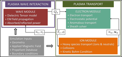
Figure 2. Overall code structure, composed of an ion/neutral module, an electron module, and a wave module.
Download figure:
Standard image High-resolution imageSymbols E and B are reserved for the high frequency EM fields. The static magnetic field applied by the coils is called B 0, and the quasi-steady electric field is denoted as −∇ϕ, with ϕ the electrostatic potential. Symbols ns , Ts , u s , j s , refer to the quasi-steady density, temperature, macroscopic velocity and current density, respectively, of a generic plasma species s. The right-handed cylindrical vector basis, {1z , 1r , 1θ }, and the unit vectors 1∥ = B 0/B0, 1⊥ = 1θ × 1∥, and 1n (outward unitary normal vector at the domain boundary) are used in the following. Without loss of generality, we take B 0 pointing downstream.
As explained in more detail later, the four modules are run sequentially, in close loop, with different timesteps, communicating with each other to share the relevant variables. In particular, the E-module takes as inputs nα and u α of all heavy species α from the I-module, and delivers ϕ and Te to that module. In addition, the E-module takes the time-averaged absorbed power density Qa as input from the W-module and delivers ne and the electron total collision frequency νe to that module. Each module utilizes a different grid or mesh, optimized for its own requirements, and interpolation between the meshes is applied. The simulation domain for the I- and E-modules (in red in figure 1) consists of the thruster chamber and the MN region. The simulation domain for the W-module (in black in figure 1) adds a segment of the coaxial power feed cable.
2.1. The I-module
For the heavy species, a PIC formulation with Monte Carlo collisions is used [41]. Macroparticles evolve in a structured mesh subject to (i) a particle mover that propagates the trajectory of the macroparticles with a leap-flog scheme subject to the quasi-steady fields −∇ϕ and
B
0; (ii) various types of collisions, including ionization (e.g. single, double, and single to double) by electron bombardment and charge-exchange collisions among neutrals and ions [49], (iii) the interaction with the different channel walls and their Debye sheaths, which includes neutral accommodation at the walls and re-emission, ion recombination and re-emission as neutrals, and the fulfilment of the Bohm criterion at the sheath edge [50]. At the position of the injector, a prescribed mass flow rate  of neutrals is injected into the domain. Heavy particles reaching the downstream open boundary are removed. Neutrals, singly-charged, and doubly-charged ions are treated as different heavy species and the corresponding macroparticles are kept in different computational lists, which are used for weighting their macroscopic properties onto the PIC mesh. Figure 3(a) plots the structured cylindrical-type mesh used in the I-module. The mesh is finer close to the walls to improve the characterization of gradients in the vicinity of walls. An statistical population control mechanism is implemented to each species looking for an optimal number and size of macroparticles in each cell [51]. A typical number of macroparticles per cell for this type of simulations is around 300. In order to improve the population control in the plume, the mesh cell-size is increased downstream.
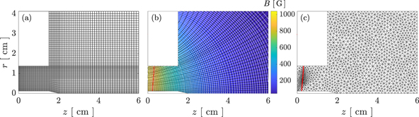
Figure 3. (a) PIC mesh, (b) MFAM and (c) representation of the W-module mesh. In (b), the colormap represents the applied magnetic field strength, magnetic streamlines are shown in black and their perpendicular in white. The red curve represents the ECR location.
Download figure:
Standard image High-resolution image2.2. The E-module
In their low-frequency response, electrons are treated as a magnetized diffusive fluid [47]. The set of fluid equations is the following:


Equation (1) states the conservation of electric current, with j i = ∑s≠e Zs ens u s the total positive current provided by the I-module. Equation (2) is the momentum equation, where electron inertia has been neglected; pe = ne Te is the (isotropic) electron pressure; and F coll = −me ne∑s≠e νes ( u e − u s ) is the resistive force due to collisions, with νes = νes (Te) the effective collision frequency of electrons at temperature Te with species s, which includes ionization and excitation collisions and elastic electron collisions with neutrals and ions.
Finally, the term F turb = 1θ αt jθe B0 in equation (2) is a phenomenological turbulence model, with αt an empirical parameter adjusted to match experimental results. Turbulence is believed to be the main source of anomalous transport in Hall thrusters, and this model (which results in a net enhancement of the electron transport perpendicular to the magnetic field) has been used successfully in the past to explain experimental measurements [52, 53]. Evidence of turbulence on electrodeless plasma thrusters like the ECRT is still very limited, but existing results [54] indicate that it is a pervasive element of these devices (and HPTs) as well. As the ECRT also features an E × B plasma like Hall thrusters, the same model is used here to introduce the effect of turbulent transport in the simulation. After a sensitivity analysis on αt, which showed it affects substantially the peak electron temperature, but little the propulsive performance figures (such as thrust and specific impulse), a value αt = 0.02 was found to match well the experimentally available Te measurements at the axis downstream [55].
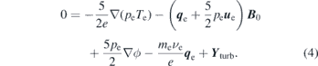
Equation (3) is the internal energy equation, where: q e is the electron heat flux; Qcoll = −ne ∑s≠e νes ɛes , (with ɛes the energy yield of the collision) is the power sink due to collisions with heavy species, mainly ionization and excitation of neutrals. Equation (4) is a diffusive model for the electron heat flux, structurally similar to the momentum equation, with νe = ∑s≠e νes , and Y turb = −1θ αt qθe B0 a turbulence-based contribution, here enhancing the perpendicular heat flux. Additionally, the quasineutrality condition

is imposed in the bulk of the simulation domain, i.e., except in the sheaths. In this expression, the right-hand side is the positive charge density, provided by the I-module, with Zs the charge number of each species.
Boundary conditions for the electron fluid equations depend on the type of surfaces. On the axis, symmetry conditions are imposed, implying that the radial electric current and electron heat flux are zero. On the current-free downstream boundaries, the net normal electric current, jn = j ⋅ 1n, is set to zero and the normal electron heat flux satisfies qne = q e ⋅ 1n = 2Te ne une. At the thruster walls the normal electric current density jn and the normal heat flux qne are computed by the sheath solver described next.
The Sheath solver relates the electron magnitudes at the sheath edge and the thruster wall. In the thruster simulated here, walls are covered by boron nitride, which has a high SEE yield, defined as the ratio of secondary-to-primary electron fluxes. The macroscopic SEE yield, δw(Te) is modelled according to reference [56], which is based on the following parameters:

where δws(Te) and δwr(Te) are yields for, respectively, (true) secondary electrons (emitted with a small temperature Tse), and elastically reflected primary electrons. For high electron temperatures δws is limited to a maximum of 0.983, when charge saturation is expected to happen [57]. The energies Es and Er are δr0 are material dependent. Additionally, the sheath model takes into account the partial depletion of the high-energy tail of primary electrons lost into the walls, with the replenishment parameter σ (equal to 100% for full replenishment). The net normal electric current to the dielectric wall, jn, with contributions of ions and primary and secondary electrons, is zero. As a result the sheath local potential fall between sheath edge Q and (dielectric) wall W, fulfills the relation

The normal heat flux to the wall, qne, is the difference of the normal flux of total electron energy, adding the contributions of primary and secondary electrons, minus the normal flux of convective energy of the electron fluid [56]. Settings here are for boron nitride: Es = 50 eV, Er = 40 eV, δr0 = 0.4, Tse = 2 eV and σ = 0.3 [52, 56, 58].
In order to avoid numerical diffusion caused by the large magnetic anisotropy, the electron fluid equations are solved in the magnetically-aligned mesh plotted in figure 3(b). Specific numerical algorithms have been developed for this [47]. For the conservation laws (1) and (3), these are based on finite volume schemes. For equations (2) and (4), which are actually state equations relating j e and q e with ϕ and Te gradients respectively, the algorithms are based on finite difference schemes. Irregular cells, next to boundaries require special attention for their accurate solution.
2.3. The W-module
The W-wave module is an axisymmetric, frequency-domain full-wave model. This model takes as inputs the maps of electron density ne and collisionality νe from the E-module. As outputs, it returns the high-frequency EM fields ![$\boldsymbol{E}\left(z,r,\theta ,t\right)=\mathfrak{R}\left[\hat{\boldsymbol{E}}\left(z,r,\theta \right)\mathrm{exp}\left(-\mathrm{i}\omega t\right)\right]$](https://content.cld.iop.org/journals/0963-0252/30/4/045005/revision3/psstabde20ieqn2.gif) ,
, ![$\boldsymbol{B}\left(z,r,\theta ,t\right)=\mathfrak{R}\left[\hat{\boldsymbol{B}}\left(z,r,\theta \right)\mathrm{exp}\left(-\mathrm{i}\omega t\right)\right]$](https://content.cld.iop.org/journals/0963-0252/30/4/045005/revision3/psstabde20ieqn3.gif) , where variables with hat are the complex field amplitudes. From these fields, the map of power absorption density, Qa, is then computed.
, where variables with hat are the complex field amplitudes. From these fields, the map of power absorption density, Qa, is then computed.
The frequency-domain of Faraday and Ampère–Maxwell's laws determine the complex amplitudes of the fields:


where μ0 is the magnetic permeability of free space, and  and
and  represent the complex amplitudes of the excitation current and the electric displacement field, respectively. Note that
  and
and  automatically satisfy
  and
and  .
.
The field  includes the contribution of vacuum permittivity and the susceptibility of the plasma. A cold plasma model is used to relate
  linearly to
  ,
,

where ɛ0 is the permittivity of free space and  is the dielectric tensor, given in the {1z
, 1r
, 1θ
} vector basis by
is the dielectric tensor, given in the {1z
, 1r
, 1θ
} vector basis by
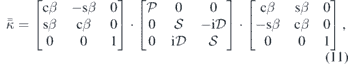
where cβ and sβ represent the cosine and sine of the angle β formed by the applied magnetic field B 0 with the z axis, and [59]


where:

are, respectively, the plasma frequency and (signed) cyclotron frequency of species s, and νs its damping frequency. At the frequency range of the device (a few GHz), the electron response dominates, and the other species (singly- and doubly-charged ions) can be safely neglected. The influence of νe on EM field propagation and absorption in the context of ECRTs was analyzed in [60]. There, it was shown that the actual value of the damping constant does not modify substantially the integrated power absorption at the resonance, and its only major effect was to thicken the absorption region. In the present model, νe is the effective electron collision frequency (i.e. the sum of the collision frequencies with the heavy species) from the E-module.
Combining equations (8) and (9) to eliminate  , one finds the inhomogeneous Maxwell's wave equation also referred to as the double-curl wave equation for the electric field:

where  is the wave number in vacuum.
The weak form of equation (16) is [61]:
where Ω, ∂Ω are the simulation domain and its enclosing boundary,  is a trial (i.e. weight) function, and ∗ denotes the complex conjugate transpose. In this work, we decompose the fields in azimuthal modes of mode number m, such that
  . As the ECRT exhibits axisymmetry, the only azimuthal mode of interest for this study is the purely axisymmetric mode m = 0. The field
  is expanded using a mixed basis of shape functions:

where N i are Nédélec (edge) functions and Pj are Lagrange (nodal) functions, i, j are indices that run for all edges and nodes, respectively, and ai , bj are the complex expansion coefficients for the meridian and azimuthal electric field. This decomposition is known to avoid spurious solutions present in other FE formulations of Maxwell equations [60–62].
The second term of equation (17) must be evaluated at the boundary of the domain. On the thruster walls the effect of the thin layer of boron nitride on the high-frequency fields is ignored, and the metal behind is treated as a perfect electric conductor,

resulting in homogeneous Dirichlet conditions on both Nj and Pj . Condition (19) is also applied to the core and shield of the simulated segment of coaxial cable. Natural boundary conditions are applied on the downstream and lateral boundaries of the plasma plume:

At the axis, axisymmetric boundary conditions [62, 63] are prescribed:

Lastly, to model the input of high-frequency EM power into the domain, a lumped port condition [64] is set upstream of the coaxial cable (at z = −2λ0), between the core and the shield conductors, which are electrically connected to the inner rod element and the lateral thruster wall, respectively. As a result, the transverse electromagnetic mode (TEM) is excited in the coaxial cable that delivers power to the plasma inside the thruster, and allows for any reflected power to return unimpeded through the coaxial.
Substituting equation (18) into (17), and using Galerkin's approach so that the same functional space is chosen for  than for
  , we construct a sparse square linear problem for the coefficients ai
and bj
. The modular finite element methods (MFEM) library [65] is used to construct the matrix and obtain the solution.
, we construct a sparse square linear problem for the coefficients ai
and bj
. The modular finite element methods (MFEM) library [65] is used to construct the matrix and obtain the solution.
The absorbed power density Qa can be computed as the real part of the scalar product between the high-frequency plasma current and the high-frequency electric field, which after some manipulation yields:
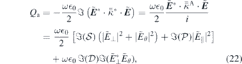
where  is the antihermitian part of
  associated to the presence of νe in equations (12)–(14) and is the only contribution of the dielectric tensor to include power absorption by the plasma.
The W-module uses an unstructured triangular mesh that allows reproducing complex geometries and also to locally refine the mesh as needed. A sketch of the W-module mesh is shown in figure 3(c). The open-source software Gmsh [66] is used for the mesh generation. As shown in sections below, the high-frequency field solution features substantial differences among regions of the domain due to the existence of qualitatively distinct propagation regimes, which depend on the electron density ne and applied magnetic field
B
0. The transition from one region to another is delimited by a cut-off and/or resonance surface. In each propagation regime, zero, one or two EM modes may exist, and the characteristic wavelength may vary substantially for each mode and with the propagation direction. In order to keep the number of mesh elements per wavelength Nλ
constant across the simulation domain, the mesh size is adapted for each region. A local minimum wavelength is estimated at each point of the domain from the dispersion relation of each principal propagating mode. The most restrictive regions in terms of minimum wavelength are seen to be the vicinity of the ECR and then the upper-hybrid resonance (UHR) region [59]. The mesh size is then computed according to this minimum wavelength, so that Nλ
> 20 across the simulation domain. This scheme is seen to stabilize and converge the fields close to these resonance surfaces, which at low mesh resolution can display numerical noise. A finer mesh size is also used near domain boundary corners and the coaxial to thruster chamber transition. The refinement and numerical verification of the W-module, discussed in appendices
2.4. Simulation setup
The ECR thruster used for this simulation is that of the MINOTOR prototype being matured at ONERA, as shown in figure 1. The applied magnetic field generated by an annular permanent magnet is shown in figure 3(b), whose local unit vector points downstream, defining magnetic streamlines. The operational point is the nominal one for the device [11, 16]. The geometric, operational, and numerical parameters are listed in table 1. The ECR surface is located approximately 3 mm downstream the backplate.
Table 1. Geometrical, operational and simulation parameters.
| Parameter | Name | Units | Value |
|---|---|---|---|
| lr | Inner rod length | cm | 2 |
| rr | Inner rod radius | cm | 0.115 |
| L | Lateral wall length | cm | 1.51 |
| R | Lateral wall radius | cm | 1.375 |
| Lp | Plume domain length | cm | 4 |
| Rp | Plume domain radius | cm | 2.75 |
| zinj | Injection surface center z | cm | 0.0 |
| rinj | Injection surface center r | cm | 0.5735 |
| tinj | Injection surface width | cm | 0.229 |
| rc | Coaxial shield radius | cm | 0.3 |
| f | Wave frequency | GHz | 2.45 |

| Neutral mass flow rate | mg s−1 | 0.2 |
| Pf | Input power | W | 30 |
| ΔtI | I-module timestep | ns | 10 |
| ΔtE | E-module timestep | ns | 0.25 |
| ΔtW | W-module update timestep | μs | 50 |
| uinj | Propellant injection velocity | m s−1 | 300 |
| Tinj | Propellant injection temperature | eV | 0.02 |
| αt | Anomalous transport coefficient | — | 0.02 |
| Nel,I | PIC mesh's cell number | — | 3360 |
| Nel,E | MFAM's cell number | — | 2550 |
| Nel,W | Wave mesh's cell number | — | 120 782 |
The instantaneous plasma properties computed in the coarser PIC mesh and the MFAM are smoothed using a Gaussian filter when interpolated to the EM mesh, and conversely, spatial anti-aliasing is applied when transporting Qa from the W-mesh to the MFAM.
The I-module has a timestep of ΔtI, which ensures that the fastest ion particles do not cross more than half a cell of the PIC mesh per timestep. The E-module is run 40 times per I-module step. Since the electron density ne and effective collisionality νe vary only slowly as the steady-state is approached, the W-module is only run every 5000 I-module steps.
To initialize the simulation, the I-module is run alone for a number of steps to fill the domain with particles, using a simplified, Boltzmann-relation model to emulate the electron response. Then, the E-module is activated with a uniform Qa map for an additional number of initialization steps. Finally, the coupled I-, E-, and W-modules are run together until steady state conditions are reached. Convergence of the plasma variables to steady state conditions is achieved already after 1.5 ms of simulation time. The simulation results of next section are shown at the end of the simulation, at 3.5 ms. Figure 4 illustrates the initialization and steady-state convergence of the simulation by plotting the computed thrust contributions of the different species. The updates of the power absorption profile are indicated by vertical dashed lines.
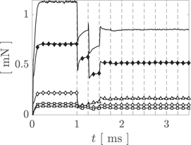
Figure 4. Evolution with simulation time of the thrust contributions (see equation (26) in section 3.4) of Xe+ (filled diamond), Xe2+ (diamond), Xe (square), e− (triangle) and the total (solid). After an initialization time of 1 ms, Qa is updated every 250 μs (dashed).
Download figure:
Standard image High-resolution imageIn the following sections, all plasma variables shown have been averaged over 500 ion module time steps after reaching the converged state to reduce numerical noise.
3. Results and discussion
The steady-state solution arising from the three coupled modules is reported and discussed next for the nominal operating point of the ECRT. Firstly, the resulting plasma properties are presented, including the singly-charged ion velocity and streamlines and the main contributions to electron momentum balance. Secondly, we explain the high-frequency fields and the power absorption density profile, and its connection with the solution of the transport properties. Thirdly, the plasma fluxes to the device walls are analyzed. Fourthly, the thruster integral figures of merit are computed and compared against the available experimental data for this thruster.
3.1. Quasi-steady plasma transport properties
In the steady-state, the neutral propellant density nn peaks at 6.5 × 10¹⁹ m−3 near the injection port (see figure 5(a)). Then, it decreases away from this location featuring a nearly homogeneous profile inside the thruster chamber, adding the contribution of ion recombination at the walls. Neutral density decreases as neutrals expand downstream and ionization takes place, falling more than two orders of magnitude downstream. This decrease is most evident close to the injector, where the ionization is dominant. Neutral density is lowest in the peripheral plume, essentially out of reach for the ballistic neutrals. The fraction of propellant mass flow rate leaving the discharge chamber as ions is roughly 50%.

Figure 5. Quasisteady plasma transport results: (a)–(d) are neutrals, singly-charged ions, electrons and doubly-charged ions densities, respectively, (e) and (f) electron temperature and pressure, (g) electrostatic potential and (h) singly-charged ions meridian velocity.
Download figure:
Standard image High-resolution imageThe singly- and doubly-charged ion densities, ni1 and ni2, are shown in figures 5(b) and (d). As it can be noted, ni1 is about one order of magnitude greater than ni2, and both follow the same overall behavior. The maximum singly- and doubly-charged ion densities are of the order of 9.5 × 10¹⁷ m−3 and 9.6 × 10¹⁶ m−3, respectively. The peak densities are reached in the vicinity of the injector, where most of the ionization takes place. Ion densities decrease toward the thruster walls, and ions impacting there are recombined into neutrals. The ion densities drop noticeably around the inner rod element and in the magnetic tube that originates in this region, which coincides with the region of higher electron temperature as discussed further below. This feature of the plasma discharge was observed to be robust to a sensitivity analysis of the simulation. Consistently with ni2 ≪ ni1, the electron density ne, shown in figure 5(c), is essentially equal to ni1, peaking around 1.1 × 10¹⁸ m−3. The electron density decreases downstream along magnetic lines as the plasma expands, reaching values of 2.7 × 10¹⁶ m−3 at the symmetry axis at the end of the simulated MN domain. This value is consistent with estimations performed with other models as the quasi 1D model presented in reference [55].
The quasi-steady map of electron temperature Te is shown in figure 5(e), with dashed lines indicating magnetic lines for reference. Due to the strong electron magnetization, effective energy transport rates of electrons along and across magnetic field lines are markedly different. While there exists large temperature gradients perpendicular to the applied magnetic field B 0, a near-isothermal behavior is observed in the parallel direction, at least in the finite domain simulated here. Gradual parallel cooling of electrons is expected further downstream, an aspect of the electron expansion that requires a kinetic treatment to be modelled consistently [67].
The maximum electron temperature is 43 eV and is found near the dielectric window that connects the thruster chamber with the coaxial cable, and in the magnetic tube that emanates from this location. As discussed later, the neighborhood of this window is also the location of the maximum power absorption. The electron temperature close to the symmetry axis is around 28 eV which is consistent with the experimental values reported by Lafleur et al [68] and later by Correyero et al [55] for 0.2 mg s−1 and, 20 and 30 W of absorbed power, respectively. Te goes below 4.3 eV at the lateral wall of the thruster and close to 0.2 eV at the top of the external wall.
Further insight on the electron dynamics can be gained by inspecting the electron pressure pe = ne Te, shown in figure 5(f). This variable is directly related to the thrust of the device, and with the quasi-steady electric field and azimuthal plasma currents, as discussed further below. While ne displays a minimum in the neighborhood of the axis of symmetry and Te presents a strong radial gradient, pe shows a relatively smooth behavior in the whole discharge. Looking at z = const sections of the thruster, the peak pressure takes place at a mid radius inside the annular chamber. Further downstream, in the MN, the maximum pressure is found closer to the axis of symmetry.
The quasi-steady plasma potential ϕ in figure 5(d) presents an axial fall of roughly 50 V within the simulation domain. It must be noted that the expansion will continue further downstream of this domain to infinity with collisionless electron cooling and further potential drop. The maximum value of ϕ is found inside the discharge chamber, close to the inner rod element of the thruster, right before the quasineutral pre-sheath decreases its magnitude toward the thin non-neutral wall sheaths. The potential decreases axially, along the MN. Note that the position of the maximum does not coincide with either the maximum of ne, Te, nor pe. In the direction perpendicular to the magnetic lines, and always in the quasineutral domain, the potential is essentially flat, except close to the inner rod element where it drops several tens of volts. A minor, secondary maximum of ϕ can be seen close to the lateral inner corner of the discharge chamber, which is attributed to this corner region of being essentially magnetically isolated from the rest of the plasma by the applied field lines, which means that electron transport into this region is severely limited; the small potential rise in this part of the device enhances electron transport from the rest of the plasma toward this region. Similarly, the small increase of ϕ at the top-left corner of the plume domain is attributed to the lack of electrons in this second magnetically-isolated region, although in this case it is considered a numerical side-effect of the finite simulation domain and the presence of the lateral plume boundary.
Another aspect of interest of the ϕ-map is that the potential fall along each magnetic line is not proportional to the corresponding value of Te, as could perhaps be expected. If this were true, a higher potential fall would be observed in the magnetic tube close to the inner rod element of the thruster. On the contrary, the potential fall is smooth and roughly the same across magnetic lines, indicating that the expansion is a global phenomenon for the whole plasma, despite electrons being well-magnetized. This behavior is consistent with the profiles of ne and Te of figures 5(c) and (e). Indeed, to leading order, the projection of equation (2) along 1∥ yields a Boltzmann-like relation for each magnetic line within the simulated domain,

where the subindex 0 represents values at a reference location for each line (e.g. upstream). As Δϕ = ϕ − ϕ0 is roughly identical for all magnetic lines, the relative drop of ne is smaller along the lines where Te is larger.
The singly-charged ion meridian velocity u i1 and their streamlines are shown in figure 5(h). While electrons are magnetized, the heavy ions are essentially unmagnetized and thus their dynamics is dominated mainly by the quasi-steady potential ϕ, which accelerates them downstream. Observe that ion streamlines (which roughly correspond to individual ion trajectories, since ions are relatively cold) do indeed not coincide with magnetic lines, and that the ion flow detaches inwardly from the magnetic field [69], resulting in less divergence than the expected one for fully-magnetized ions [70]. The resulting mean velocities at the last section of the simulation domain range from 3 km s−1 (at the axis) to 6 km s−1 (at the periphery). This difference is attributed to the location where the ions are created and the path they follow inside the ionization chamber before entering the MN region. For comparison, laser induced fluorescence (LIF) measurements of the ECRT operating at nominal conditions [55] indicate ion velocities of about 7 km s−1 and 11 km s−1 at 4 and 12 cm downstream the thruster exit, respectively. In addition, laser induced fluorescence (LIF) measurements obtained at Michigan [71] with a similar prototype report velocities around 9 km s−1 4 cm downstream the thruster exit plane, at background pressure of 13 μTorr.
As a derived quantity, the meridian Mach number of singly-charged ions, based on the approximate local sound velocity,  , features its maximal values (around Mi1 = 3) in the peripheral region of the plume, while at its core Mi1 is only slightly larger than 1. This radial variations are due to the differences in
u
i1, compounded with the variations in electron temperature Te. Arguably, the supersonic expansion in the MN of the device is uneven. It seems plausible that the presence of the rod element in the ECRT discharge chamber induces a dip in the ion Mach number in its wake. This behavior was seen to be robust against the sensitivity analysis carried out, and will be subject of future studies.
, features its maximal values (around Mi1 = 3) in the peripheral region of the plume, while at its core Mi1 is only slightly larger than 1. This radial variations are due to the differences in
u
i1, compounded with the variations in electron temperature Te. Arguably, the supersonic expansion in the MN of the device is uneven. It seems plausible that the presence of the rod element in the ECRT discharge chamber induces a dip in the ion Mach number in its wake. This behavior was seen to be robust against the sensitivity analysis carried out, and will be subject of future studies.
Lastly, it can be observed that inside the discharge chamber part of the ion streamlines precipitate onto the walls of the thruster guided by the electrostatic potential fall near those surfaces, giving rise to wall losses, which are discussed in section 3.3.
The quasi-steady state azimuthal electron and ion currents are an essential aspect of the operation of the device, as their interaction with the applied magnetic field B 0 is responsible for the generation of magnetic thrust and the cross-field confinement of the plasma. Figure 6 displays the azimuthal current of electrons jθe = −ene uθe, which is more than two orders of magnitude greater than the azimuthal current of any ion species.

Figure 6. Electron azimuthal current density. The black contour line shows the location of the sign change. Icons ⊕ and ⊖ represent the regions of positive and negative currents, respectively.
Download figure:
Standard image High-resolution imageTo leading order, in the perpendicular direction the electron pressure gradient −∇pe is compensated by the electrostatic force density ene∇ϕ and the magnetic force, jθe B0 1⊥ (see equation (2)),

Given that the quasi-steady electric potential is essentially flat across the magnetic field lines, the current jθe is responsible for most of the cross-field confinement of the electron pressure pe. Consequently, the sign of jθe switches mid-radius, close to where the maximum pe is found in the perpendicular direction, following the sign of −∇pe.
The reaction to the axial magnetic force density, jθe Br0, is felt on the coils of the thruster, and is termed magnetic thrust. Since in the present simulation Bz0, Br0 > 0 in the domain, only negative jθe results in positive thrust generation. It can be seen that the outermost part of the plasma is the main contributor to magnetic thrust, while the electrons close to the inner rod element of the device cause some negative magnetic drag in order to confine the electron pressure away from this element. This is a consequence of the maximum electron pressure being located at an intermediate radius rather than the axis of symmetry, and is likely an effect of the presence of the inner rod element. Downstream of this rod element, a small localized region with jθe < 0 is found.
3.2. Fast electromagnetic fields and power absorption
The solution to the high-frequency EM fields depends on the excitation frequency ω, the applied magnetic field B 0, the electron density ne, and the collisionality νe. In particular, the first three variables determine the field propagation regimes, the cut-offs, and the resonances. The last variable, νe, which ranges from a maximum value of 4.5 × 10⁸ Hz inside the source and decreases downstream, affects mainly to the homogeneity of the power absorption map. Notably, while B 0 is an input to the simulation, ne and νe depend dynamically on the plasma transport solution.
The different EM parametric regions in steady-state are shown in figure 7(a), following the numerical nomenclature (I to VIII) of Stix [59]. The right-hand circularly polarized wave (R) resonates when ω = eB0/me which determines the critical value of B0 (875 G) and the location of the ECR surface. This value separates regions I through V from regions VI through VIII. The plasma frequency cut-off occurs when ω = ωpe, which determines the critical value of ne (=7 × 10¹⁶ m−3). Regimes I, II, III, and VI take place below this value of ne, and are considered underdense regimes. Regimes IV, V, VII and VIII are overdense regimes. Region I (low B0, low ne) is topologically equivalent to propagation in vacuum, with both R and L (i.e. left-hand circularly polarized) propagating modes. It is separated from region II by the R wave cut-off. In region II, only L waves propagate. As B0 and ne increase, eventually the UHR is crossed into region III, where two propagating solutions exist at directions other than B 0. Region IV (low B0, high ne) exhibits propagating L waves only. In region V (separated from region IV by the L wave cut-off) no propagating solutions exist, and all EM fields are evanescent. Region VI (high B0, low ne) features both R and L polarizations. Regions VII and VIII (high B0, high ne) feature whistler R waves, which propagate in directions close to B 0; additionally, region VII also has regular L-waves.

Figure 7. (a) EM field propagation parametric regions with contours representing the boundary surfaces and (b) minimum principal wavelength, computed from the local dielectric tensor.
Download figure:
Standard image High-resolution imageAs it can be noticed in figure 7(a), in this ECRT simulation all these regions (i.e. I through VIII) are present within the simulation domain and in close proximity to each other. The contour lines detail the location of the different cutoffs and resonances, which act as the boundary surfaces of the different propagation regimes. In particular, the presence of the ECR and UHR stands out. Whereas the location of the ECR is fixed only by the magnetic field, the UHR is determined by a combination of both the magnetic field and the electron density.
As the EM power enters the discharge chamber through the coaxial line, it enters regions VI–VIII (upstream of the critical B0), and soon reaches the ECR surface. Most of the discharge chamber is overdense (ωpe > ω), and therefore downstream of this surface there is a region V where only evanescent fields are allowed. However, a thin low-density channel exists near the inner wall corresponding to regions III and IV. Power can propagate along this channel, and also tunnel through a short evanescent region. Further downstream, as both B0 and ne decrease, all other regions are crossed, until eventually region I is reached.
The existence of all these regions implies wide changes of the local wavelengths in the domain. Figure 7(b) illustrates this by plotting the minimum wavelength in the perpendicular and parallel directions for all propagating modes. The smallest wavelengths occur near the ECR and the UHR surfaces, and the W-module mesh has been refined accordingly, as described in section 2.3 and appendix
The amplitudes and complex phases of the three components of the fast electric field
E
are shown in figure 8. The resulting electric field inside the coaxial cable is a strong radial field, characteristic of the TEM mode. As the power flows into the plasma, the radial component of the EM wave electric field  still dominates on both sides of the ECR surface, and continues to be large in the thin regions III and IV that exist around the rod element of the thruster. It can be observed that an axial electric field
  also develops before the ECR surface and downstream from the rod element decaying after the resonance, and that the azimuthal field
  plays only a minor role. Small magnitude fields also exist downstream, around the UHR surface.
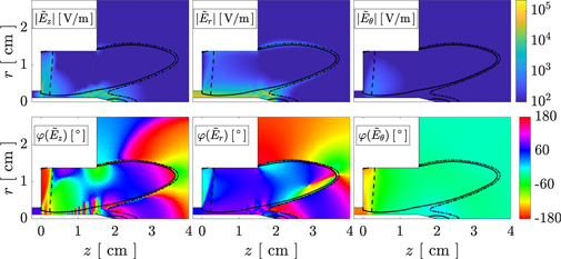
Figure 8. EM wave electric field (complex magnitude and phase). The contour lines represent the cutoff ω = ωpe, the ECR surface (dashed) and the UHR surface (dashed–dotted).
Download figure:
Standard image High-resolution imageThe phase plots in figure 8 indicate that no major wave structures exist in the domain, which would be evidenced by alternating phase structures, given its small size compared to the electric length in vacuum; the only exception is in the narrow propagation channel close to the inner rod element, where a short-wavelength mode is observed in  . No major standing-wave structures are observed within the simulation domain, indicating that reflection at the free surfaces downstream is small.
The power absorption density Qa is shown in figure 9. Absorption occurs mainly at around the ECR surface, as expected. The power absorption has its maximum at the ECR, near the inner rod element of the thruster. Some power absorption also takes place around the inner rod, in the propagating channel. Overall, most of the power is deposited in the magnetic tubes close to the inner rod, which is also where electron temperature features its peak values. The absorption at the downstream UHR surface is non-zero, but orders of magnitude smaller.

Figure 9. EM power density absorbed by the electron species.
Download figure:
Standard image High-resolution imageThe absorption map can be explained by inspecting the magnitude of the different terms in equation (22). As the applied magnetic field is mostly axial in the device,  and
and  . At the ECR surface, the imaginary part of
  features its maximum and it is two orders of magnitude greater than the imaginary part of
  . As
. As  , the power absorption density Qa is therefore dominated by the term

This term reaches its peak value close to the exit of the coaxial line, where the radial electric field is larger and the ECR surface is found, and consequently this is where the higher Qa occurs. Lastly, it is noted that while absorption at the resonance requires νe > 0, the actual value of this parameter only influences the thickness of the resonance layer, while the integrated power deposited in it is essentially unaffected [60].
3.3. Particle and energy wall fluxes
Figure 10(a) displays the particle flux to the thruster walls for each species, as a function of arc-length variable ζ, introduced in figure 1. This variable starts at the tip of the inner rod, goes around clockwise along the thruster wall meridian section, finishing at the end of the external wall.

Figure 10. (a) Particle flux, (b) net energy flux and (c) average impact energy of the different species to the thruster walls: electrons (triangles), Xe+ (filled diamonds), Xe2+ (diamonds), and Xe (squares).
Download figure:
Standard image High-resolution imageThe internal thruster walls sustain a much larger particle flux than the external walls, differing in several orders of magnitude. Singly- and doubly-charged ion particle fluxes evolve similarly with ζ, being the former always greater than the latter. Singly-charge ion particle flux features values between 1019 and 1021 m−2 s−1 flux, peaking around the middle of the rear wall, where the injector is located and ions density is maximum. Neutral flux to the walls is shown in the figure for comparison. Amongst all the regions inside the thruster chamber, the corner region between the rear and lateral wall collects the least amount of ions. All corners exhibit a discontinuity motivated by the change in normal vector but this corner region features enhanced magnetic shielding. As a result insufficient electron temperature in the vicinity of this region, ionization is poor there, and combined by the strong magnetization results in a repelling electrostatic field that limits the ion flux to the walls significantly. The primary electron flux follows a similar behavior to the singly-charged ions both at the lateral wall and backplate. Nevertheless, approaching the inner rod wall, the flux increases by more than an order of magnitude reaching values of about 1022 m−2 s−1.
At each location along the (dielectric) walls, the net flux of negative and positive charges to the wall must be equal. The large difference between the fluxes of electrons and ions toward the inner rod wall is indicative of the large SEE that takes place there, where indeed the yield δws, motivated by the considerable electron temperature, is close to unity. The difference of the fluxes decreases to near zero along the back, lateral, and external walls, where electrons are cooler and SEE becomes less important.
Figure 10(b) shows the total net energy flux to the walls of each species. This magnitude is relevant to understand the thermal loads endured by the exposed walls. The maximum energy load is exhibited at the inner rod. Electrons dominate the energy flux to this element, due to the high SEE, and are comparable to the ion energy flux in other walls. Singly-charged ions have a larger energy flux with respect to doubly-charged ions everywhere due to their significantly higher density. The maximum ion energy flux is 0.8 W/cm2, and occurs at the injector location, near the region where most ionization takes place. As could be expected, the corner region of the thruster is clearly well shielded magnetically, not only from a particle flux viewpoint as reported above, but also from an energy viewpoint.
Finally, figure 10(c) portraits the average impact energy per particle of each species. This variable is relevant in erosion studies, as the impact energy must be greater than a material dependent threshold energy for sputtering to take place. In this case, we see that doubly-charged ions are responsible for the highest per-particle energy deposition to the walls. This is due mainly to their double-charge acceleration in the wall sheaths; indeed, the sheath accounts for most of the impact energy for both singly- and doubly-charged ions everywhere. Energies ranging from roughly 10–20 eV to 200–300 eV are computed. The maximum impact energy takes place at the end part of the rod element, where experiments report the largest and fastest erosion under operation. Specific electron energy is small except on the inner rod element. Neutrals impact energy is negligible.
3.4. Propulsive performance
The thrust F of a MN-based thruster is generated partially inside the source, but mainly in the MN region, which extends to infinity. In the present simulation, F is computed by integration of the plasma momentum on the free boundaries of the domain ∂Ωf,

where the sum on s extends to all species. The thrust F can be divided in two contributions:

and

which equal the sum of all the axial dynamic pressure force of each species s on the thruster walls ∂Ωw and the axial magnetic force produced by the azimuthal plasma current on the thruster magnets, respectively [21]. It should be noted that the expansion continues further downstream, beyond the computational domain, and therefore a small part of the generated thrust is missed by the simulation. Indeed, the major part of ion acceleration in this thruster occurs in the first few cm after the thruster chamber exit [55], and therefore is captured here. The specific impulse is calculated from this magnitude as  .
.
The microwave power entering the thruster, Pf, is partially absorbed by the plasma, Pa, and partially reflected back through the coaxial cable, Pr, thus

Notice that in the present simulations there are no free-space radiation losses; this is representative of the operation of the device inside a laboratory vacuum chamber, where the radiated power is confined.
The reflected power is obtained directly from the voltage standing wave ratio (VSWR), computed as the ratio of the maximum and minimum values of the radial electric field in the coaxial cable, and is directly related to the power coupling efficiency ηp as

Observe that the reflected power cannot be considered a priori a loss mechanism, as this power can be recirculated back to the thruster quite efficiently by impedance matching in the microwave circuit design. Nevertheless, a large reflection ratio would be symptomatic of an inadequate power coupling to the plasma.
Following [47], the power balance for all plasma species can be expressed as

where Pexc and Pion are the power spent in excitation and ionization of the propellant; Pwall is the kinetic, thermal, and heat flux power lost to the walls; and Pp is the power flux of all species through the free boundaries. Consequently, we can define the loss ratios  exc = Pexc/Pa, ion = Pion/Pa, and wall = Pwall/Pa.
The (overall) thruster efficiency is computed as

This efficiency can be approximately decomposed as

where  is the utilization efficiency, i.e. the fraction of propellant mass flow rate that reaches the domain free boundaries as ions (
 ); ηe = Pp/Pa refers to the energy efficiency, i.e. the fraction of absorbed power that becomes plume kinetic and thermal power (Pp); ηc = Pi/Pp is the conversion efficiency, i.e. the portion of the plume power in the form of kinetic ion power (Pi); finally, ηd = Pzi/Pi is the divergence efficiency, i.e. the fraction of ion kinetic power which in the axial direction (Pzi), thus generating thrust. The difference in equation (33) between ηF and the product ηu
ηe
ηc
ηd is due to the difference between Fi and F, which in a completely developed expansion is expected to be small. However, in the present simulation with finite domain, the electron contribution to thrust accounts for up to a 25% (see figure 4) at the free downstream boundary. This suggests that the expansion is incomplete by z = 4 cm, and that additional thrust is to be gained further downstream as the MN continues to convert electron power into directed ion kinetic power.
); ηe = Pp/Pa refers to the energy efficiency, i.e. the fraction of absorbed power that becomes plume kinetic and thermal power (Pp); ηc = Pi/Pp is the conversion efficiency, i.e. the portion of the plume power in the form of kinetic ion power (Pi); finally, ηd = Pzi/Pi is the divergence efficiency, i.e. the fraction of ion kinetic power which in the axial direction (Pzi), thus generating thrust. The difference in equation (33) between ηF and the product ηu
ηe
ηc
ηd is due to the difference between Fi and F, which in a completely developed expansion is expected to be small. However, in the present simulation with finite domain, the electron contribution to thrust accounts for up to a 25% (see figure 4) at the free downstream boundary. This suggests that the expansion is incomplete by z = 4 cm, and that additional thrust is to be gained further downstream as the MN continues to convert electron power into directed ion kinetic power.
In addition to these partial efficiencies, another relevant quantity is the production efficiency, defined as the ratio of ion flow rate at the free boundaries with respect to that at all the simulation boundaries including thruster walls,

which is closely related to the number of times each atom undergoes reionization, and characterizes the plasma losses to the walls.
Table 2 displays the performance figures of the simulation. For comparison purposes, the available experimental data from ONERA thruster are also shown. The total thrust produced by the thruster in the simulation is 0.84 mN, and the specific impulse 428 s, which show a great agreement with the experimental measurements. The fraction of magnetic thrust to total thrust amounts to approximately 62%, which again agrees well with the available experimental data [72]: 60% for the device operating at 0.2 mg s−1 and 40 W.
Table 2. Thruster performances. Values at the thruster (*) are computed from the data reported at reference [11] (before the vacuum chamber feedthrough) with the estimated 2 dB losses between that point and the thruster, as indicated in that reference.
| Parameter | Name | Units | UC3M | ONERA [11] |
|---|---|---|---|---|

| Mass flow rate | mg s−1 | 0.2 | 0.2 |
| Pf | Input power | W | 30 | 53.7* |
| F | Thrust | mN | 0.840 | 0.850 |
| Fp | Pressure thrust | mN | 0.322 | — |
| Fm | Magnetic thrust | mN | 0.518 | — |
| Pa | Absorbed power | W | 26.9 | 27.9* |
| Pr | Reflected power | W | 3.1 | 4.28* |
| Isp | Specific impulse | s | 428 | 429 |
| Ii | Ion current | A | 0.082 | 0.065 |
| ηF | Thrust efficiency | % | 6.6 | 6.5* |
| ηprod | Production efficiency | % | 40.9 | — |
| ηu | Utilization efficiency | % | 50 | 45.1 |
| ηe | Energy efficiency | % | 25.3 | — |
| ηc | Conversion efficiency | % | 32.2 | — |
| ηd | Divergence efficiency | % | 91.2 | — |
|
exc
| Excitation losses | % | 4.8 | — |
|
ion
| Ionization losses | % | 7.0 | — |
|
wall
| Material wall losses | % | 63.0 | — |
| VSWR | Voltage ratio | — | 1.8 | 2.15* |
| ηp | Power coupling eff. | % | 91.8 | 86.7* |
In reference [11], efficiencies are computed with respect to the transmitted power (i.e. ηp Pf) and that this power includes the power losses in the cables, the feed-through, the DC block and the connectors/adapters, which are of the order of 2 dB. Table 2 shows the efficiencies and powers, taking into account the reported attenuation losses between the measurement location (prior to the tank) and the thruster. The thrust efficiency is very similar in the simulations and the experiments, around 6.6%.
The main inefficiency arises from plasma losses to the walls. First, the fraction of generated ions that become plume ions, given by ηprod, is quite low, about 41%, while the rest of them are recombined at the walls. Second, the energy efficiency is rather low, ηe ≈ 25%. While excitation and ionization losses (measured by exc and ion) are arguably small, about two-thirds of the absorbed power (wall) is lost to the walls, transported by the ions and electrons that impact on them. In fact, the integrated energy fluxes (see section 3.3) over the inner thruster walls areas adds up to 16.9 W, where 51% is lost through the inner rod surface, 40% through the backplate, 9% through the lateral wall and 0.1% through the external wall. Large losses at the magnetically unshielded backwall are well-known from HPT analyses [21, 73] and the way to reduce them would be to shield that wall (without altering much the wave propagation). Magnetic shielding seems to operate rather well at the lateral wall; it does not behave well at the rod due to the large electron temperatures around it, leading to very large thermal loads in that thin element, which amounts for only a 6% of the total inner thruster walls area. To reduce this problem should be a central task of any design optimization of the thruster chamber.
The second main source of inefficiency is related to the meager utilization efficiency, a 50% in the simulation, and also in good agreement with the experimentally-obtained value. These values are also common in HPTs [74] and are likely due to the large wall recombination. The consequence is that a large fraction of the propellant is leaving the source as neutrals, generating essentially no thrust.
On a positive note, the divergence efficiency ηd of 91.2% shows that the kinetic power of ions leaving the domain is mainly axial and that good magnetic detachment takes place in the MN. On the other hand, and in line with the discussion above, the rather low conversion efficiency ηc evidences that the expansion is still incomplete in the simulation domain.
The experimentally-reported power coupling efficiency ηp is close to unity already in early designs [4] and in contemporary ones [18], where they report a 95%. These values are measured between the microwave generator and the microwave feedthrough on the tank, and therefore do not record the attenuation in the line from the tank feedthrough to the thruster. With the estimated power attenuation factor of 2 dB given in [11], the actual coupling efficiency at the thruster entrance for the prototype simulated here is 87%. This value is close to the computed 92% coupling efficiency.
4. Conclusions
An axisymmetric model of the plasma discharge in an ECRT has been presented, which couples together the slow plasma transport and the fast EM fields. Self-consistent simulation results for a thruster of this type have been reported, discussed, and compared with existing experimental data from the MINOTOR ECRT prototype operating at its nominal point.
Results reveal the mutual dependency between the quasi-steady plasma properties and the high-frequency EM fields, as plasma density determines the propagation regimes and the location of cut-offs/resonances, while the power absorption map drives the electron temperature profile. Multiple EM propagation regimes coexist in the device. In most of the domain wave structures are not observed, which is expected due to the small dimensions of the thruster. The exception is the neighborhood of the inner rod element of the device, where a short wavelength mode has been found. The main contribution to EM power absorption is related to the radial electric fields at the ECR region, in particular those closest to the exit of the coaxial line. The ratio of reflected power is small. The field propagation beyond the ECR surface occurs along a low-density channel close to the inner rod element of the thruster. As the topology of these regions responds to the plasma density profile, varying the input mass flow rate or the input power is expected to alter them and consequently modify the EM power flow. The study of these variations will be subject of future work.
Large values of the electron temperature are observed in the magnetic tube that connects with the coaxial line exit. Electron temperature is almost uniform in the parallel direction to the magnetic field, but a large perpendicular gradient exists. The electron pressure profile, on the other hand, is smooth, not showing any pronounced peak. The plasma density profiles peak at an intermediate radius instead of at the axis of symmetry. This is likely a consequence of the presence of the inner rod, which makes the plasma density drop close to its surface.
The quasi-steady electric field developed by the plasma is quite similar along all magnetic lines in spite of the differences in electron temperature among them. This, combined with the observed ion velocity profile, results in a local ion Mach number that varies substantially among magnetic lines.
The particle and energy fluxes to the walls have been analyzed per species, showing that the inner rod of the thruster undergoes the largest particle and energy influx. This element has also shown to undergo the major part of the heat lost through the thruster walls. Thus, an alternative design choice for the geometry and the material of the inner rod element could lead to significant improvement of the overall thruster performances. Regarding the impact energy, the maximum is exhibited by doubly charged ions and overall it occurs at the inner rod element. Thus, this element not only will suffer from considerable thermal stress loads but also from the erosion provided by the energetic impact of ions.
The central part of the rear wall is essentially perpendicular to the magnetic field lines that expand into the MN region, and thus is connected to the bulk of the plasma discharge. Particle and energy fluxes to this part of the rear wall are large. On the contrary, the corner region between the rear and the lateral walls forms a nearly-isolated region which is well protected by the magnetic field, and this is reflected in the lower particle and energy flux to it.
The performance figures computed from the simulation results show a great agreement with existing experimental data, serving as a partial validation point for this numerical model. The main loss mechanisms are plasma losses to the walls, especially to the inner rod element, and a low propellant utilization. Given this agreement, and the difficulty of experimentally measuring detailed profiles as the ones obtained by the simulation, the present model could be used to propose novel designs that could optimize the overall thruster performance. Further work must continue to improve and validate the model, in particular running simulations in larger domains and using the available laboratory measurements of plasma properties.
Lastly, the numerical treatment of the fast EM fields near the ECR and UHR surfaces presents several difficulties, which have been addressed with a predictive local refinement strategy applied to the mesh of the W-module. Future work will look into other schemes to reduce the need of refinement in these regions.
Acknowledgments
The authors thank R Otín for the valuable and insightful discussions. Furthermore the authors thank S Shiraiwa, LE García-Castillo and A Amor for their useful suggestions in the development of the FE W-module, and A Domínguez-Vázquez who assisted the authors during the development of the simulations in the details related to the PIC module. The research leading to these results has been funded by the European Union H2020 program under grant agreement 730028 (Project MINOTOR). Part of A Sánchez-Villar funding came from Spain's Ministry of Science, Innovation and Universities FPU scholarship program with Grant FPU17/06352.
Data availability statement
The data that support the findings of this study are available upon reasonable request from the authors.
Appendix A.: W-module mesh refinement strategy
The different EM modes that exist in each region of figure 7 have widely varying characteristic wavelengths. Accurate simulation of the high-frequency EM fields demands a sufficient number of elements per wavelength, which calls for a specific W-module meshing strategy, driven by different requirements than the I-module and E-module meshes.
To illustrate the difficulty, figure 11 shows the complex phase of the fast EM fields  in a uniform mesh and a refined mesh. It also displays the characteristic number of mesh elements per local wavelength, this one computed from the dielectric tensor for each case. High wavenumber oscillations are observed in the neighborhood of the UHR surface in the uniform-mesh simulation results, which are only partially physical. Such oscillations do not correlate with waves as there is a mismatch between the expected wavelengths given by the local properties and the numerical solution. Furthermore, as the oscillations scale is of the order of the mesh-cell characteristic length, this suggests that such oscillations are in fact spurious noise. Indeed, progressive refinement of the mesh shows that the fields converge to those on the right of the figure, where most of these oscillations have disappeared and therefore are considered error noise. Only some of the oscillations remain in the low-density channel that occurs near the inner rod element in this simulation, as shown in the main text (figure 8). Noteworthily, while the noise affects the field phase, it was observed that it does not impact significantly the power absorption profile.
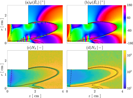
Figure 11. Complex phase of the Ez fast EM field and number of mesh elements per local wavelength for a uniform mesh (left) and for a refined mesh (right).
Download figure:
Standard image High-resolution imageTherefore, in the present work the mesh is refined around the ECR and the UHR regions in the last iterations of the W-module only, a procedure that has proved successful in mitigating this spurious noise and speeding up convergence to the steady-state results.
As a final observation, it is noted that multiple plasma and magnetic field profiles were tested, reaching the conclusion that the location of this noise is in direct correlation with the location of the UHR surface. Similar spurious solutions near this resonance are reported near lower-hybrid resonances in other works [75], which show some mathematical analogy with the UHR. A regularization of the double-curl formulation of the FEs scheme is suggested there as an alternative route to solve this issue [76, 77].
Appendix B.: W-module numerical verification
The W-module used for this simulations has been implemented based on a verified FE discretization library [65]. As for the EM problem to be solved, several unit and integration tests were performed to verify the EM solutions. In a first stage, the method of manufactured solutions [78] was used with simplified simulation setups [45]. The expected order of convergence was observed. Secondly, for a simulation domain and plasma properties similar to the ones shown in the main text, an error convergence analysis with different meshes was performed. The strategy used was to start with a coarse mesh and progressively refine the mesh by splitting each element into four, computing the solutions of the EM fields for each mesh. A total of five meshes are used, consisting of 465 and 119 040 elements the coarsest and finest meshes, respectively. Taking the finest mesh as the reference solution, the errors on the axial electric field norm and phase angle are shown in figure 12. Note that the amplitude error has been normalized by the maximum value in the domain. The obtained results serve to verify the convergence of the scheme and to quantify the error committed by the W-module as a function of the mesh size.

Figure 12. Absolute errors, mean (bluebars) and standard deviation (errorbars) in axial electric field amplitude and phase, for different numbers of consecutive mesh refinements.
Download figure:
Standard image High-resolution image