


Abstract
Nonlinear ion-acoustic waves, ion holes, and electron holes have been observed on the Parker Solar Probe at a heliocentric distance of 35 solar radii. These time domain structures contain millisecond duration electric field spikes of several mV m−1. They are observed inside or at boundaries of switchbacks in the background magnetic field. Their presence in switchbacks indicates that both electron- and ion-streaming electrostatic instabilities occur there to thermalize electron and ion beams.
Export citation and abstract BibTeX RIS

Original content from this work may be used under the terms of the Creative Commons Attribution 4.0 licence. Any further distribution of this work must maintain attribution to the author(s) and the title of the work, journal citation and DOI.
1. Introduction
Time domain structures (TDSs; electrostatic or electromagnetic electron holes, ion holes, solitary waves, double layers, nonlinear whistlers, etc.) are ∼1 ms pulses having significant electric fields parallel to the background magnetic field (Mozer et al. 2015). They are abundant through space, occurring along auroral zone magnetic field lines (Temerin et al. 1982; Mozer et al. 1997; Ergun et al. 1998), in the magnetospheric tail and plasma sheet (Cattell et al. 2005; Tong et al. 2018; Lotekar et al. 2020), at reconnection sites (Cattell et al. 2005; Steinvall et al. 2019; Lotekar et al. 2020), in the solar wind (Mangeney et al. 1999; Malaspina et al. 2013), in collisionless shocks (Wilson et al. 2010; Vasko et al. 2020; Wang et al. 2020), and in the magnetospheres of other planets (Pickett et al. 2015). TDSs are also expected along the Parker Solar Probe orbit (Mozer et al. 2020a). According to theoretical estimates and simulations (Cranmer & van Ballegooijen 2003; Valentini et al. 2011, 2014), these nonlinear structures can provide thermalization of electron and ion beams produced in the course of the turbulence cascade development at scales the order of the electron inertial length and down to the Debye length. This paper discusses such observations at a heliocentric distance of 35 solar radii. The electric field experiment on the Parker Solar Probe measures electric fields from DC to 20 MHz. A general description of the instrument and its electronics appears elsewhere (Bale et al. 2016). In this paper, the data from DC to 2 MHz are discussed. These measurements are obtained from the potentials of the four antennas, V1 through V4, that are located in the plane perpendicular to the Sun–satellite line. They produce E12 = (V1−V2)/3.5 and E34 = (V3−V4)/3.5, which are then rotated into the spacecraft coordinate system to produce EX and EY . The direction, X, is perpendicular to the Sun–spacecraft line, in the ecliptic plane, and pointing in the direction of solar rotation (against the ram direction), Y is perpendicular to the ecliptic plane, pointing southward, and Z points toward the Sun. The numerical factor, 3.5, is the effective antenna length (Mozer et al. 2020a). The uncertainties of the amplitudes of the waves and time domain structures reported in this paper are estimated to be about a factor of 2. These amplitudes are underestimated because the capacitive divider that couples the antennas to the electronics decreases the measured electric field relative to that on the antennas. They are often overestimated because short antennas produce overestimates of the electric field by factors of 2–4, as was observed during antenna deployment on the Cluster satellite and as is observed on the Parker Solar Probe from the ratio of the electric field to the magnetic field in whistlers.
2. Nonlinear Ion Acoustic Waves
Figures 1(b) and (c) present a 5 ms interval of the X and Y electric field components of a nonlinear wave. Evidence of nonlinearity is indicated by the nonsinusoidal waveforms of EX and EY in panels (b) and (c) and by the presence of the second harmonic in the spectra of panel (a) at a frequency of about 12,000 Hz. The fundamental wave frequency is above the electron gyrofrequency of 2100 Hz, as shown in panel (a) where the fundamental power in the nonlinear wave was about 6000 Hz. It was also below the Langmuir frequency of 100 kHz, as shown in Table 1.
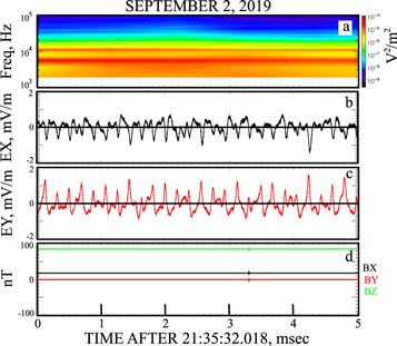
Figure 1. Nonlinear ion-acoustic waves observed on the Parker Solar Probe at 35 solar radii: (a) the spectrum of the electric field EX measured at 2 MHz; (b), (c) waveforms of electric field components EX and EY measured at 2 MHz; (d) background magnetic field. XYZ is the coordinate system with the z-axis pointing toward the Sun, while the x- and y-axes are in the plane of the electric field measurements. The data are presented in the spacecraft frame.
Download figure:
Standard image High-resolution imageTable 1. Plasma Parameters during the Events Described in This Paper
| Date | Density | Magnetic Field | Plasma Frequency | Electron Gyrofreq | Solar Wind Speed |
|---|---|---|---|---|---|
| (cm−3) | (nT) | (Hz) | (Hz) | (km s−1) | |
| 9/2/2019 0358 | 110 | 100 | 100,000 | 2100 | 400 |
| 9/2/2019 0825 | 80 | 90 | 70,000 | 2600 | 500 |
| 9/2/2019 2019 | 80 | 100 | 75,000 | 2300 | 440 |
| 9/2/2019 2135 | 180 | 100 | 120,000 | 2100 | 400 |
| 6/6/2020 0008 | 150 | 160 | 110,000 | 3000 | 470 |
Download table as: ASCIITypeset image
To discuss the mode of this nonlinear wave, Figure 2 presents the 2000–8000 Hz bandpass-filtered data of Figure 1 in order to study the fundamental frequency of the wave. Because the X and Y components of the wave electric field in panel (b) are about 180° out of phase, the wave is linearly polarized. This result, plus the absence of a measured wave magnetic field, requires that the wave be electrostatic. For this case, the electric field should be mostly parallel to the magnetic field and the magnetic field is mostly along the z-axis. Thus, Parker Solar Probe measures a relatively small projection of the wave electric field onto the X−Y plane. The unmeasured EZ component of the electric field was about 10 mV m−1, because EZ/EX ∼ BZ /BX ∼ 5 and EX ∼ 2 mV m−1.
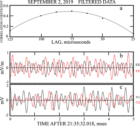
Figure 2. Bandpass-filtered nonlinear ion-acoustic waves of Figure 1. Panel (a) shows that the ∼75 ms time lag between observation of V1 and V2 corresponded to a wave speed similar to the ion thermal speed.
Download figure:
Standard image High-resolution imageTo distinguish whether the wave was an electron acoustic wave or an ion-acoustic wave, it is necessary to estimate the wave speed. This may be done by considering the time taken by the wave to go from V2 to V1 as the wave passes over the spacecraft. In panel (c), V2 leads V1 by an amount that is illustrated in panel (a), which is the cross-correlation of the two signals as a function of the lag time between them. This 75 ms lag is the time required for the wave to move from the tip of antenna-2 to the first surface at the spacecraft potential. Because of the complex geometry of the antennas and the spacecraft, this distance can only be estimated as 1–2 m. Assuming a distance ∼1 m, the speed deduced from these results is about 10 km s−1. This is, at most, the speed of the wave in the X−Y plane in the spacecraft frame. A better estimate of the total speed in the plasma rest frame is (10−vp · B /B), where vp is the plasma velocity in the spacecraft frame and we have taken into account that the wave propagates almost parallel to the local magnetic field, B . Because vp was ∼400 km s−1, this speed is a few hundred km s−1, which is the order of the ion thermal speed and is a factor of about 40 smaller than the electron thermal speed. Thus, this is a nonlinear ion-acoustic wave.
Linear, Doppler-shifted, ion-acoustic waves occur at the Parker Solar Probe frequently (Mozer et al. 2020b). Nonlinear ion-acoustic waves have been observed in the Earth's auroral zone (Temerin et al. 1979), but it is believed that these are the first such observations elsewhere in space. There are several theoretical discussions of nonlinear ion-acoustic waves in the literature (Shukla & Yu 1978; Lee & Kan 1981; Malfliet & Wieers 1996).
3. Ion Holes
Figure 3 presents a different effect associated with the linear ion-acoustic wave observed at the beginning of panel (b). This is an ion-acoustic wave because it is electrostatic and linearly polarized along the background magnetic field of panel (d) (since the ratio EX /EY is about equal to the ratio BX /BY ). Its speed was ∼100 km s−1, and it occurred at a frequency (panel (a)) that is an order of magnitude greater than the electron gyrofrequency of 2600 Hz and less than the plasma frequency of 70 kHz (see Table 1). This wave broke up into several time domain structures during the following 4 ms, and these structures moved parallel (or antiparallel) to the background magnetic field since the ratio EX /EY is also about equal to the ratio BX /BY .

Figure 3. A linear ion-acoustic wave that broke up into ion holes. The format of this figure is the same as that of Figure 1.
Download figure:
Standard image High-resolution imageFigure 4 illustrates the time domain structures of Figure 3 after being bandpass filtered between 1000 and 20,000 Hz. As is visible in panel (c), V2 leads V1 by about 30 μs, which is in accordance with the cross-correlation of panel (a). Thus, the speed of the time domain structure was about 30 km s−1 in the X−Y plane, in the spacecraft frame. Again, a better estimate of the total speed in the plasma rest frame is (30−vp · B /B) km s−1, where vp is the solar wind speed. This speed is a few hundred km s−1, which is the order of the ion thermal speed (for a 50 eV temperature) and is a factor of about 40 smaller than the electron thermal speed. Thus, these appear to be ion holes.
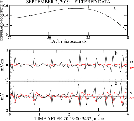
Figure 4. Low pass-filtered ion holes of Figure 3. Panel (a) shows that the time lag between V1 and V2 was about 30 μs, corresponding to a hole speed similar to the ion thermal velocity.
Download figure:
Standard image High-resolution imageThese results are summarized in Figure 5, which describes the situation along the x-axis. The magnetic field was along +X (Figure 3(d)) and, because V2 led V1, the structures moved in the +X direction (see Figure 1 of Mozer et al. 2020a for the antenna geometry). EX was first negative and then positive in Figure 4(b), as illustrated in Figure 5. As a result, the potentials of these structures were negative and they were moving at ∼ion thermal speeds in the plasma frame, so they were ion holes. It is also noted that they were moving sunward. The typical peak-to-peak temporal width of the ion holes was about 1 ms and the electric field amplitude was a few mV m−1. Because the velocity of the ion holes was 30 km m−1 in the spacecraft rest frame, the spatial scale of the ion holes was a few meters and the electrostatic potential of these ion holes does not exceed 0.01 V.
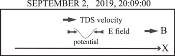
Figure 5. Geometry of the magnetic field, the ion hole velocity, and its electric field, showing that the ion hole had a negative potential and moved sunward.
Download figure:
Standard image High-resolution image4. Electron Holes
Figure 6 gives an example of time domain structures observed when BZ ∼ 0, such that the full electric and background magnetic field were measured in the X−Y plane. Panel (a) gives V1 and -V2, panel (b) gives E12 and E34, panel (c) gives EX and EY , and panel (d) gives the magnetic field, which has BZ almost zero (the quantities V3 and V4 were not measured). The speed of the time domain structures may be determined from the time required for them to cross from antenna-1 to antenna-2. To determine this time, the cross-correlation of V1 and −V2, as a function of the lag in their time difference, is given in Figure 7. The solid curve is a polynomial fit to the measured data points. The fit peaks slightly to the left of zero, which means that antenna-1 led antenna-2. From the equation for the polynomial fit, the peak of its curve occurs at a lag of −120 ± 60 ns, where the uncertainty is an estimate based on variations of the least-squares fit. The wave traveled at an angle of about 45° to V1 and −V2 (because E12 = E34 in panel (b)) and the distance from the tip of antenna-1 to the spacecraft is estimated to be 1–2 m. Thus, the wave traveled a distance of ∼1 m during 120 ns at a speed of about 8000 ± 4000 km s−1. While this measurement is uncertain, it shows that the time domain structures moved at a speed similar to the electron thermal velocity of about 6000 km s−1 and not the ion thermal velocity of about 200 km s−1. Thus, it is highly likely that these were electron holes.
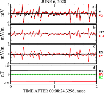
Figure 6. Time domain structures observed at a time when BZ ∼ 0 so the full electric field and background magnetic field were measured in the X−Y plane.
Download figure:
Standard image High-resolution image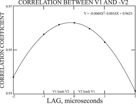
Figure 7. Measured ∼100 ns time lag between observation of V1 and V2 of Figure 6, which shows that the speed of the time domain structure was the order of the electron thermal speed.
Download figure:
Standard image High-resolution imageFigure 8 illustrates the orientation of the moving time domain structures in the magnetic field. In Figure 6(d), the magnetic field was largely along the −Y direction, as shown in Figure 8. Because the direction from V1 to V2 was largely along the −Y direction (see Figure 1 of Mozer et al. 2020a), the time domain structures moved generally in the −Y direction, as illustrated in Figure 8. The EY electric field of Figure 6(c) was first negative and then positive as shown in Figure 8. Thus, the electric field vectors in Figure 8 pointed outward from the time domain structure to produce a positive potential. This is the final proof that the time domain structures were electron holes. We note that the electron holes propagated parallel to the local magnetic field that was generally sunward. Electron holes have been studied extensively in theory, the magnetosphere, and in the lab (Mozer et al. 2015, 2018; Hutchinson 2017).
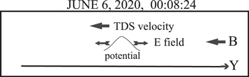
Figure 8. Geometry of the magnetic field, the electron hole velocity, and its electric field, showing that the electron hole had a positive potential and moved sunward.
Download figure:
Standard image High-resolution imageThe electron hole of Figure 6 traveled at 8000 km s−1 and the FWHM of its potential was about 30 μs. Thus, its size was about 240 m, which is about 60 Debye lengths. The peak potential in these structures was about 4 mV m−1 times 240 m, or ∼1 V.
Figures 9 and 10 present two additional examples of electron holes having the same properties as those discussed for the event of Figure 6. It is noted that the three electron hole events, as well as the earlier discussed ion hole event, were observed inside or at boundaries of magnetic field switchbacks because BZ was not dominant.
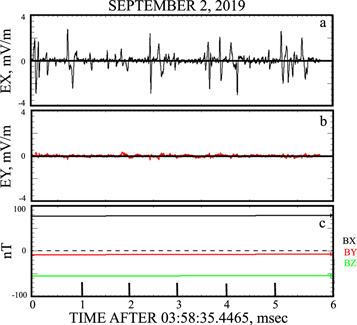
Figure 9. Example of electron holes that moved sunward.
Download figure:
Standard image High-resolution image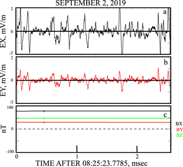
Figure 10. Another example of electron holes that moved sunward.
Download figure:
Standard image High-resolution imageThe electron holes of Figure 6 were associated with modifications of the plasma electrons, as illustrated by the pitch angle distributions of 23–132 eV electrons plotted in Figure 11. At the time of the electron holes (2 s into the plot), the intensity of 36–85 eV electrons at small pitch angles increased. This was a common feature of the holes in the other figures, as shown by the pitch angle distributions of 36–69 eV electrons in Figure 12. The electron holes associated with panels (a), (c), and (d) moved sunward, and they all exhibited the increased electron fluxes of sunward-moving halo electrons. The ion holes of panel (b) were also moving sunward but there was little or no electron flux increase at small pitch angles relative to quiescent conditions.
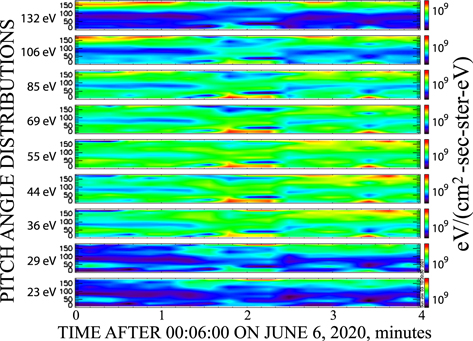
Figure 11. Electron pitch angle distributions during the electron hole observations of Figure 6, which show an increase of sunward-moving 23–85 eV electrons during the electron hole observations.
Download figure:
Standard image High-resolution image
Figure 12. Pitch angle distributions of 36–69 eV electrons during the electron hole events of Figures 6, 9, and 10 as well as the ion hole event of Figure 3. All events were sunward moving, and the three electron hole events all showed an enhancement of sunward-moving halo electrons at the times of the events.
Download figure:
Standard image High-resolution image
5. Discussion: Nonlinear Ion Acoustic Waves
Ion -acoustic waves can be produced by several different instabilities, including ion–ion and ion–electron acoustic instabilities (Gurnett et al. 1979; Gary & Omidi 1987) and Buneman-type instabilities (Buneman 1958; Büchner & Elkina 2006). In the nonlinear stage, the ion-acoustic waves can steepen, resulting in distortion of the electric field waveform and generation of second and higher harmonics of the fundamental wave frequency (Montgomery 1967; Temerin et al. 1979; Lee & Kan 1981; Vasko et al. 2018a). The nonlinear ion-acoustic wave presented in Figure 1 is similar to that expected for steepened ion-acoustic waves, i.e., the waveform consists of unipolar-like electric field spikes formed due to a purely fluid effect that is the steepening of the electrostatic potential.
Ion-acoustic waves can resonate with low-energy electrons via the Landau resonance, which is the only possible resonance for waves polarized parallel to the local magnetic field. The energies of these electrons will be below a few eV, because the velocities of the waves in the plasma rest frame are a few hundred km m−1. The nonlinear ion-acoustic waves have power at the second harmonic and therefore the resonant energies can be a factor of 4 larger, but still below ∼10 eV.
6. Discussion: Ion and Electron Holes
Observations have been presented of more or less sinusoidal ion-acoustic waves followed by a series of bipolar electric field structures interpreted as ion holes. Numerous simulations have shown that such purely kinetic solitary waves are produced in a nonlinear stage of ion-streaming instabilities such as, for example, ion–ion instability (e.g., Goldman et al. 2003; Guio et al. 2003).
Electron holes are produced in the nonlinear stage of various electron-streaming instabilities. The observed electron holes propagate sunward with velocities of ∼8000 ± 4000 km m−1, which is about twice the electron thermal velocity. The most likely source of these electron holes are electron beams at energies of about 50–500 eV propagating sunward and driving an electron-beam instability (e.g., Omura et al. 1996; Pommois et al. 2017; Lotekar et al. 2020). In that case, the fluxes of electrons propagating in the same direction as the electron holes should be enhanced at the times of the electron hole observations. That is indeed the case as demonstrated in Figures 11 and 12. This is evidence that the electron-streaming instability of the bump-on-tail type most likely produced the observed electron holes. The origin of the sunward beams is not clear, but the most likely scenario is that they were produced in the course of the turbulent cascade at small scales by kinetic Alfvén wave interactions with the ambient plasma (see, e.g., simulations by Génot et al. 2001; An et al. 2021).
The major effect of the electron holes is thermalization of the electron beams (Landau resonant) and transformation of the kinetic energy into thermal energy. Another potential effect is pitch angle scattering of cyclotron resonant electrons, which occurs due to electron scattering by the perpendicular electric field of three-dimensional electron holes (Cranmer & van Ballegooijen 2003; Vasko et al. 2017, 2018b). The efficiency of this mechanism is strongly dependent on ωpe/ωce and the scattering is inefficient in the regime ωpe/ωce ≫ 1, because electron holes are more oblate (perpendicular scale much larger than the parallel scale) in that regime and the perpendicular electric field is small. More precisely, the scaling Eper/Epar ∼ (1+ωpe 2/ωce 2)−0.5 shows that for ωpe/ωce ≫ 1, Eper << Epar and the efficiency of the cyclotron resonance is substantially decreased. Because, in the solar wind, typically ωpe/ωce ∼100, it is expected that the cyclotron resonance is inefficient and the major role of electron holes is to thermalize electron beams via the Landau resonance.
In Figure 6, the electron holes appear to arise from a smaller amplitude wave having a period similar to the width of the electron holes. These are most likely electron-beam modes driven by bump-on-tail instability and transforming into electron holes in the nonlinear stage. A similar effect appears in Figures 9 and 10.
The events in this paper were selected by searching through the electric field data. After making these selections, it was noted that all events occurred inside or at the boundaries of switchbacks in the magnetic field. Thus, they may be associated with the low-frequency Alfvénic turbulence found in such events. The turbulence magnetic field spectrum at sub-ion scales is most likely dominated by kinetic Alfvén waves (e.g., Cranmer & van Ballegooijen 2003; Salem et al. 2012), which can produce ion and electron beams due to their parallel electric fields (e.g., Génot et al. 2001; Valentini et al. 2011, 2014). The electrostatic instabilities associated with these beams can drive ion-acoustic waves and electrostatic beam modes that convert into ion and electron holes in a nonlinear stage (e.g., Omura et al. 1996; Goldman et al. 2003; Guio et al. 2003; Pommois et al. 2017). The Parker Solar Probe measurements indicate that such processes indeed operate around switchback boundaries. In addition, because both electron and ion holes have been observed, we conclude that both electron- and ion-streaming electrostatic instabilities are operating there.
This work was supported by NASA contract NASA-G-80NSSC19K1063. The authors acknowledge the extraordinary contributions of the Parker Solar Probe spacecraft engineering team at the Applied Physics Laboratory at Johns Hopkins University. Our sincere thanks to S. Bale, P. Harvey, K. Goetz, and M. Pulupa for managing the FIELDS science, the spacecraft commanding, and data processing. The work of I.V. was supported by NASA grant 80NSSC18K0646 and National Science Foundation grant No. 2026680. The data used in this paper are publicly available at http://fields.ssl.berkeley.edu/data.