


Abstract
The Stark shift due to blackbody radiation (BBR) is a key obstacle limiting the frequency uncertainty of optical lattice clocks. A well-characterized BBR environment is necessary to know exactly the temperature felt by the cold atoms. In our ytterbium clock, the lattice-trapped atoms are exposed to the thermal radiation of the surrounding vacuum chamber walls and optical windows. Calibrated platinum resistance temperature detectors are used to monitor the vacuum chamber temperature in real time. In order to obtain the effective temperature Teff in the position of the atoms, we perform finite element (FE) analysis to the thermal radiation of the vacuum chamber. Due to the temperature inhomogeneity existing in our vacuum chamber, the limited knowledge of the air convection contributes the largest part of the uncertainty in Teff. For our typical room temperature environment, Teff can be determined with an accuracy level of 160 mK, corresponding to a fractional frequency uncertainty of 5.3 × 10⁻¹⁸ for the BBR Stark shift. Additionally, we use a simple formula to relate Teff to the temperatures at the monitored points, which allows us to know the value of Teff without using FE analysis, and thus enables the real-time correction to the BBR Stark shift.
Export citation and abstract BibTeX RIS

Original content from this work may be used under the terms of the Creative Commons Attribution 4.0 licence. Any further distribution of this work must maintain attribution to the author(s) and the title of the work, journal citation and DOI.
1. Introduction
Optical clocks based on lattice-trapped neutral atoms or single trapped ions have reached frequency uncertainty levels in the 10−18 range [1–6], surpassing the cesium primary frequency standard by orders of magnitude. The superior performance of optical clocks has motivated serious considerations of a future redefinition of the SI second in terms of an optical transition. In fact, the International Committee for Weights and Measures has defined five milestones toward such a redefinition [7]. Absolute frequency measurements of the 87Sr and 171Yb clock transitions have achieved an uncertainty level at low 10−16, limited only by the performance of Cs fountain clocks. Combined with optical frequency ratios measured via direct optical comparison, the frequency measurements of 87Sr, 171Yb and Cs clocks have realized a loop closure [8], consistent at the uncertainty limit of the current realization of SI second. In parallel, much efforts have been devoted to incorporate optical frequency standards into existing time scales [9–15]. Besides time and frequency metrology, ultra-precise optical clocks have found wide applications for relativistic geodesy [16, 17], measurement of possible variations of fundamental physical constants [18–20], dark matter detection [21–24] and gravitational wave astronomy [25].
For optical lattice clocks based on Sr or Yb atoms, blackbody radiation (BBR) can induce a Hz-level Stark shift at room temperature. The uncertainty from this frequency shift usually dominates the uncertainty budget table of a clock. Well controlled and characterized BBR environment is important for improving both the frequency uncertainty and long-term stability. Since it scales quarticly with the absolute temperature T of the environment, the BBR Stark shift of the clock transition will be reduced if the atoms are interrogated in a cold environment. Equipped with a cryogenic chamber, Sr clocks at RIKEN that transport ultracold atoms into the cryogenic environment for spectroscopic interrogation reached an uncertainty level of 9 × 10⁻¹⁹ for BBR Stark shift [4]. Other strategies have been used to improve BBR shift uncertainty for clocks operating at room temperature. The technique of in situ temperature monitoring has enabled accurate determination of the BBR temperature felt by the atoms in a Sr clock at JILA [2]. An alternative strategy has been developed for the Yb clocks at NIST. An in-vacuum BBR shield enclosing the atoms ensures a uniform, well characterized BBR environment, yielding a BBR shift uncertainty of the order of 10−19 [26].
We have built an 171Yb optical lattice clock, and its closed-loop operation was reported elsewhere [27]. Since we did not place a BBR shield inside the vacuum, the Yb atoms are exposed to thermal radiation of the vacuum chamber while the whole apparatus sits in the air of the laboratory. For an lattice clock operated at room temperature environment like ours, the BBR temperature can be estimated with uncertainties at low kelvin level [28–30] or sub-kelvin level [31, 32], depending on the degree of temperature homogeneity. We have performed a finite element (FE) analysis to the BBR environment of the ultracold Yb atoms in our setup. The main heat source and the air convection around the main vacuum chamber have also been taken into consideration. We show that the effective temperature felt by the atoms can be determined to an accuracy level better than 200 mK, despite of the temperature inhomogeneity on the vacuum chamber. Our Yb clock can thus achieve a BBR shift uncertainty below 10−17.
The paper is organized as follows. In section 2, the experimental setup is described. In section 3, we introduce the FE analysis for the BBR radiation of our vacuum chamber, and give the effective solid angles of surrounding vacuum parts. We then describe the FE calculation of the effective temperature in section 4. In section 5, we discuss various factors that contribute to the uncertainty budget of the effective temperature. In section 6, we present a simple method to estimate the effective temperature with a good accuracy. Finally, we conclude and discuss our results.
2. Experimental setup
The details of our experimental setup have been described elsewhere [33, 34]. Our vacuum chamber enclosing the ultracold atoms are assembled from commercial stainless-steel vacuum parts and Conflat silica viewports (see figure 1). Thirteen platinum RTDs distributed throughout the external surface provide an real-time measure of the chamber's absolute temperature. One additional RTD is place near the vacuum system to monitor the room temperature. All these RTDs (Omega; PT100) have been calibrated at National Institute of Metrology of China. For a sense current of 1 mA through an RTD, the self-heating reaches a steady-state value of ∼6 mK with a time constant of about 2 s. In practice, the sense current is applied to each RTD only for a short time of 1 s when temperature measurement is required. Therefore, the self-heating effect is actually less than 3 mK. The chamber is connected to the Zeeman slower through a stainless-steel tube. Local heat sources which affect the chamber's temperature include a pair of coils for MOT, Zeeman slower coils and an atomic oven. The MOT coils are water cooled, and its mount is very close to the main chamber, as shown in figure 1. Despite the water cooling, the coil mount surfaces close to the main chamber are still noticeably hotter than the chamber body. So the MOT coils dominate the heating effect although there is no mechanical contact between them. The readout of the RTDs shows a non-uniform temperature distribution, and the maximum temperature difference is as large as ∼2 K.
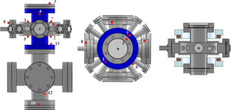
Figure 1. The main vacuum chamber accommodating the ytterbium atoms. The left and middle diagrams are the side and top view, respectively. The right diagram is a central section of the main chamber and the magneto-optical trap (MOT) coil mount, where the brown shaded areas depict the copper coils. The chamber has thirteen fused-silica optical windows, including eight 1.33-in. CF windows, three 2.75-in. CF windows and two 4.5-in. CF windows. Solid squares depict the thirteen resistance temperature detectors (RTDs) attached to the external surface of the stainless steel chamber. The gray solid circle marks the location of the trapped atoms, while the blue area marks the external surfaces covered by the MOT coils. The Zeeman-slowed thermal atomic beam enters the chamber through the tube on the left (truncated for display purposes).
Download figure:
Standard image High-resolution imageAs the atoms are illuminated by the thermal radiation of the chamber, they feel a temperature which depends upon the local field energy density u in the form of cu/(4σ), where c is the speed of light and σ is the Stephan–Boltzmann constant. Due to temperature inhomogeneity, the thermal radiation of the chamber deviates from an ideal BBR environment. To account for departures from an isothermal environment, each radiating surface can be described by its own temperature and effective solid angle viewed by the atoms. The effective radiation temperature at the position of the atoms, Teff, can thus be expressed in terms of effective solid angles of the surrounding surfaces [26]:

where  and Ti
are the effective solid angle and the temperature of surface i, respectively, and i runs over all enclosure surfaces. Similar to geometric solid angles, effective solid angles satisfy the normalization condition
and Ti
are the effective solid angle and the temperature of surface i, respectively, and i runs over all enclosure surfaces. Similar to geometric solid angles, effective solid angles satisfy the normalization condition  . Apparently,
  represents the weight of the corresponding surface i in the calculation of Teff. Different from geometric solid angles, an effective solid angle depends on the geometry and emissivity of all other surfaces. Only in the limit of a completely black environment,
  reduces to the geometric solid angle Ωi
.
reduces to the geometric solid angle Ωi
.
As shown in the work mentioned above [26], both the effective temperature and effective solid angles can be obtained from a steady-state thermal analysis based on FE method. Such an analysis can take into account all sorts of heat transfers, including thermal radiation, heat conductivity, as well as convection of the air. We reconstruct in SolidWorks the mechanical structure of the vacuum chamber, and then load it to ANSYS steady-state thermal [35] where the simulation is carried out. All the internal surfaces of the chamber and optical windows are treated as opaque, diffuse graybody surfaces with temperature-independent emissivities. On the walls of the chamber, there are two apertures that provide access to the Zeeman slower and the ion pump, respectively. We treat each aperture as a disk-shaped blackbody surface with the same size, which is reasonable because each aperture opens up to a large volume of the closed vacuum system. In our model, ytterbium atoms are replaced by a small blackbody sphere with a diameter of 2 mm, which acts as a probe. When the entire system has reached thermal equilibrium, the temperature of the probe represents the effective temperature felt by the atoms.
3. Effective solid angles of the surrounding vacuum parts
Effective solid angle is only related to thermal radiation properties of the surrounding surfaces. Therefore, in the calculation of  , we do not need to consider the air convection and heat conductivity for the chamber body. Noting that the walls of our vacuum chamber and optical windows have absolute temperatures very close to the room temperature, we can use effective solid angles in the case of uniform temperature distribution to characterize the realistic system. The expression of
  can be derived from equation (1), and written as
In fact,  can be simplified to ∂Teff/∂Ti
because of Teff/Ti
≈ 1. In our model, the vacuum chamber is set to a steady state in which the whole chamber holds an identical temperature except the vacuum component i of interest. We add a small gap of 0.1 mm between component i and the chamber body in order to avoid mechanical contact. Doing so, we can set a temperature Ti
for component i that may be different from the chamber temperature. The value of Ti
is chosen from a narrow range around the chamber temperature. Then Teff is calculated for each given Ti
. Finally, we deduce the value of
can be simplified to ∂Teff/∂Ti
because of Teff/Ti
≈ 1. In our model, the vacuum chamber is set to a steady state in which the whole chamber holds an identical temperature except the vacuum component i of interest. We add a small gap of 0.1 mm between component i and the chamber body in order to avoid mechanical contact. Doing so, we can set a temperature Ti
for component i that may be different from the chamber temperature. The value of Ti
is chosen from a narrow range around the chamber temperature. Then Teff is calculated for each given Ti
. Finally, we deduce the value of  from the slope of the Teff(Ti
) curve.
from the slope of the Teff(Ti
) curve.
In table 1 we have listed the effective solid angles for all the vacuum parts. In the calculation typical emissivity values have been adopted for different surface materials. For comparison, geometric solid angles have also been calculated using unit-emissivity (ɛ = 1) for all surfaces. As predicted, the effective solid angle of a vacuum part is not equal to its geometric solid angle. Particularly for optical windows, effective solid angles are much larger than the corresponding geometric solid angles due to the low emissivity of stainless steel walls. The total effective solid angle of the thirteen optical windows,  , is about 17.7% of the full solid angle.
Table 1. Effective and geometric solid angles of the enclosure surfaces of our vacuum chamber. In the calculation, the emissivities of fused-silica windows and stainless steel are set to be 0.94 and 0.4, respectively.
| Vacuum parts |

|

|
|---|---|---|
| Fused-silica windows | ||
| 1.33'' CF ( × 8) | 0.012 26 | 0.010 63 |
| 2.75'' CF ( × 3) | 0.041 82 | 0.023 68 |
| 4.5'' CF (top) | 0.118 68 | 0.041 94 |
| 4.5'' CF (bottom) | 0.004 26 | 0.002 79 |
| Subtotal | 0.177 02 | 0.079 04 |
| Stainless steel walls | 0.822 99 | 0.920 96 |
| Total | 1.000 01 | 1.000 00 |
In our model, all radiation surfaces have been assumed to be opaque to the room-temperature BBR which has a broad infrared spectrum peaked at nearly 10 μm. In fact, a fused silica window is not completely opaque, and a small fraction of thermal radiations can pass through it. According to the reported transmittance of fused silica over the wavelength region above 2 μm [36], the transmittance of our 3 mm thick fused silica windows is estimated to be t = 1.4%. The small residual transmission has no significant effect on the effective temperature Teff for the following reasons: First, the optical windows cover a rather small effective solid angle compared to the stainless steel walls. Secondly, since the chamber's temperature is pretty close to the room temperature, the incoming and outgoing thermal radiations are nearly balanced. Explicitly, as viewed by the atoms, the residual thermal radiation imbalance should cause a small change of Teff which can be written as
For a temperature difference as large as 1 K between Troom and Teff,  is only 2.5 mK. It is clear that the opaque gray body assumption is reasonable in the calculation of Teff, although a small correction must be considered.
4. Calculation of the effective temperature
Since the ambient temperature for our optical clock changes very slowly, the heat transfer of the vacuum chamber is actually in a steady state at a given time. In our FE analysis program, the thirteen RTDs attached to the chamber are modeled as small stainless steel disks with a diameter of 2 mm and a thickness of 1 mm. Temperatures of all the fourteen RDTs, including the one used to monitor the room temperature, are fixed to their measured values in the simulation. Since convection of the air is also considered in our program, the room temperature and convection heat transfer coefficients around the external surfaces are required as input parameters. As the dominating heat source, the MOT coils affect the temperature distribution of the main chamber through its thermal radiations. This effect cannot be totally reflected by the nearby temperature sensors. Therefore, we include also the MOT coils in the FE analysis for the completeness of our model. For the normal power dissipation of MOT coils, the coil mount surfaces close to the chamber reach a temperature of 309 K, about 11 K higher than that of the chamber. The coil mount is made of aluminum alloy, and its surfaces are polished. Its emissivity is set to be 0.1 in the calculation.
Initially the vacuum chamber and the probe are assigned a uniform temperature value that is close to the room temperature. As the simulation proceeds, the temperature distribution of the vacuum chamber will approach a steady state, while the effective temperature Teff converges to a fixed value. The steady-state temperature distribution, as well as the corresponding Teff, are thus obtained after sufficient steps of iterations.
A source of trouble is the lack of knowledge about coefficients of heat convection. Part of the external surfaces of our chamber (the blue area in figure 1) is covered by the closely located coil mount, and the air convection in this area is weakened to some extent. In contrast, other part of external surfaces are exposed to a large volume of the air, which facilitates the air convection. Accordingly, we assign a larger coefficient of heat convection, h1, to the open surfaces, and a smaller one, h2, to the covered surfaces. The following procedure is used to determine the optimum values of h1 and h2. Among the thirteen RTDs on the chamber, we use eleven of them to calculate the steady-state temperature distribution, i.e., the other two RTDs are spare ones and their measured temperature values are ignored by the FE program. By adjusting h1 and h2, we let the calculated temperature values on positions of the two spare RTDs match well with the measured values, and a pair of optimum values of h1 and h2 is then obtained. Choosing different RTDs as the two spare ones, we repeat the calculation, and obtain a new pair of optimum values. The averaging for four times repeated calculation yields h1 = 3.3 W (m2K)−1 and h2 = 0.4 W (m2K)−1. We have adopted this pair of values in the calculation of Teff. Note that h1 here is pretty close to the recommended value for natural convection in air (4 W (m2K)−1) [37].
Figure 2 displays a typical steady-state temperature distribution of the vacuum chamber (MOT coils are not shown for clarity). The CF flanges connected to the Zeeman slower are the hottest vacuum parts. Since the main chamber is a bit hotter than the ambient air, the calculated effective temperature is higher than the measured room temperature. A default mesh size of 4 mm has been used in the FE analysis. In order to know the influence of mesh size on Teff, we repeat the calculation with different mesh sizes while keeping all other conditions unchanged (see figure 3). For decreasing mesh size, the effective temperature does not converge to a fixed value, possibly due to the larger error accumulation at smaller mesh sizes. Despite this, the discrepancy in Teff is less than 60 mK. If the Teff value at the mesh size of 4 mm is regarded as the recommended value, then an uncertainty of 47 mK can cover the whole discrepancy range. For comparison, we also calculated Teff in absence of air convection, which is about 150 mK higher than the case with air convection.

Figure 2. Steady-state temperature distribution of the vacuum chamber simulated by our FE program. The calculated effective temperature at this steady state is Teff = 298.006 K. The room temperature measured by an RTD is 297.077 K, while the temperature readings of the 13 RTDs on the chamber are in the range of 296.42 K to 298.52 K. In the calculation the coefficients of heat convection have been set to be h1 = 3.3 W (m2K)−1 and h2 = 0.4 W (m2K)−1, as explained in the text. The emissivities of different materials in the chamber have been set to the same values as in table 1. The thermal conductivities of fused silica window and 304 stainless steel are set to 1.35 W (mK)−1 and 16.2 W (mK)−1, respectively, as specified in [38].
Download figure:
Standard image High-resolution image
Figure 3. The effective temperature versus the mesh size. All parameters except the mesh size are the same as in figure 2 (solid circles). Open circles are the data for the case without air convection (h1 = h2 = 0).
Download figure:
Standard image High-resolution image5. Uncertainty of the effective temperature
As discussed in the previous section, we roughly divided the external surfaces of the vacuum chamber into two regions according to the air convection ability. The coefficients of heat convection were inferred from the self-consistency of temperature distributions. So far we do not know to what extent this simple model has accurately characterized the air convection. In order to estimate the error of Teff due to the lack of knowledge of air convection, we have checked the dependence of Teff on the coefficients of heat convection. To avoid underestimating the error, h1 and h2 are allowed to vary in a wide range. Specifically, both h1 and h2 are varied from 0, the lowest possible value, to a maximum which is three times the optimum value obtained in the previous section. As shown in figure 4, the effective temperature changes with the two convection coefficients. The recommended value of Teff corresponds to the pair of recommended convection coefficients. In the considered range of h1 and h2, the deviation of Teff from its recommended value can be up to 143 mK. We can safely set an uncertainty of 143 mK for Teff to account for the limited knowledge of air convection. This item dominates the uncertainty budget of Teff as shown in table 2.
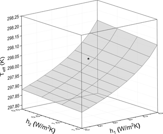
Figure 4. Calculated effective temperature versus the heat convection coefficients in the two regions of the external surface. The solid black dot marks the point corresponding to our recommended values of heat convection coefficients (h1 = 3.3 W (m2K)−1 and h2 = 0.4 W (m2K)−1).
Download figure:
Standard image High-resolution imageTable 2. Effective temperature uncertainty budget for our 171Yb lattice clock.
| Correction | Uncertainty | |
|---|---|---|
| Effects | (mK) | (mK) |
| RTDs temperature measurements | ||
| Resistance calibration | — | 10 |
| Digital multimeter (four-wire) | — | 15 |
| Self heating | — | 3 |
| Air convection | — | 143 |
| Emissivity of windows | — | 1.4 |
| Emissivity of stainless steel | — | 49 |
| MOT coil thermal radiation | — | 3.8 |
| Zeeman slower | 15 | 15 |
| Atomic oven | 7 | 1 |
| Transmission through windows | −2.5 | 2.5 |
| FE analysis error | — | 47 |
| Total | 19.5 | 160 |
The effective temperature is also affected by the two emissivities, ɛSST and ɛwin, which correspond to the stainless steel surfaces and fused-silica windows, respectively. Note that ɛSST depends strongly upon the surface quality of the stainless steel. In reference [38], ɛSST for stainless steel conductors is estimated to be 0.25 by IR camera measurement, while ɛSST for polished stainless steel is measured to be 0.09 in reference [39]. Our vacuum chamber is unpolished, and it has been baked in air before assembling. The surfaces of the chamber show a gray color. Considering the roughness of internal surfaces, we adopted a value of 0.4 for ɛSST in the calculations. In the meantime, considering the strong absorption of the optical windows to the BBR radiation, we adopted a value of 0.94 for ɛwin. We find that Teff increases monotonically with ɛSST (see figure 5). In contrast, Teff is much less sensitive to ɛwin, and it decreases monotonically with ɛwin. We conservatively set an uncertainty range of 0.15 to 0.6 for ɛSST, and then the deviation of Teff from its typical value at ɛSST = 0.4 is less than 49 mK. Similarly, given an uncertainty range of 0.7 to 1.0 for ɛwin, the maximum deviation of Teff is only 1.4 mK.

Figure 5. Dependence of the effective temperature on emissivities of the internal surfaces of the vacuum chamber. Black circles (left scale) and blue circles (right scale) are for the stainless steel walls and the optical windows, respectively. All deviations are relative to the case of the recommended emissivities (ɛSST = 0.4, ɛwin = 0.94). The solid lines are guides to eyes.
Download figure:
Standard image High-resolution imageThe temperature uncertainty of the MOT coil mount should also be considered. Our simulation shows that Teff increases linearly with the mount temperature. An uncertainty of 1 K in the mount temperature leads to an uncertainty of 3.8 mK in Teff. To further understand the thermal radiation effect of the MOT coils mount, we have also calculated Teff when the thermal radiation of the mount is ignored. In this case, Teff is slightly shifted down by 29 mK. This difference is much smaller than the uncertainty caused by the air convection.
The aperture opening up to the Zeeman slower has an effective solid angle of  . In the FE simulation of temperature distribution, the Zeeman slower's flange connected to the vacuum chamber is modeled as a blank flange, which means that the aperture has been replaced by stainless steel disk of the same size. However, the Zeeman slower is hotter than the disk, and its thermal radiation should shift Teff up. This shift,
  , can be expressed in the following form:
where Tslower is the temperature of the Zeeman slower. In fact, the Zeeman slower has an inhomogeneous temperature distribution. If its average temperature is used as the typical temperature, i.e., Tslower = 306 K, we then have to assign a large uncertainty of 8 K to Tslower. The corresponding shift in Teff is  with an uncertainty of 15 mK.
The atomic oven (not shown in figure 1) is further away from the chamber, and it subtends a very small geometric solid angle of 4π × 3.5 × 10−6. The effective solid angle can be approximated by the geometric solid angle because its thermal radiation is almost totally absorbed by the optical window located in the opposite end. In operation state, the oven works at a high temperature of 673 K with an uncertainty of 20 K. Similar to the Zeeman slower, the atomic oven should shift Teff up by an amount of 7 mK with an uncertainty of 1 mK.
The uncertainty budget of the effective temperature has been listed in table 2. The air convection is the dominant contribution, while the second and third largest terms arises from the inaccuracy of stainless steel emissivity and the FE analysis error, respectively. Considering the fact that an effective temperature uncertainty of 1 K sets a fractional frequency uncertainty of 3.3 × 10⁻¹⁷ for an Yb clock [40], the uncertainty level of 160 mK for our vacuum chamber represents a BBR shift uncertainty of 5.3 × 10⁻¹⁸.
6. A method to estimate the effective temperature
During each day the room temperature of our laboratory fluctuates slowly with a peak-to-peak value of ∼1 K. We have calculated the Teff values within 24 hours for discrete times with a half-hour interval. As shown in figure 6, the effective temperature roughly follows the slow fluctuation of room temperature, but with a smaller peak-to-peak variation of about 0.4 K.

Figure 6. Effective temperature calculated from FE program (black open circles) shows slow fluctuation with time. The data points in the first 17 hours have been fitted to formula (2) to determine the coefficients in this formula. Red diamonds represent effective temperatures calculated from formula (2). Solid circles are the temperature differences between these two methods (right scale).
Download figure:
Standard image High-resolution image
Now that the effective temperature changes with time, the optical clock requires real-time corrections to the BBR Stark shift according to the varying Teff. However, frequent FE calculations are time-consuming and inconvenient. We need a faster and simpler method to calculate Teff with sufficient accuracy. Note that the thermal radiation power of a surface element scales as T4, the effective temperature can be expressed as a function of the temperatures at the monitored points:

where Ti
's refer to the temperatures of the fourteen RTDs at a given time, and αi
's are fitting parameters. The data points of Teff obtained by the FE program, here denoted by  for clarity, have been used to determine these fitting parameters. Once the αi
's are set, formula (2) enable us to know the value of Teff without FE analysis any more. We find that the effective temperatures calculated by formula (2), denoted by
for clarity, have been used to determine these fitting parameters. Once the αi
's are set, formula (2) enable us to know the value of Teff without FE analysis any more. We find that the effective temperatures calculated by formula (2), denoted by  , reproduce the corresponding values of
  with an accuracy level better than 0.8 mK (see figure 6).
7. Summary and discussions
For our 171Yb optical clock, the characterization of BBR environment is complicated by the inhomogeneous temperature distribution of the vacuum chamber enclosing the atoms. By using steady-state thermal analysis based on FE method, we have calculated the effective solid angles of the vacuum parts, the steady-state temperature distribution, and the effective temperature Teff. The limited knowledge of air convection is found to be the main source of error for Teff. The total uncertainty of Teff allow us to know the BBR Stark shift with a fractional frequency uncertainty of 5.3 × 10⁻¹⁸. In addition, we have also found that the relation between Teff and temperatures of the RTDs can be well described by a simple formula, which enables real-time thermometry of the BBR environment, and hence real-time corrections to the BBR Stark shift.
Theoretically, adding more RTDs through the external surface of the chamber would allow more accurate simulation of the temperature distribution, and make Teff less sensitive to the heat convection coefficients. This approach, however, will increase the complexity of the apparatus. We are planning to build a new ytterbium optical clock with improved BBR environment. The atoms will be enclosed by an in-vacuum BBR shield, where the temperature homogeneity is expected to be orders of magnitude better.
Acknowledgments
This work is supported by the National Key Research and Development Program of China under Grant No. 2017YFA0304402, by the Natural Science Foundation of China under Grant No. U20A2075, by the Strategic Priority Research Program of the Chinese Academy of Sciences under Grant No. XDB21030100, and in part by the National Natural Science Foundation of China (Grants No. 91636215, No. 11574352, and No. 11803072). We thank Yi-Ge Lin and Zhan-Jun Fang for helpful discussions.