Numerical Simulation and Hydrodynamic Performance Predicting of 2 Two-Dimensional Hydrofoils in Tandem Configuration

Abstract

In this study we investigated the performance of NACA 0012 hydrofoils aligned in tandem using parametric method and Neural Networks. We use the 2D viscous numerical model (STAR-CCM+) to simulate the hydrofoil system. To validate the numerical model, we modeled a single NACA 0012 configuration and compared it to experimental results. Results are found in concordance with the published experimental results. Then two NACA 0012 hydrofoils in tandem configuration were studied in relation to 788 combinations of the following parameters: spacing between two hydrofoils, angle of attack (AOA) of upstream hydrofoil and AOA of downstream hydrofoil. The effects exerted by these three parameters on the hydrodynamic coefficients Lift coefficient ($C_L$), Drag Coefficient ($C_D$) and Lift-Drag Ratio (LDR), are consistent with the behavior of the system. To establish a control system for the hydrofoil craft, a timely analysis of the hydrodynamic system is needed due to the computational resource constraints, analysis of a large combination and time consuming of the three parameters established. To provide a broader and faster way to predict the hydrodynamic performance of two hydrofoils in tandem configuration, an optimal artificial neural network (ANN) was trained using the large combination of three parameters generated from the numerical simulations. Regression analysis of the output of ANN was performed, and the results are consistent with numerical simulation with a correlation coefficient greater than $99.99\%$. The optimized spacing of $6.6c$ are suggested where the system has the lowest $C_D$ while obtaining the highest $C_L$ and LDR. The formula of the ANN was then presented, providing a reliable predicting method of hydrofoils in tandem configuration.

1. Introduction

Hydrofoils are of great interest in designing efficient and high-speed crafts. They can generate enough lift force to raise the main body of the craft when operating in the optimal operation conditions at high speed, decreasing the wetted surface of the craft, and hence reducing a decent amount of resistance or drag. For instance, in [1], a planning craft with a fixed hydrofoil in regular waves was investigated to understand the effects of hydrofoil parameters, such as angle of attack and installation height, on the seakeeping performance. Several hydrofoils under various wavelength and speed conditions were simulated and results of RAOs, resistance and time curve of motion response were predicted and compared. The influence of the speed on the effect of the hydrofoil and the flow field around the planning craft was also investigated and the result showed that with the appropriate arrangement of the hydrofoils, the amplitude of motion response can be significantly reduced.

Analyzing hydrofoils’ performance under different circumstances is one of the crucial subjects in hydrodynamics and has been extensively studied. However, a relatively low number of studies have been performed focusing on analyzing and predicting the hydrodynamic performance of a pair in tandem of hydrofoils.

To better understand the properties of airfoils and hydrofoils, many physical experiments have been done to facilitate numerical modeler to validate their models. For example, a two-dimensional NACA 0012 test program was conducted in the Langley Low-Turbulence Pressure Tunnel, [2] to characterize the airfoil behavior. The lift and drag coefficients of the airfoil were obtained at different angles of attack, Reynold number, and Mach number. The study shows that changes in Mach number affect lift-curve slope and maximum lift coefficient, and changing of these parameters have little effect on either minimum drag or maximum lift-drag ratio. Other well-known 2D lab experiments available for validating numerical models on hydrodynamic parameters such as lift coefficient, drag coefficient, and pressure distribution are The Abbott and von Doenhoff data [3], The Gregory and O’Reilly data [4] and The Ladson tripped data [5]. It is very important for validation of numerical models to consider the experimental range of parameters. Specifically, a collection of NACA 0012 experimental results were discussed by W. J. McCroskey, 1988 [6], observing that experimental drag coefficient levels are greatly affected by tripping the boundary layer at Reynolds numbers in the experimental range. For comparing with “fully turbulent” CFD drag results, tripped experimental data is more appropriate than un-tripped data. In addition, numerical modeling applications have shown that using the turbulent model capability in the commercial CFD software FLUENT 6.0 for hydrofoil turbulent boundary layer separation flow at high Reynold Number, the realizable $\kappa -\epsilon$ model predicts the most precise flow characteristics around the hydrofoils among all the turbulence models. [7].

Recent studies on hydrofoil performance under different working conditions and configuration have been addressed numerically. The free surface wave (wake) generated by the NACA 0015 hydrofoil located close to the free surface was simulated numerically in [8]. The results show that the Volume of Fluid (VOF) method along with realizable $\kappa -\epsilon$ turbulence model can satisfactorily predict wave generated by the flow around a hydrofoil moving near free surface. In addition, when the submergence depth ration goes more than four, the wake is no longer noticeable. In a different study [9], the hydrodynamic performance of a fully passive hydrofoil was analyzed with a 2D fluid-structure interaction model based on the commercial CFD software ANSYS-Fluent. The pitching motion of the hydrofoil was fully induced by the resultant moment caused by the incident water flow. The result shows that with a linear load input acting as a power take-off (PTO) system, the variations in the resultant moment, angular velocity and angle of attack show periodic characteristics. A more complicated flow-separation and vortex-shedding pattern was also observed under the linear load condition. In addition, flow characterization of the wake behind the vortex generator to evaluate the performance of three vortex generator geometries, namely Rectangular VG, Triangular VG, and Symmetrical VG NACA 0012 were analyzed by Gutierrez-Amo, R [10]. Zhen Liu [11] modified the hydrofoil by introducing a custom-designed internal slot, suggesting a significant improvement in performance in lift coefficients, drag coefficients, and lift-drag ratios at high angles of attack.

Presently, hydrofoils are mostly constructed in pairs for craft stability, see Figure 1, where the downstream hydrofoil moves in the wake flow of the upstream, causing a flow-field perturbation around the downstream hydrofoils. Therefore, understanding the interaction between hydrofoils is crucial for craft stability and performance. A numerical parametric study on the interaction between hydrofoils in tandem was provided by Omer Kemal Kinaci [12]. The effects of six different parameters (distance, thickness, chord length, angle of attack, aspect ratio, and tapered wings) were discussed. Kinaci claims that when there is a small distance between the hydrofoils, the flow gets stuck in the gap region to increase the pressure at the trailing edge of the upstream and the leading edge of the downstream hydrofoils. The effect on the interaction vanishes with greater distance. Moreover, the hydrodynamics of two-dimensional tandem hydrofoils travelling below the water surface has been investigated numerically through potential flow theory by G.D. Xu [13], who states that in the design of the hydrofoils boat, the downstream hydrofoils shall be arranged at the zero crossing with an upwash flow. In terms of energy, the “lift augment mode” can be used to save energy. In addition, the wake interactions between two tandem hydrofoils was reviewed by Penglei Ma [14] using numerical investigations to analyze the response of two tandem oscillating hydrofoils. Ma concludes that there is an obvious difference residing in the response of two tandem hydrofoils, owing to the existence of wake interactions. Furthermore, the velocity deficit tends to lower the heaving amplitude and energy harvesting performance of the downstream hydrofoil. In addition, the upstream hydrofoil has a greater time-averaged performance. However, the differences between the responses of two tandem hydrofoils have not a consistent pattern with respect to the spacing of the hydrofoils.

The application of CFD provides a less expensive way to investigate the hydrodynamic performance of a physical model, compared to the elevated construction cost of the model prototype and laboratory test. However, application of CFD needs massive computational resources and some numerical model simulations still are prohibitive. On the other hand, other more simplistic methods based on published data such as analytical data, experimental data, and numerical data can be used to predict the behavior of the physical model or natural phenomenon. For example, there are already several studies in the Ocean Engineering field where Artificial Intelligence tools Neural Networks can be applied to tackle the behavior of the physical model or natural phenomenon reasonably. An example of such application of artificial neural networks (ANN) was presented by Krzysztof Kosowski [15] to investigate the flows parameters in steam turbine cascades. The results proved that ANN could predict the flow parameters reasonably well, and ANN can reduce by several orders of magnitude the time for optimizing these flow parameters. ANN was also coupled with a genetic algorithm by Kamari [16] to optimize the Selig–Donovan 7003 (SD7003) airfoil aerodynamic performance by finding optimum parameters of blowing/suction. Optimization results showed that a significant reduction of the separation zone was achievable. Consequently, perceptible improvements in lift, drag, and aerodynamic performance were achieved. In addition, convolution neural networks (CNNs) were used to combine with Generative adversarial networks (GANs) to directly establish a one-to-one mapping from a parameterized supercritical airfoil to its corresponding transonic flow-field profile over the parametric space [17]. The results showed that this method is a promising tool for the rapid evaluation of detailed aerodynamic performance, which is superior in efficiently and accurately predicting high-dimensional flow field other than low-dimensional aerodynamic characteristics. In other study, Shuyue Wang [18] used ANN to generate new airfoils departing as little as possible from the initial one in the database, which has some aerodynamic features borrowed from other airfoils that constituted the database. The results show that the aerodynamic performance of the new airfoil can be improved to that of the starting points. Moreover, Neural networks were also used to determine the airfoil geometry from a given Cp-distribution by Athar Kharal and Ayman Saleem [19]. ANN was adopted in the active Gurney flap (AGF) flow control technique to enhance the aerodynamic adaption capability of the wind turbine and, thus, achieve an optimal operation in response to fast variations in the incoming wind [20]. Feed-forward back-propagation, generalized regression, and radial basis neural nets were compared in terms of performance and regression statistics, and feed-forward back-propagation neural nets was proven to be more promising in the study. Notably, Hai Chen [21] used convolution neural networks (CNN) to predict the aerodynamic coefficients (pitch-moment, drag, and lift) of NACA 0012 foil. The results showed that the proposed method based on CNN could simultaneously predict all the aerodynamic coefficients listed above of the foil in a very short time and with high accuracy. Similarly, Hashem Nowruzi [22] trained an ANN with the robust databases extracted from CFD simulations of NACA 0012 hydrofoil’s hydrodynamic performance. Based on weight sensitivity analysis in ANN, the Reynolds Number was confirmed to be the most effective factor on the response variable of lift-to-drag ratio (LDR).

In this study, we aim to generate a set of 2D CFD hydrodynamic simulation to obtain the hydrodynamic performance/behavior of a pair of hydrofoil (NACA0012) arranged in tandem and fully submerged under different spacings and AOAs, and thus generate a database of the system performance parameters to train an ANN. NACA 0012 hydrofoil section was selected for its simplified symmetric profile and by the extensive published material allowing us to better understand the underlying physics for further development and investigation. First, the RANS-based CFD approach is used to validate a single hydrofoil model by comparing it with the published experimental data. Numerical model convergence is analyzed, and model resolution is established. Then, the hydrodynamics coefficients and flow regime are obtained numerically for the pair of hydrofoils arranged in tandem for each sample of the set. An optimal artificial neural network (ANN) is obtained using the sample sets generated from the numerical simulation. Additionally, regression analysis of the output of ANN is performed, and the results are compared with the numerical simulation. Furthermore, the formula of the ANN is presented, providing a reliable predicting method of the hydrofoils in tandem configuration.

2. Numerical Simulation

The incompressible viscous flow field around a pair of fully submerged two-dimensional hydrofoils in the tandem configuration is simulated with the STAR-CCM+ based on the Reynolds Averaged Navier–Stokes (RANS). The flow field is assumed to be two-dimensional, incompressible with an infinite water depth and without free surface. The realizable $\kappa -\epsilon$ turbulence model is used for the incompressible viscous flow.

The geometry of the hydrofoils and the incoming velocity of the fluid are set to be Non-dimensional in this study to facilitate comprehension about flow and hydrofoil behavior. The 2D NACA 0012 hydrofoil profile (chord = 1 m) is used in our numerical study.

In this paper, the main objective is to optimize the hydrodynamic performance of the hydrofoil tandem system. In other words, to maximize the lift-to-drag ratio based on hydrofoil spacing and AOAs. It is important to mention that the cavitation effect on the hydrofoils is not considered in this study.

The most important non-dimensional parameter characterizing the flow regimes is the Reynolds number, given by Equation (1).

$$Re=\frac{{\rho }_{\mathrm{water}}Uc}{{\mu }_{\mathrm{water}}}$$

(1)

where c is the foil chord length. Also, other of equal importance is the non-dimensional lift-to-drag ratio (LDR) parameter given by Equation (2).

$$LDR=\frac{L}{D}$$

(2)

where L and D are the lift and drag forces respectively, and $C_L$ and $C_D$ are the lift and drag coefficients as shown in Equations (3) and (4),

$$C_L=\frac{L}{\frac{1}{2}{\rho }_{\mathrm{water}}{U}^{2}l}$$

(3)

$$C_D=\frac{D}{\frac{1}{2}{\rho }_{\mathrm{water}}{U}^{2}l}$$

(4)

Here, l is the characteristic length corresponding to the chord length for the submerged hydrofoil and U is the flow velocity surrounding the hydrofoil system.

For our numerical simulation the STAR-CCM+ computational fluid dynamics program was used under the set of equations and assumptions described above. The second-order implicit stepping in time numerical scheme was used and the results of the unsteady flow were compared to the steady-state results, where the time-averaged flow properties are no longer evolving. The results of both state flow conditions showed a good agreement, therefore, the steady-state condition was adopted in this study.

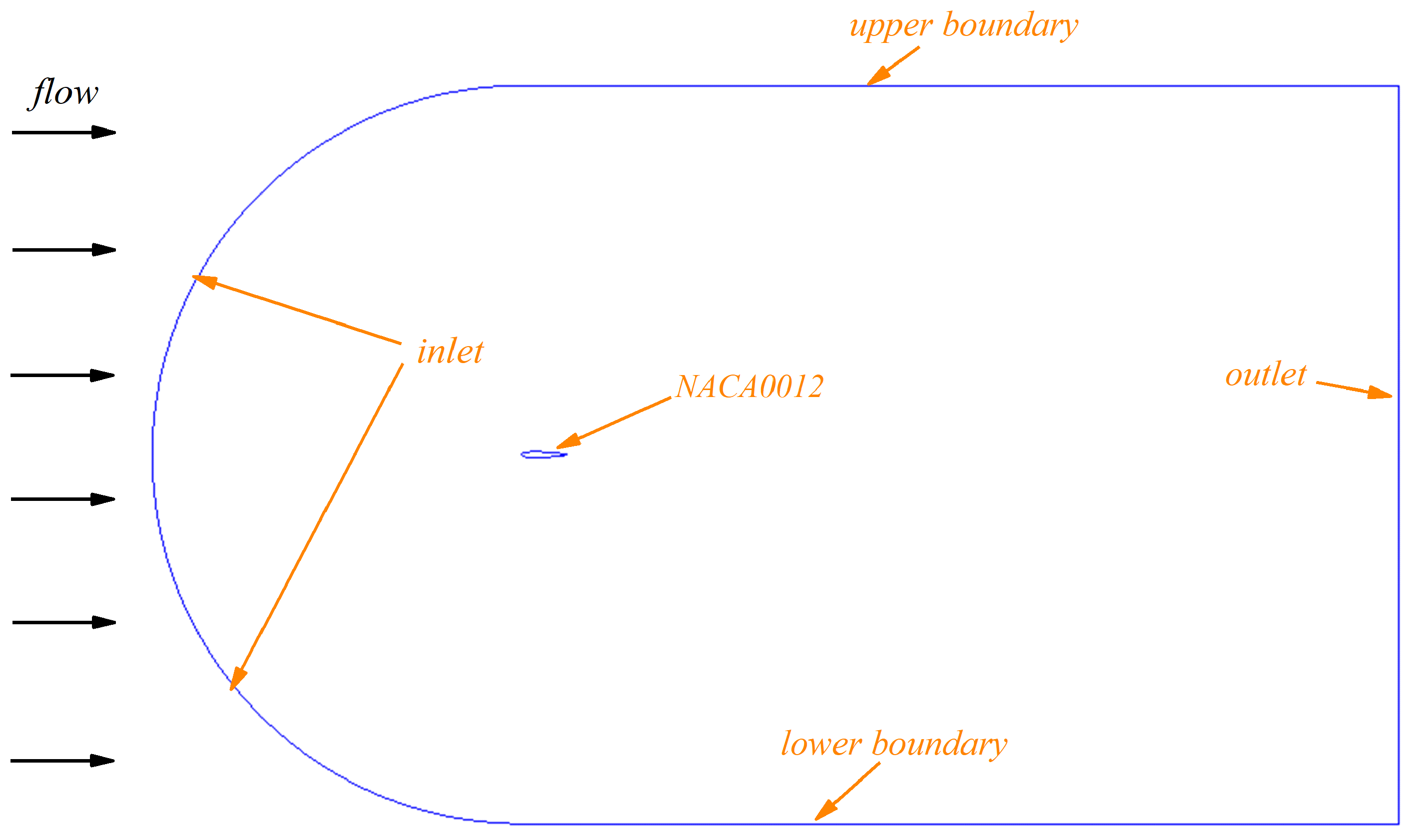
At first, only one hydrofoil was used in the computational model to compare against published experimental data and to validate our numerical setup. The general layout of the computational domain is shown in Figure 1, depicting the inlet and outlet boundaries.

The inlet and outlet boundary conditions are selected to ensure a velocity with a uniform speed at the inlet and a pressure of zero at the outlet. A non-slip wall boundary condition is set at the surface of the NACA0012 hydrofoil. The boundary conditions for the other two surfaces of the computational domain (the upper bound and the lower bound) are set to be symmetric, as shown in

Table 1. Boundary types of computational domain.

Boundary	Boundary Condition
Inlet	Velocity inlet
Outlet	Pressure outlet
Upper boundary	symmetric
Lower boundary	symmetric
Hydrofoil	wall

.

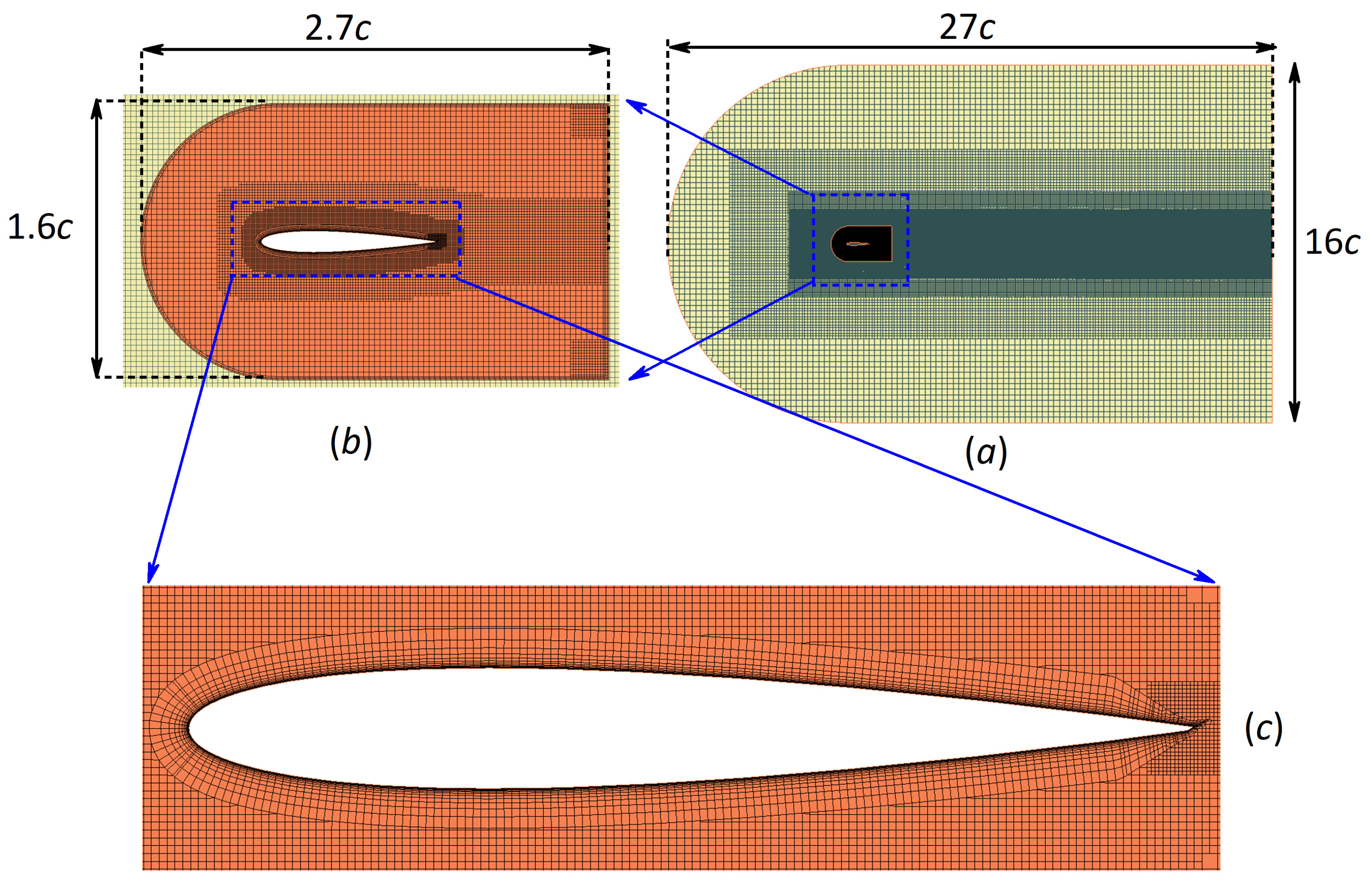
Using the build in generator in the Star-CCM+, the computation domain mesh for this single NACA0012 hydrofoil is generated. As shown in the Figure 2a, a 3D rectangle with a half-sphere inlet was first built as the mesh domain and converted into 2D mesh. The advantage of this mesh compared to the 2D meshing method is that it needs fewer grid faces while still achieving the same computational accuracy. The length and width of the computational domain are set to be 27c and 16c, respectively, where c is the chord length of the hydrofoil. A finer mesh is used around the hydrofoil and the wake zone, while a relatively coarse mesh is used elsewhere. The overset grid technology is used to change the AOA of the hydrofoil as shown in Figure 2b because it can be more convenient to change the hydrofoil’s AOA without regenerating the mesh domain. The length, and the width of the overset grid are $2.7c$ and $1.6c$, respectively. To better analyze the flow field around the NACA 0012, prism layer is adopted closed to the hydrofoil as shown in Figure 2c. The realizable $\kappa -\epsilon$ turbulence model is used in the numerical simulation, and the near-wall flow field is solved by the two-layer all y+ wall treatment. Second-order upwind scheme was adopted for the momentum equation discretization. Second-order upwind scheme was used for the turbulence equation discretization while Gauss-LSQ cell-based scheme was applied for the gradient pressure terms. The pressure-velocity coupling method was set as SIMPLE algorithm. A prism of 25 layers are used around the surface of the hydrofoil with a total thickness of 0.04 m are used around the surface of the hydrofoil. By varying the basic mesh size, three sets of grids (fine, medium, and coarse) are generated for the Verification & Validation procedure. The three density grid sizes are 150 K, 85 K, and 48 K, respectively, and the average refinement ratio $r_G$ is 1.33.

2.1. Mesh Independence Check

To validate mesh independence, three different grid sizes (fine, medium, coarse) were set up and the $C_D$ and $C_L$ are investigated and compared with the experiment results. The numbers of each grid density and their lift and drag coefficients at AOA of $8.1^{\circ }$ are shown in

Table 2. Grid numbers and lift, drag coefficients of each grid Mesh.

Mesh	Total Elements	Lift Coefficient	Drag Coefficient
M1:Fine	151 K	0.8344	0.0160
M2:Medium	85 K	0.8114	0.0147
M3:Coarse	47 K	0.7392	0.0162

as an example.

The CFD simulation uncertainty $U_{SN}$ is divided in four part as shown in Equation (5)

$$U_{SN}=\sqrt{U_G^2+U_T^2+U_I^2+U_P^2}$$

(5)

where the grid uncertainty $U_G$, iterative uncertainty $U_I$, time step uncertainty $U_T$, and another parameter uncertainty $U_P$ need to be solved separately. In this study, only the grid uncertainty $U_G$ needs to be analyzed. [23]

The refinement ratio $r_G$ for 2D problem is defined in Equation (6)

$$r_G={\left(\frac{N_{\mathrm{fine}}}{N_{\mathrm{coarse}}}\right)}^{1/2}$$

(6)

The convergence ratio of numerical simulation can be obtained as follows:

$$R_G=\frac{{\epsilon }_{21}}{{\epsilon }_{32}}=\frac{S_2-S_1}{S_3-S_2}$$

(7)

where $S_1,S_2$, and $S_3$ represent numerical simulation results of the fine, medium, and coarse grid.

The numerical results are in stable state only when $|R_G|<1$. In addition, there are two possible situations as follows:

(i)

$0<R_G<1$, Monotonic Convergence (MC);

(ii)

$R_G<0,\left|R_G\right|<1$, Oscillatory Convergence (OC);

The generalized Richardson extrapolation method is applied to evaluate the numerical calculation accuracy for case (i), where the final numerical calculation grid uncertainty $U_G$ can be calculated using Equation (8)

$$U_G=\left|C_G\frac{{\epsilon }_{21}}{r_G^{P_G}-1}\right|+\left|\left(1-C_G\right)\frac{{\epsilon }_{21}}{r_G^{P_G}-1}\right|$$

(8)

The estimated order of accuracy $P_G$ and asymmetric measurement distance $C_G$ in Equation (8) can be calculated as shown in Equations (9) and (10)

$$P_G=\frac{ln\left|1/R_G\right|}{ln{r}_G}$$

(9)

$$C_G=\frac{r_G^{P_{\mathrm{G}}}-1}{r_G^{p_{EST}}-1}$$

(10)

where $P_{EST}=2$ is the theoretical accuracy.

For the case (ii), the grid uncertainty is calculated by using the maximum value $S_U$ and the minimum value $S_L$ of the oscillation based on the numerical calculation results as shown in Equation (11)

$$U_G=\left|\frac{1}{2}\left(S_U-S_L\right)\right|$$

(11)

The grid uncertainty is shown in

Table 3. Grid uncertainty of the CFD model.

${\mathit{r}}_{\mathit{G}}$	${\mathit{R}}_{\mathit{G}}\left({\mathit{C}}_{\mathit{L}}\right)$	${\mathit{R}}_{\mathit{G}}\left({\mathit{C}}_{\mathit{D}}\right)$	${\mathit{U}}_{\mathit{G}}\left({\mathit{C}}_{\mathit{L}}\right)$	${\mathit{U}}_{\mathit{G}}\left({\mathit{C}}_{\mathit{D}}\right)$
1.33	0.3191 (MC)	−0.8417 (OC)	5.97%	4.44%

. The Lift coefficient of the hydrofoil under AOA of $8.1^{\circ }$ in the 3 grids sets shows a Monotonic Convergence trend while the Drag coefficient shows an Oscillatory Convergence. The calculated grid uncertainty $U_G$ for lift and drag coefficients are all less than six percent of the experimental results.

Furthermore, to validate our CFD numerical model, other studies are investigated. As shown in

Table 4. Comparison of the lift and drag coefficients.

Degree	$\mathit{CFD}-{\mathit{C}}_{\mathit{L}}$	$\mathit{CFD}-{\mathit{C}}_{\mathit{D}}$	$\mathit{EFD}-{\mathit{C}}_{\mathit{L}}$	$\mathit{EFD}-{\mathit{C}}_{\mathit{D}}$	$\mathit{Error}-{\mathit{C}}_{\mathit{L}}$	$\mathit{Error}-{\mathit{C}}_{\mathit{D}}$
1.97	0.2003	0.0101	0.197	0.0108	1.68%	−6.76%
4.14	0.4331	0.0113	0.4219	0.0115	2.66%	−2.18%
5.98	0.6249	0.013	0.6084	0.0134	2.72%	−2.86%
8.1	0.8344	0.016	0.8123	0.0163	2.73%	−2.19%
10.04	1.0093	0.02	0.9789	0.0209	3.11%	−4.66%

, the lift coefficients and drag coefficients of the 2D NACA0012 foil under different angles of attack are calculated and compared with the experimental data. The results also have a good agreement with the experiment data.

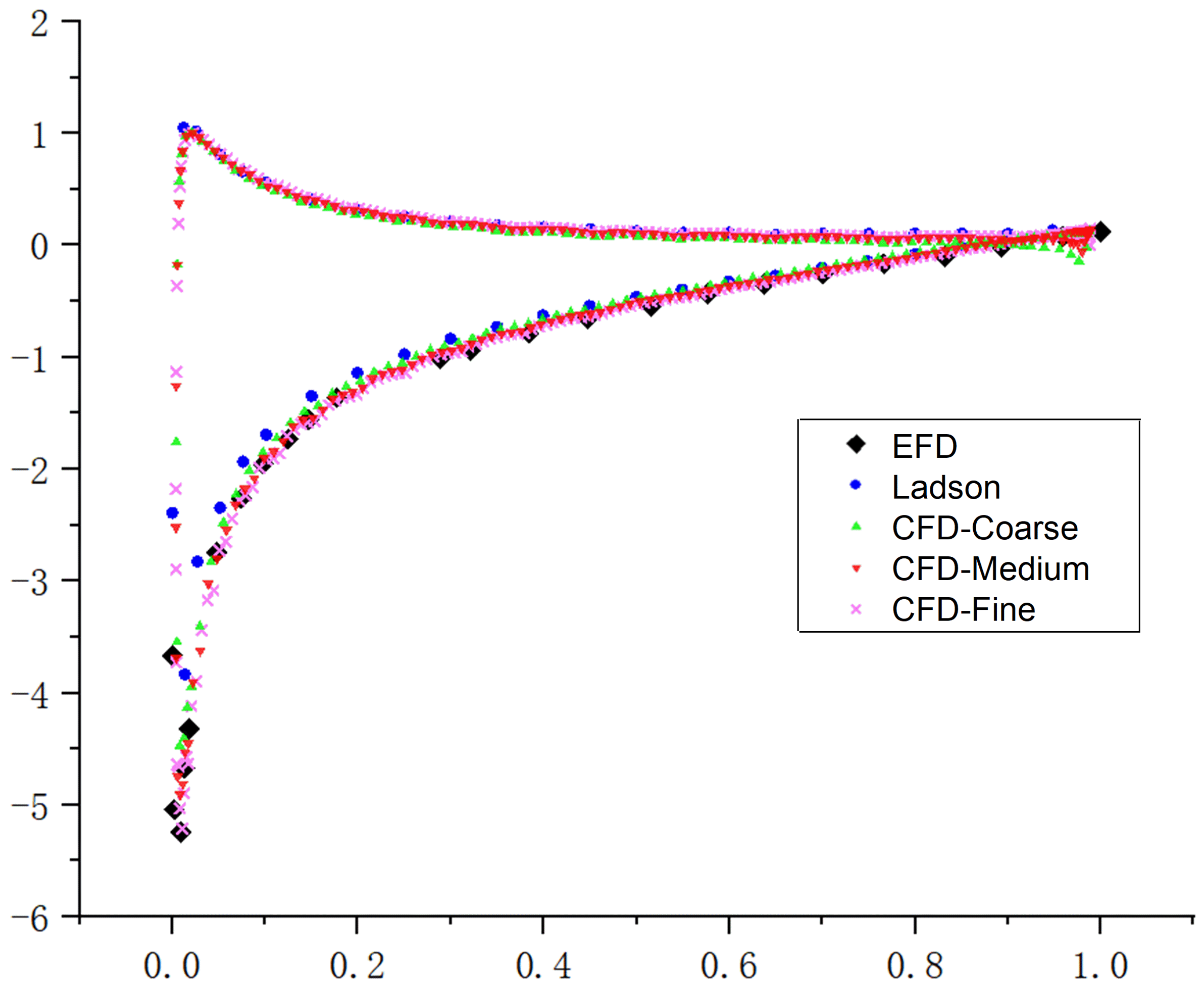
In addition, the pressure distribution on the surface of the hydrofoil of the three grids ( M1, M2, M3) are also investigated and compared with the experiment data, as shown in Figure 3.

The results of the pressure distribution in Figure 3 show that the M 1 with total number of cell $Z=150$ K is an appropriate mesh structure. The face validity of the mesh is checked and $100\%$ of the faces have a face of 1.0, which means that all face normals are properly pointing away from the centroid. The pressure distribution around the hydrofoil matches well with the experiment data.

2.2. Computational Domain of Two Hydrofoils in Tandem Configuration

Using the same method, a computational model of two hydrofoils with tandem configuration was built. The grid structure is shown in Figure 4.

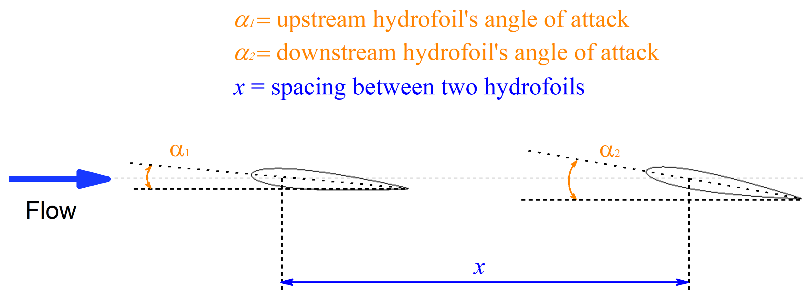
The definitions of the three parameters of the configuration of the tandem arranged hydrofoils ( spacing between two hydrofoils, upstream hydrofoil’s AOA, downstream hydrofoil’s AOA) are shown in Figure 5.

To investigate the effect of these three parameters on the hydrodynamic performance and generate enough data for the Artificial Neural Network(ANN), 788 numerical simulations with the input of different combinations of these three parameters are conducted. The ranges of the three parameters: spacing between two hydrofoils, the upstream hydrofoil’s AOA, and the downstream hydrofoil’s AOA, are set respectively as shown in

Table 5. Range of input variables.

Input Variables	Range	Unites
Spacing between two hydrofoils	2 to 7	chord length
AOA of upstream hydrofoil	0 to 10	Degree
AOA of upstream hydrofoil	0 to 10	Degree

.

The hydrodynamic results obtained by the established computational model can predict reasonable well expected tandem-hydrofoil performance. However, to have a better understanding of how the upstream hydrofoil affects the downstream hydrofoil’s hydrodynamic performance based on an optimal arrangement of the system and thus obtaining an efficient or maximum LDR, more data are needed to be generated to obtain accurate prediction of the hydrofoil system. However, even though the application of CFD simulation provides an inexpensive way to investigate the hydrodynamic performance of a physical model compared to physical model construction and laboratory test associated costs, the application of CFD simulations still need massive computational resources and some complex numerical simulation cases are still prohibitive. Therefore, in the study, we aim to apply a more simplistic method using the numerical data obtained from the hydrofoils performance study that can be used as the basis for the construction of an Artificial Neural Network tool to predict the behavior of the physical model.

3. Artificial Neural Network (ANN) Structures

ANN technology has been applied extensively in Ocean Engineering area. This is due to the ability of ANNs to solve discontinuous and non-linear problems, and to predict the outputs (results) of a complex system based on various selected input parameters with robustness, adaptability, and high accuracy [24]. The BP (back-propagation) Neural Network is used in this study, which is one of the most common type of ANN used for data analysis is the multi-layer perceptron (MLP) networks based on the BP learning algorithm [25].

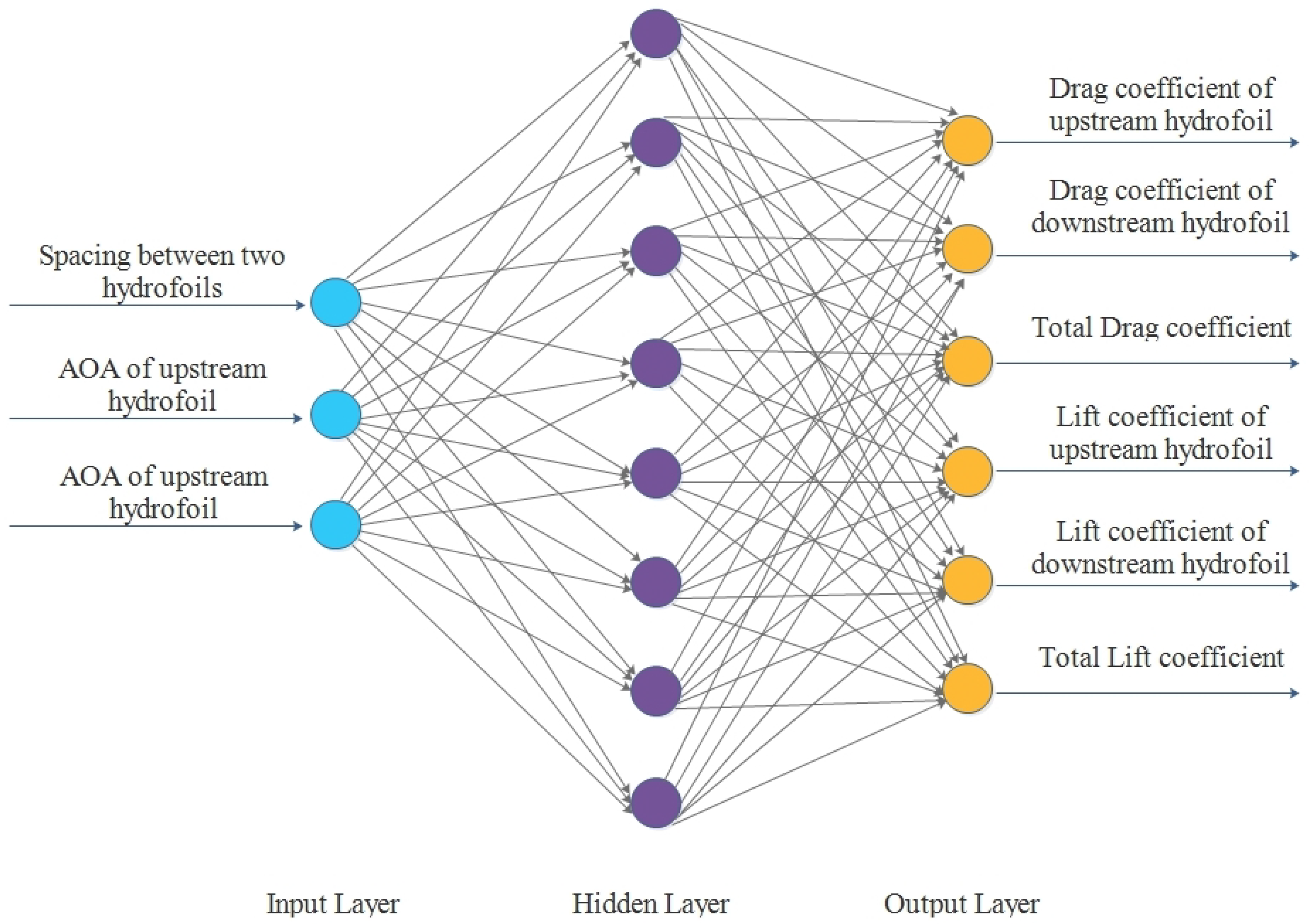
Figure 6 shows the 3-8-6 BP neural network architecture used in this study. The three input layer neurons perform the function of distributing, scaling (if it is necessary), and transfer the three inputs to the processing elements of the next layer. The second layer is the processing or hidden layer, and the eight neurons process the inputs and send their results to the output layer. Finally, the six output-layer neurons represent the six hydrodynamic coefficients predicted by the ANN. The Marquardt–Levenberg algorithm (MLA) was used to optimize of the ANN, stochastic gradient descend method was used for learning procedure.

In the current study, the linear transfer function is used between hidden layer and output layer as shown in Equation (12). $Outpu{t}_1$ to $Outpu{t}_6$ represents the six outputs from the neural network ( downstream hydrofoil’s drag coefficient, upstream hydrofoil’s drag coefficient, total drag coefficient, downstream hydrofoil’s lift coefficient, upstream hydrofoil’s lift coefficient, and total lift coefficient), respectively as shown in Figure 6. ${\omega }_{2ij}$ and $b_{2j}$ are the interconnection weights and bias between the hidden layer and output layer, respectively. In addition, j represents the $jth$ nodes in the hidden layer. $Z_j$ are the values for the eight neurons in the hidden layer. The hyperbolic tangent sigmoid transfer function is selected for neurons between the input and hidden layers, so the value of $Z_j$ can be calculated using Equation (13). Where ${\alpha }_1$, ${\alpha }_2$, and x are the three inputs (AOA of upstream hydrofoil, AOA of downstream hydrofoil, spacing between two hydrofoils), respectively. ${\omega }_{{\alpha }_{1j}}$, ${\omega }_{{\alpha }_{2j}}$, ${\omega }_{x_j}$, and $b_{1j}$ are the interconnection weights for the three inputs listed above and bias between the input layer and hidden layer, respectively.

$$Outpu{t}_i=\sum _{j=1}^8{w}_{2ij}·Z_j+b_{2i},1<i<6,1<j<8$$

(12)

$$\begin{array}{c}\hfill Z_j=\frac{2}{1+exp\left(-2·\left({\alpha }_1·w_{{\alpha }_{1j}}+{\alpha }_2·w_{{\alpha }_{2j}}+x·w_{x_j}+b_{1j}\right)\right)}-1,\\ \hfill 1<j<8,2<x<7,0^{\circ }<{\alpha }_1<{10}^{\circ },0^{\circ }<{\alpha }_2<{10}^{\circ }\end{array}$$

(13)

Mean square errors (MSE) and correlation coefficient R are two error evaluation factors selected to evaluate the quality of the predicted results of the ANN as shown in Equations (14) and (15). N is the number of evidence data and $T_i$ is the reference data (target values). In addition, $O_i$ represents the predicted values using the trained Neural Networks. $\overline{O}$ and $\overline{T}$ are the average values of the reference data and outputs of the Neural Network, respectively. Notably, smaller MSE and a proximity of R to 1 implies a more accurate prediction, referring to a better quality of the Neural Networks.

$$\mathrm{MSE}=\frac{{\sum }_{i=1}^N{\left(O_i-T_i\right)}^2}{N}$$

(14)

$$R=\frac{{\sum }_{i=1}^N\left(O_i-\overline{O}\right)\left(T_i-\overline{T}\right)}{\sqrt{{\sum }_{i=1}^N{\left(O_i-\overline{O}\right)}^2{\sum }_{i=1}^N{\left(T_i-\overline{T}\right)}^2}}$$

(15)

In the present study, 700 out of the 788 CFD simulation results are randomly selected and used as the data base to train the ANN, the other 88 are later used to test the trained ANN. Limited values of considered input-output variables are tabulated in

Table 6. Input and output ranges for ANNs.

Variables	Range	Unites
Input
Spacing between two hydrofoils (x)	2–7	chord-length
AOA of upstream hydrofoil (Alpha 1)	0–10	Degree
AOA of upstream hydrofoil (Alpha 1)	0–10	Degree
output
Total Lift Coefficient (CL)	0–2	Non-dimensional
Total Drag Coefficient (CD)	0.01–0.04	Non-dimensional
Total Lift-to-Drag Ratio (LDR)	0–55	Non-dimensional

. Moreover, to avoid over-fitting, early stopping approach presented by Prechelt [26] is applied in our study by classifying the inputs-outputs of our numerical simulated data in three randomly groups. $70\%$ of the numerical simulated data are used to train the ANN, $15\%$ are used to validate the trained ANN to avoid over-fitting, and the other $15\%$ are used to test the quality of the ANN.

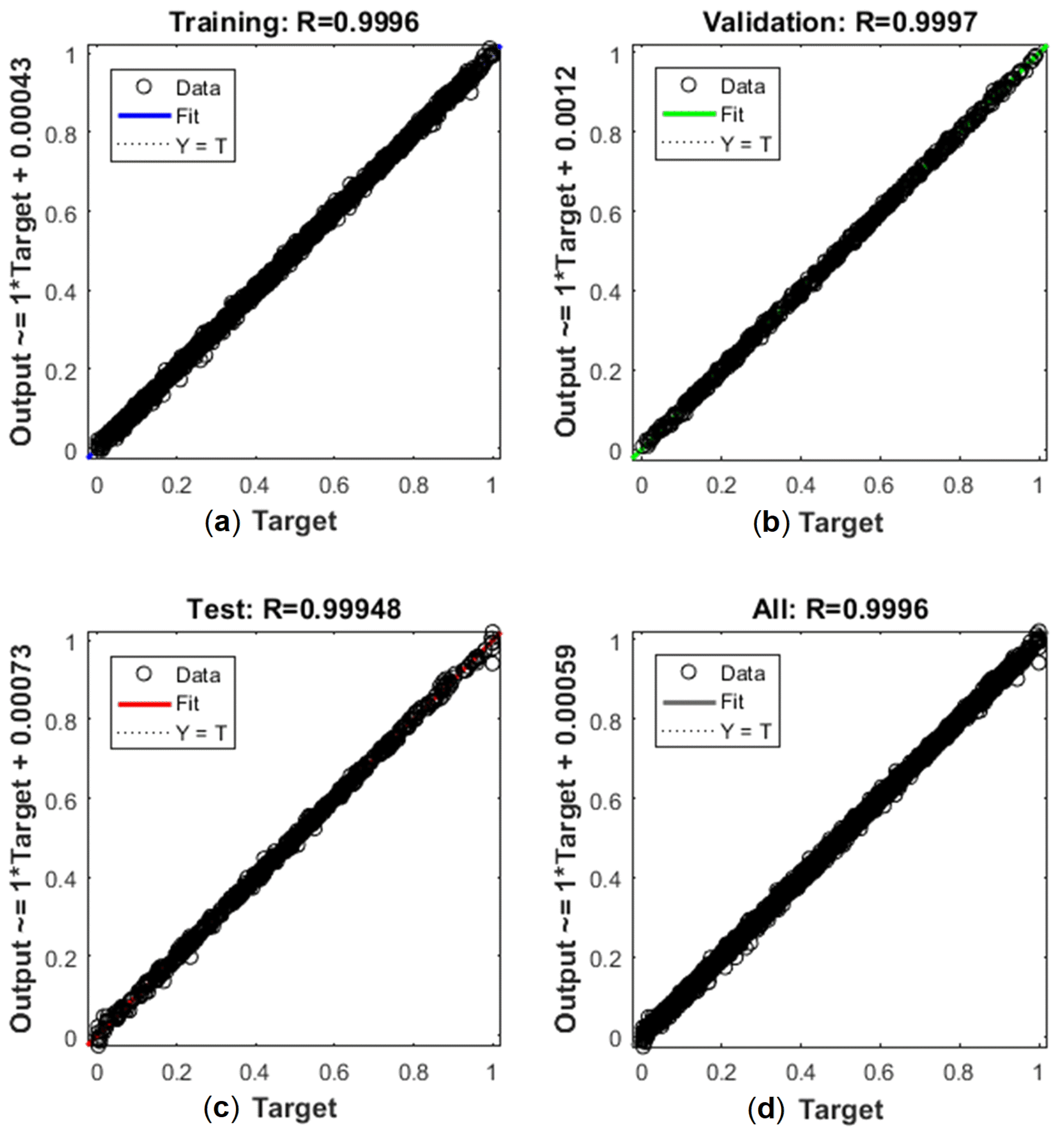
The predicted data are validated with the test data using a linear regression model. In addition, the linear regression analysis are performed for the training sample set, validation sample set, test sample set, and all sample set, respectively, the results are shown in Figure 7.

As shown in Figure 7, the output data from the neural network matches quite well with the targeted data with correlation coefficients $R>99\%$ and $MSE<0.0001$ for all the four sample sets. In addition, the other 88 numerical simulated data are used to test the trained ANN. In addition, the correlation analysis was performed using the same method, with a $R=99.88\%$. Thus, it can be concluded that the selected ANN is able to accurately predict the hydrodynamic performance of the system under different geometric and environmental conditions.

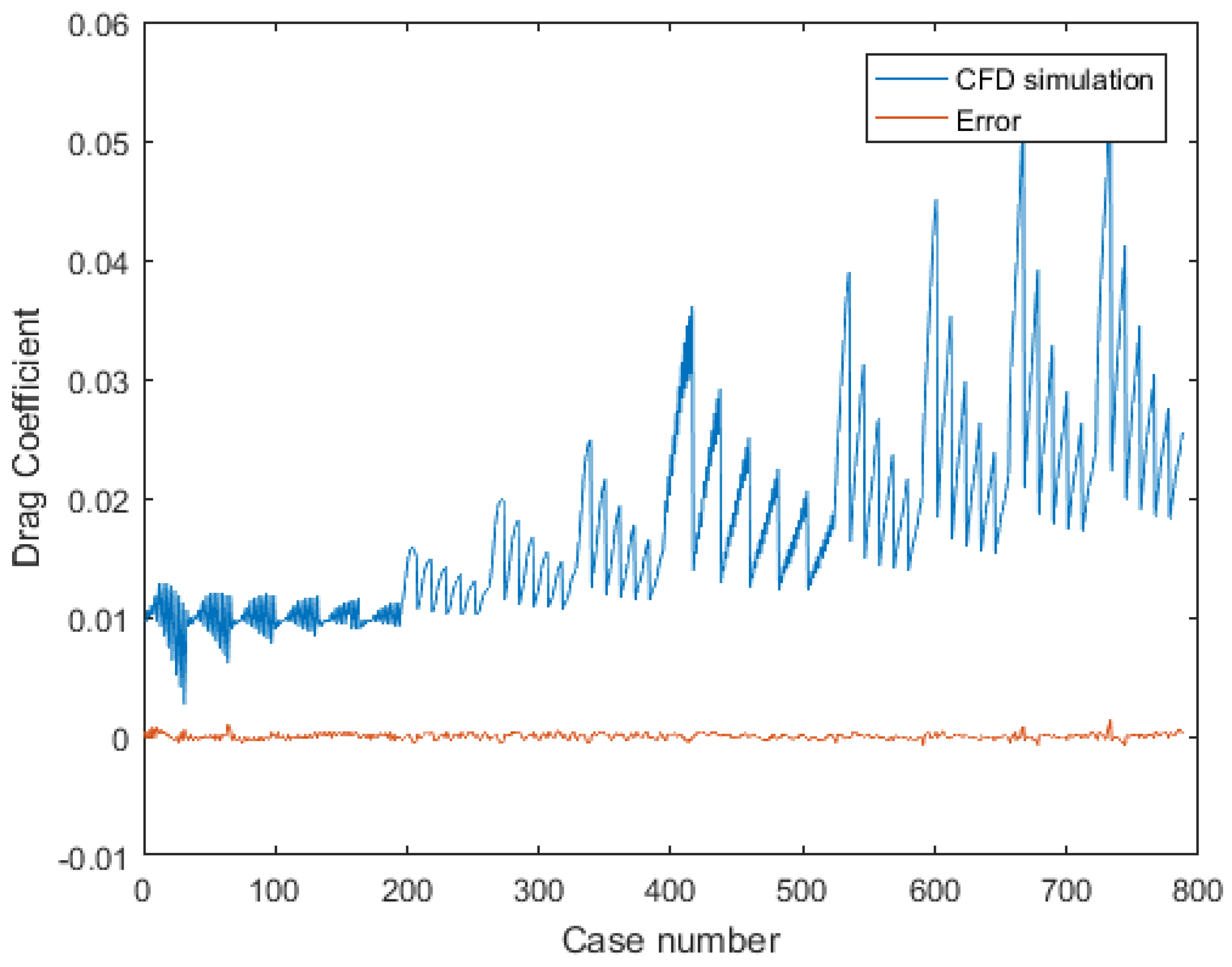
Furthermore, all the 788 CFD simulation data are combined as a whole sample set. In addition, the Neural Network’s prediction for all the 788 cases were compared with the original CFD simulation data. For instance, the results of the CFD simulation and error of the predictions of the ANN of the Drag Coefficient are listed in the Figure 8.

As can be concluded by looking at Figure 8, the differences for all the 788 cases are relatively small compared to the actual CFD simulation results. So, we can conclude that the ANN can be used to substitute the traditional CFD simulation method if the forecast time is limited and still providing a reasonably good prediction.

In addition, to provide a faster and more convenient way to predict the hydrodynamic performance of the system in case the trained ANN is not available. The weights (w) and bias (b) matrix used in the equation according to inputs variables of AOAs and distance presented in Equations (12) and (13) are extracted and tabulated in

Table 7. Constant values of weights and bias for hidden layer.

i	${\mathit{w}}_{\mathit{x}}$	${\mathit{w}}_{{\mathit{\alpha }}_1}$	${\mathit{w}}_{{\mathit{\alpha }}_2}$	${\mathit{b}}_1$
1	1.140	−0.988	−0.657	2.607
2	−0.361	−0.112	0.085	0.0612
3	0.027	0.483	−0.111	−0.659
4	−0.280	0.214	−0.280	0.211
5	0.018	0.099	0.817	−0.930
6	1.016	−0.474	−0.564	2.200
7	0.061	0.092	0.655	0.436
8	0.050	−0.586	−0.031	−0.560

and

Table 8. Constant values of weights and bias for output layer.

j	${\mathit{w}}_{1\mathit{j}}$	${\mathit{w}}_{2\mathit{j}}$	${\mathit{w}}_{3\mathit{j}}$	${\mathit{w}}_{4\mathit{j}}$	${\mathit{w}}_{5\mathit{j}}$	${\mathit{w}}_{6\mathit{j}}$
1	0.605	−1.046	−0.350	−0.292	0.653	0.211
2	−1.501	1.757	−0.467	−0.230	−0.653	−0.523
3	−1.112	2.475	1.522	−0.402	0.633	0.133
4	2.289	−2.473	1.038	0.571	0.996	0.929
5	1.029	−0.592	1.295	0.699	0.291	0.589
6	−2.004	2.827	0.145	0.803	−1.128	−0.185
7	0.977	−0.990	0.548	1.401	0.563	1.169
8	0.694	−0.318	1.002	0.563	−0.734	−0.162
$b_{2_i}$	0.527	0.052	1.529	−0.553	0.259	−0.174

, respectively.

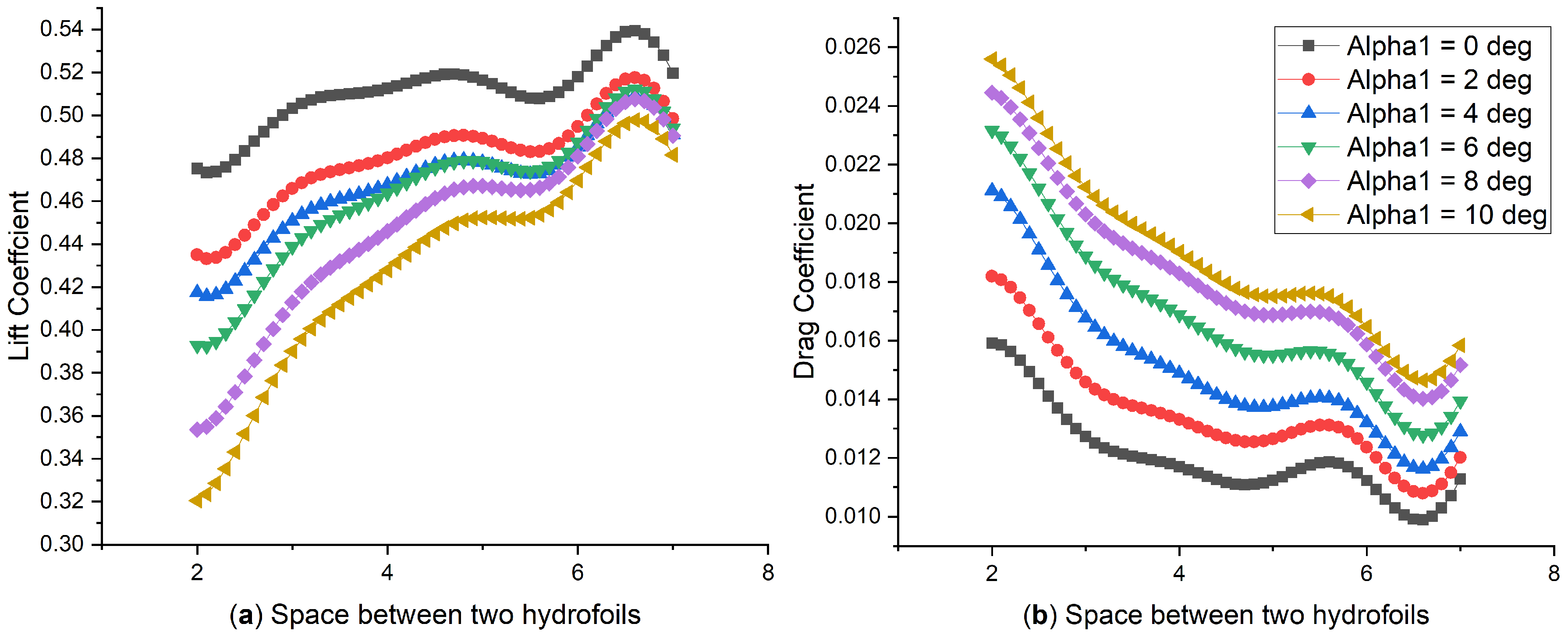
To investigate the effect on the downstream hydrofoil exerted by the upstream hydrofoil at different space between the two hydrofoils. The AOA of downstream hydrofoil is fixed at $5^{\circ }$, the predicted lift coefficient and drag coefficient at different spacing between the two hydrofoils using prediction of the trained Neural network are plotted in Figure 9. Different color represents different AOA of upstream hydrofoil.

As shown in the Figure 9a, there is a critical spacing at 6.6 chord length where the $C_L$ has a local maximum value and the $C_D$ has a local minimum value no matter how much the AOA of the upstream hydrofoil is. When the spacing is smaller than 6.6 chord length, as the downstream hydrofoil gets further away from the upstream hydrofoil, the higher Lift coefficient and lower Drag coefficient will be found at the downstream hydrofoil. Therefore, to let the downstream hydrofoil achieve the highest $LDR$, the downstream hydrofoil should be arranged at $6.6c$ away from the upstream hydrofoil.

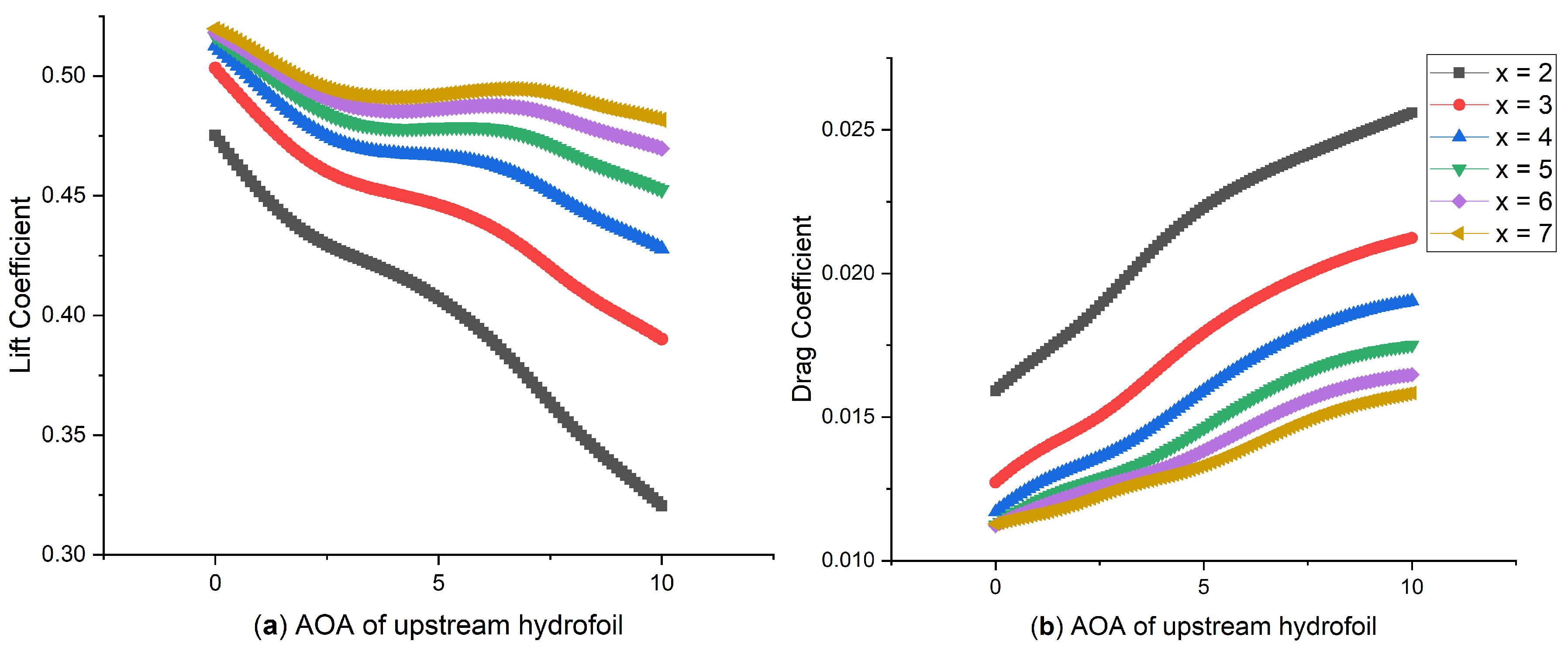
Similarly, the predicted $C_L$ and $C_D$ of the trained Neural network at different AOA of upstream hydrofoil are shown in Figure 10 when the ${\alpha }_1$ is fixed at $5^{\circ }$. Different color represents different spacing between the two hydrofoils. As shown in the Figure 10, as the ${\alpha }_1$ gets larger, the $C_L$ gets lower and the $C_D$ gets higher. In other words, the upstream hydrofoil have a negative effect on the hydrodynamic performance of the downstream hydrofoil. The effect gets less as the spacing between the two hydrofoils gets larger.

4. Conclusions and Future Works

A 2D viscous numerical model based on STAR-CCM+ is generated to simulate the hydrodynamic performance of two NACA 0012 hydrofoils aligned in tandem. The grid independence analysis is validated using the Richardson Extrapolation method. The numerical results are found in concordance with the published experimental results. Then two NACA 0012 hydrofoils in tandem configuration were studied in relation to 788 combinations of x in range of 2c to 7c, AOAs in range of $0^{\circ }$ to ${10}^{\circ }$. In addition, an optimal artificial neural network (ANN) was trained using the sample set generated from the numerical simulation. Regression analysis of the output of ANN was performed, and the results are consistent with numerical solutions. The formula of the trained ANN was then presented, providing a reliable and efficient predicting model of hydrofoils in tandem configuration. The main conclusions are presented below:

1

The computational model using an overset grid technology to change the AOA of the hydrofoil instead of using the traditional method (by changing the vectors of the inlet) is found to show a good capability to simulate the hydrodynamic performance of the system with acceptable accuracy, which could save huge amount of time on the grid generation.

2

The predicted outputs of the optimized ANN matches well with the numerical results with a correlation coefficient greater than $99.99\%$. Showing that the developed methodology used in this study to establish a fast and reliable predicting model can be used in the future for similar system.

3

A critical spacing of 6.6c was found to have the lowest $C_D$ while have highest $C_L$ and LDR for both the downstream hydrofoil and the system. Therefore, to optimize the performance of the system, the downstream hydrofoil should be arranged at $6.6c$ away from the upstream hydrofoil.

4

Mathematical formula for the optimized ANN was achieved, presenting a more efficient way to predict the system’s hydrodynamic performance, which could be further applied to optimize similar systems. In addition, it can also be used to establish the control system of autonomous hydrofoil crafts.

References

- Bi, X.; Shen, H.; Zhou, J.; Su, Y. Numerical analysis of the influence of fixed hydrofoil installation position on seakeeping of the planing craft. Appl. Ocean Res. 2019, 90, 101863. [Google Scholar] [CrossRef]
- Lynch, F.T.; Khodadoust, A. Effects of ice accretions on aircraft aerodynamics. Prog. Aerosp. Sci. 2001, 37, 669–767. [Google Scholar] [CrossRef]
- Abbott, I.H.; Von Doenhoff, A.E. Theory of Wing Sections: Including a Summary of Airfoil Data; Courier Corporation: Chelmsford, MA, USA, 2012. [Google Scholar]
- Gregory, N.; O’reilly, C. Low-Speed Aerodynamic Characteristics of NACA 0012 Aerofoil Section, including the Effects of Upper-Surface Roughness Simulating Hoar Frost. NASA R&M 3726. January 1970. Available online: https://reports.aerade.cranfield.ac.uk/handle/1826.2/3003 (accessed on 22 April 2021).
- Ladson, C.L. Effects of Independent Variation of Mach and Reynolds Numbers on the Low-Speed Aerodynamic Characteristics of the NACA 0012 Airfoil Section; National Aeronautics and Space Administration, Scientific and Technical Information Division: Hampton, VA, USA, 1988; Volume 4074. [Google Scholar]
- McCroskey, W. A Critical Assessment of Wind Tunnel Results for the NACA 0012 Airfoil; Technical Report; National Aeronautics And Space Administration Moffett Field Ca Ames Researchcenter: San Francisco, CA, USA, 1987.
- Mulvany, N.; Tu, J.; Chen, L.; Anderson, B. Assessment of two-equation turbulence modelling for high Reynolds number hydrofoil flows. Int. J. Numer. Methods Fluids 2004, 45, 275–299. [Google Scholar] [CrossRef]
- Karim, M.M.; Prasad, B.; Rahman, N. Numerical simulation of free surface water wave for the flow around NACA 0015 hydrofoil using the volume of fluid (VOF) method. Ocean Eng. 2014, 78, 89–94. [Google Scholar] [CrossRef]
- Liu, Z.; Qu, H.; Shi, H. Numerical study on hydrodynamic performance of a fully passive flow-driven pitching hydrofoil. Ocean Eng. 2019, 177, 70–84. [Google Scholar] [CrossRef]
- Gutierrez-Amo, R.; Fernandez-Gamiz, U.; Errasti, I.; Zulueta, E. Computational modelling of three different sub-boundary layer vortex generators on a flat plate. Energies 2018, 11, 3107. [Google Scholar] [CrossRef] [Green Version]
- Ni, Z.; Dhanak, M.; Su, T.C. Performance of a slotted hydrofoil operating close to a free surface over a range of angles of attack. Ocean Eng. 2019, 188, 106296. [Google Scholar] [CrossRef]
- Kemal, O. A numerical parametric study on hydrofoil interaction in tandem. Int. J. Nav. Archit. Ocean Eng. 2015, 7, 25–40. [Google Scholar]
- Xu, G.; Xu, W.; Duan, W.; Cai, H.; Qi, J. The free surface effects on the hydrodynamics of two-dimensional hydrofoils in tandem. Eng. Anal. Bound. Elem. 2020, 115, 133–141. [Google Scholar] [CrossRef]
- Ma, P.; Wang, Y.; Xie, Y.; Han, J.; Sun, G.; Zhang, J. Effect of wake interaction on the response of two tandem oscillating hydrofoils. Energy Sci. Eng. 2019, 7, 431–442. [Google Scholar] [CrossRef] [Green Version]
- Kosowski, K.; Tucki, K.; Kosowski, A. Application of artificial neural networks in investigations of steam turbine cascades. J. Turbomach. 2010, 132, 014501. [Google Scholar] [CrossRef]
- Kamari, D.; Tadjfar, M.; Madadi, A. Optimization of SD7003 airfoil performance using TBL and CBL at low Reynolds numbers. Aerosp. Sci. Technol. 2018, 79, 199–211. [Google Scholar] [CrossRef]
- Wu, H.; Liu, X.; An, W.; Chen, S.; Lyu, H. A deep learning approach for efficiently and accurately evaluating the flow field of supercritical airfoils. Comput. Fluids 2020, 198, 104393. [Google Scholar] [CrossRef]
- Wang, S.; Sun, G.; Chen, W.; Zhong, Y. Database self-expansion based on artificial neural network: An approach in aircraft design. Aerosp. Sci. Technol. 2018, 72, 77–83. [Google Scholar] [CrossRef]
- Kharal, A.; Saleem, A. Neural networks based airfoil generation for a given Cp using Bezier–PARSEC parameterization. Aerosp. Sci. Technol. 2012, 23, 330–344. [Google Scholar] [CrossRef]
- Saenz-Aguirre, A.; Fernandez-Gamiz, U.; Zulueta, E.; Ulazia, A.; Martinez-Rico, J. Optimal wind turbine operation by artificial neural network-based active gurney flap flow control. Sustainability 2019, 11, 2809. [Google Scholar] [CrossRef] [Green Version]
- Chen, H.; He, L.; Qian, W.; Wang, S. Multiple Aerodynamic Coefficient Prediction of Airfoils Using a Convolutional Neural Network. Symmetry 2020, 12, 544. [Google Scholar] [CrossRef] [Green Version]
- Nowruzi, H.; Ghassemi, H.; Ghiasi, M. Performance predicting of 2D and 3D submerged hydrofoils using CFD and ANNs. J. Mar. Sci. Technol. 2017, 22, 710–733. [Google Scholar] [CrossRef]
- Seo, S.; Song, S.; Park, S. A study on CFD uncertainty analysis and its application to ship resistance performance using open source libraries. J. Soc. Nav. Archit. Korea 2016, 53, 329–335. [Google Scholar] [CrossRef] [Green Version]
- Jiang, J.; Zhang, J.; Yang, G.; Zhang, D.; Zhang, L. Application of back propagation neural network in the classification of high resolution remote sensing image: Take remote sensing image of Beijing for instance. In Proceedings of the 2010 18th International Conference on Geoinformatics, Beijing, China, 18–20 June 2010; pp. 1–6. [Google Scholar]
- Atkinson, P.M.; Tatnall, A.R. Introduction neural networks in remote sensing. Int. J. Remote Sens. 1997, 18, 699–709. [Google Scholar] [CrossRef]
- Prechelt, L. Automatic early stopping using cross validation: Quantifying the criteria. Neural Netw. 1998, 11, 761–767. [Google Scholar] [CrossRef] [Green Version]
Figure 1.
General layout of the computational domain. Arrows indicate location of the inlet and outlet of the computational domain.
Figure 2.
Computational domain and mesh structures. (a) Grid of the computational domain with boundaries. (b) Close-up view of Grid around overset mesh. (c) Close-up view of grid around the hydrofoil.
Figure 3.
Influence of mesh sizing on pressure distribution on the surface of hydrofoil and comparison on experiment data at Re = 3,000,000 and AOA = .
Figure 4.
Computational domain and mesh structures of two NACA0012 hydrofoils in tandem configuration. (a) Grid of the computational domain with boundaries. (b) Close-up view of Grid around overset mesh. (c) Close-up view of grid around the hydrofoil.
Figure 5.
Schematic of the configuration of the tandem arranged hydrofoils.
Figure 6.
Neural network architecture.
Figure 7.
Regression Analysis of the Neural network’s output using (a) training sample set (b) validating sample set (c) testing sample set (d) all sample set.
Figure 8.
Comparison between the prediction from trained ANN and the CFD simulation results.
Figure 9.
The effect of the space between two hydrofoils on the downstream hydrofoil’s (a) Lift Coefficient (b) Drag Coefficient.
Figure 10.
The effect of the AOA of upstream hydrofoil on the downstream hydrofoil’s (a) Lift Coefficient (b) Drag Coefficient.