AGB Winds with Gas-Dust Drift in Stellar Evolution Codes

Abstract

A significant fraction of new metals produced in stars enter the interstellar medium in the form of dust grains. Including dust and wind formation in stellar evolution models of late-stage low- and intermediate-mass stars provides a way to quantify their contribution to the cosmic dust component. In doing so, a correct physical description of dust formation is of course required, but also a reliable prescription for the mass-loss rate. Here, we present an improved model of dust-driven winds to be used in stellar evolution codes and insights from recent detailed numerical simulations of carbon-star winds including drift (decoupling of dust and gas). We also discuss future directions for further improvement.

1. Introduction

Knowledge about how asymptotic giant branch (AGB) stars enrich the interstellar medium (ISM) with metals (i.e., elements heavier than helium) requires understanding of the mechanisms behind their mass loss and how the formation of dust changes throughout their evolution on the AGB. Observational constraints provide important clues, such as the composition of dust produced and abundances of important molecular species for dust growth [1,2,3,4], which allow for testing and calibration of dust-formation models used in stellar evolution codes.

Including wind models and dust formation in stellar evolution codes is normally done in a simplified parametric way [5,6,7]. The most important input parameter is the mass-loss rate for a given set of stellar parameters (e.g., mass, luminosity, effective temperature and atmospheric composition). Getting a handle on the mass-loss rate is, therefore, of fundamental importance. The most common way to prescribe mass loss is by the use of simple formulae obtained from fits to either observations or simulated mass loss, or a combination of both [8,9,10], but any such formula will have trouble capturing all aspects of how mass loss depends on stellar parameters.

Frequency-dependent radiative transfer in wind models has in recent years provided a better basis for creating such mass-loss prescriptions for stellar evolution codes. For carbon stars (C/O > 1), the work by Mattsson et al. [11,12], Mattsson and Höfner [13] and more recently by Mattsson et al. [14], Bladh et al. [15] have provided input data covering a significant part of steller-parameter space. The mass loss of oxygen rich AGB stars (C/O < 1) has been less explored, but Höfner [16], Höfner et al. [17], Bladh et al. [18] have made progress in covering important parts of the stellar-parameter space. However, all these studies have one thing in common: they rely on the assumption that the effect of drift, i.e., decoupling of gas and dust, can be considered negligible. In a series of papers, Sandin and Höfner [19,20,21], Sandin [22], Sandin and Mattsson [23] have demonstrated that drift definitely matters and can possibly be ignored for fast and dense winds producing very high mass-loss rates (although there are exceptions to that “rule”).

Here, we will outline how wind and dust formation in stellar evolution models can be improved with corrections for drift. There are two fundamental aspects of this: (1) the mass-loss rate as a function of stellar parameters will change; (2) the dust formation rate becomes a function of the drift velocity (velocity difference between dust and gas).

2. Theory and Methods

2.1. Mean-Flow Equations for Dust-Driven Winds

Following Mattsson [24], we consider a spherical-symmetric stationary mean-flow model, where an additional effective pressure $P_{\mathrm{w}/\mathrm{t}}$ due to pulsation waves and turbulence is included in a “total pressure”, $P_{\mathrm{tot}}=P_{\mathrm{gas}}+P_{\mathrm{w}/\mathrm{t}}$. Unlike Mattsson [24], we model the wind as a two-component fluid with different equations for the gas and dust [25,26]. For the gas, the equations of continuity (EOC) and motion (EOM) are

$$\frac{d}{dr}\left(r^{2}u\rho \right)=0,\rho u\frac{du}{dr}=-\frac{d{P}_{\mathrm{tot}}}{dr}-\rho \frac{G{M}_{🟉}}{r^2}+F_{\mathrm{rad},\mathrm{g}}+F_{\mathrm{drag}},$$

(1)

where u is the gas velocity, $M_{🟉}$ is the mass of the star, G is the gravitational constant, $F_{\mathrm{rad},\mathrm{g}}$ is the radiative forcing on the gas and $F_{\mathrm{drag}}$ is the total kinetic drag force exerted on the gas by dust grains (see [23,27] for a more detailed description of the drag force). Similarly, the EOC and EOM for the dust is

$$\frac{d}{dr}\left(r^{2}v{\rho }_{\mathrm{d}}\right)=\mathcal{S}\left(r\right),{\rho }_{\mathrm{d}}v\frac{dv}{dr}=F_{\mathrm{rad},\mathrm{d}}-{\rho }_{\mathrm{d}}\frac{G{M}_{🟉}}{r^2}-F_{\mathrm{drag}},$$

(2)

where the source term $\mathcal{S}$ is the net dust-condensation rate and $F_{\mathrm{rad},\mathrm{d}}$ in the EOM is the radiative forcing on dust, which will be discussed more below.

A stationary mean-flow description is, of course, not fully adequate, but in order to improve the implementation of dust and wind formation in stellar evolution models, equations of the above type have to suffice for computational economy as a result of huge differences in the timescales involved.

2.2. Further Simplifications Required for Implementation in Stellar Evolution Modelling

Implementation in stellar evolution codes, see, e.g., Ventura et al. [6] and Nanni et al. [7], relies on a few important simplifications described by Gail and Sedlmayr [28] and Ferrarotti and Gail [5]. See also the publicly available source code AGB Dust at https://www.ita.uni-heidelberg.de/~gail/agbdust/agbdust.html (accessed on 19 April 2021). First, the pressure term in the EOM is dropped, since the modelling starts at the radial distance from the centre of the star where dust can begin to form, i.e., the condensation radius $r_{\mathrm{c}}$. Beyond this radius, the pressure term is insignificant and the conventional way of taking the pressure effects into account is to assume a non-zero gas velocity at the inner boundary ($r_{\mathrm{in}}=r_{\mathrm{c}}$) and that dust nucleated at this location will have the same velocity. Second, one has to assume strict stationarity of the considered mean-flow, such that the equation of continuity (1) integrates to a constant mass flux at all r. This should apply to the dust component as well, in the present context. Third, the temperature structure (needed for the dust modelling) has to follow some approximate model; either a radiative equilibrium model or the Lucy approximation [29,30]. In stellar evolution modelling, the latter appears to have become the standard choice [6,7].

With the approximations above, we can write the EOC and EOM as

$$\dot{M}=4\pi r^2\rho u,\rho u\frac{du}{dr}=-\rho \frac{G{M}_{🟉}}{r^2}+F_{\mathrm{rad},\mathrm{g}}+F_{\mathrm{drag}}.$$

(3)

The mass-loss rate $\dot{M}$ is an integration constant of the system, which is usually treated as an input parameter obtained from some prescription. The equations for the dust remain unchanged. Combining the simplified EOM for the gas (3) with that of the dust, we find

$${\rho }_{\mathrm{d}}v\frac{dv}{dr}+\rho u\frac{du}{dr}=F_{\mathrm{rad}}-({\rho }_{\mathrm{d}}+\rho )\frac{G{M}_{🟉}}{r^2},$$

(4)

where $F_{\mathrm{rad}}=F_{\mathrm{rad},\mathrm{g}}+F_{\mathrm{rad},\mathrm{d}}$. Usually, $F_{\mathrm{rad},\mathrm{g}}\ll F_{\mathrm{rad},\mathrm{d}}$, so in a simplified model (of a stationary mean flow) it is sufficient to adopt a simple prescription for the mean opacity of the gas, such as ${\kappa }_{\mathrm{g}}\propto {\rho }^{2/3}{T}^3$ [6]. Under the assumption that ${\rho }_{\mathrm{d}}/\rho \ll 1$ (which holds under essentially all conditions) and that complete momentum coupling (CMC) [19,23,31] applies to the mean-flow model (which is perhaps less obvious), we can reduce this equation to an equation of the same form as that usually employed in stellar evolution codes

$$u\frac{du}{dr}=\frac{F_{\mathrm{rad}}}{\rho }-\frac{G{M}_{🟉}}{r^2}=-\frac{G{M}_{🟉}}{r^2}(1-\Gamma ),\Gamma =\frac{{\kappa }_{\mathrm{d}}{L}_{🟉}}{4\pi cG{M}_{🟉}}=\frac{r^2{F}_{\mathrm{rad}}}{\rho G{M}_{🟉}}$$

(5)

where $\Gamma$ is the ratio of radiative to gravitational acceleration, in which ${\kappa }_{\mathrm{d}}$ is the total dust opacity, $L_{🟉}$ is the bolometric luminosity of the star and c is the speed of light. Note, however, that ${\kappa }_{\mathrm{d}}$ is of course affected by drift (see Section 3) and in that sense the wind model is different when drift is included.

The acceleration ratio $\Gamma$ is the parameter that defines the wind-velocity profile for a star if we adopt Equation (5) as the EOM for the wind. However, the main force acting on the gas, besides gravity, is the kinetic drag; this is the drag force that actually leads to acceleration of the gas and a sustained outflow. However, there are also other forces involved—either directly or indirectly. Radiative pressure incident on the dust is the main forcing behind the acceleration of the dust, while deceleration occurs due to drag (back-reaction) from the gas as well as the growth (mass accretion) of the dust grains. The drag force exerted on the gas by the dust facilitates momentum transfer between dust and gas—a process that can be more or less efficient. This leads to an intricate interplay between forces, which makes dust-driven winds a much more complex problem than it may seem.

To summarise: despite the importance of drift, dust and wind formation in stellar evolution codes do not require the inclusion of drift as an explicit two-fluid model with two separate EOCs and EOMs. But the input data should be different, e.g., a significantly lower mass-loss rate, and the density profiles must change, so even if strict stationarity is assumed, dust grains of the model will grow at a different rate as they travel though the model atmosphere. In Section 3, we will present a parametric solution to this problem.

2.3. Grain Growth

Without any gas–dust drift, the growth of a grain species i (amorphous carbon, silicates, etc.) will be governed by an equation of the form [5,6,7,28]

$$\frac{d{a}_i}{dt}=u\frac{d{a}_i}{dr}=V_{0,i}\left({\mathcal{J}}_i^{\mathrm{gr}}-{\mathcal{J}}_i^{\mathrm{sub}}\right)\equiv {\xi }_i^{\mathrm{pc}},$$

(6)

where ${\mathcal{J}}_i^{\mathrm{gr}}$ is the growth rate, ${\mathcal{J}}_i^{\mathrm{sub}}$ is the sublimation/decomposition rate and $V_{0,i}$ is the volume of the nominal monomer in the solid. If dust is treated as a separate component with $v\ne u$, the equation for grain growth is

$$\frac{d{a}_i}{dt}=v\frac{d{a}_i}{dr}=V_{0,i}\left[{\mathcal{J}}_i^{\mathrm{gr}}\left(\right|v-u\left|\right)-{\mathcal{J}}_i^{\mathrm{sub}}\right]\equiv {\xi }_i^{\mathrm{dr}},$$

(7)

where the growth rate also depends on the drift velocity $v_{\mathrm{D}}=v-u$ and not only the thermal velocity of the gas particles/molecules [23,32]. The difference in velocities between gas and dust leads to an increased interaction rate between dust and gas particles, but the net effect can be small, owing to the fact that dust grains may stay in the dust-formation zone for a much shorter time if they decouple from the gas.

3. Results: How Drift Will Affect Dust Formation and Mass-Loss Evolution

Many wind- and dust-related quantities exhibit scaling relations with the amount of drift [23]. Following their example, we will, in the following, make use of the so-called “drift factor”, ${\mathfrak{F}}_{\mathrm{D}}=1+v_{\mathrm{D}}/u$, where $v_{\mathrm{D}}=v-u$ is the drift velocity. As we shall see below, this factor is the primary scaling factor when correcting for drift effects.

3.1. Estimate of the Drift Velocity

The amount of drift, i.e., the magnitude of $v_{\mathrm{D}}$, is obviously related to physical conditions in the wind, such as the radiation field and the outflow rate, as well as the amount and properties of the dust. This implies that $v_{\mathrm{D}}$ may change significantly as a star evolves on the AGB. Below, we derive a simple formula for $v_{\mathrm{D}}$, based on a couple of simplifications that are reasonable in the present context.

If we assume that CMC is applicable throughout the whole wind region, including the acceleration zone, then

$$F_{\mathrm{drag}}=\left(\Gamma -\frac{{\rho }_{\mathrm{d}}}{\rho }\right)\frac{G{M}_{🟉}}{r^2}\rho \approx \Gamma \frac{G{M}_{🟉}}{r^2}\rho ,$$

(8)

where $\Gamma$ is the acceleration ratio as previously defined. Provided that the flow is supersonic, the drag force can be approximated with the following formula ($S_{\mathrm{D}}=v_{\mathrm{D}}/u_{\mathrm{th}}\gg 1$ limit of Equation (10) in Sandin and Höfner [19], where $u_{\mathrm{th}}$ is the thermal mean speed of the gas (growth species); see also Equation (11) below), $F_{\mathrm{drag}}\approx \sigma n_{\mathrm{d}}\rho v_{\mathrm{D}}^2=F_{\mathrm{rad}}$, where $\sigma$ is the mean/effective geometric cross-section of the dust grains. The combination of the two equations above yields a simple estimate the drift velocity (and drift factor),

$$v_{\mathrm{D}}^2\approx \frac{{\kappa }_{\mathrm{d}}{L}_{🟉}}{4\pi c\sigma n_{\mathrm{d}}{r}^2}=\frac{\langle Q_{\mathrm{ext}}\rangle L_{🟉}}{\dot{M}c}u,$$

(9)

where $\langle Q_{\mathrm{ext}}\rangle$ is the relative extinction cross-section averaged over the light spectrum [23,33]. Three important points can be made based on the above estimate of $v_{\mathrm{D}}$:

• High mass-loss rates can often be associated with insignificant drift;
• High luminosity can lead to significant drift even for strong, dense winds;
• The drift velocity $v_{\mathrm{D}}$ should approach a constant mean value.

The second point is especially important, as the consensus picture (see, e.g., Höfner and Olofsson [34]) is that the first point (drift is unimportant for strong winds) is generally valid. However, at the tip of the AGB, the luminosity can reach $L_{🟉}\gtrsim 20000L_{\odot }$, which is enough to suggest we could have both high $\dot{M}$ and considerable drift at the same time.

3.2. Effects on the Dust Growth Rate

To analyse effects on the growth rate, we shall use the dimensionless quantities, $S=u/u_{\mathrm{th}}$, $S_{\mathrm{D}}=v_{\mathrm{D}}/u_{\mathrm{th}}$. If we consider the sublimation/decomposition rate to be negligible in comparison with the accretion rate (a reasonable approximation for species with efficient growth, e.g., amorphous carbon dust), it is easy to see that the growth velocity including drift relative to that without drift is

$$\frac{{\xi }_{\mathrm{dr}}}{{\xi }_{\mathrm{pc}}}\approx {\left(1+\frac{S_{\mathrm{D}}}{S}\right)}^{-1}{\left(1+S_{\mathrm{D}}\right)}^{1/2},$$

(10)

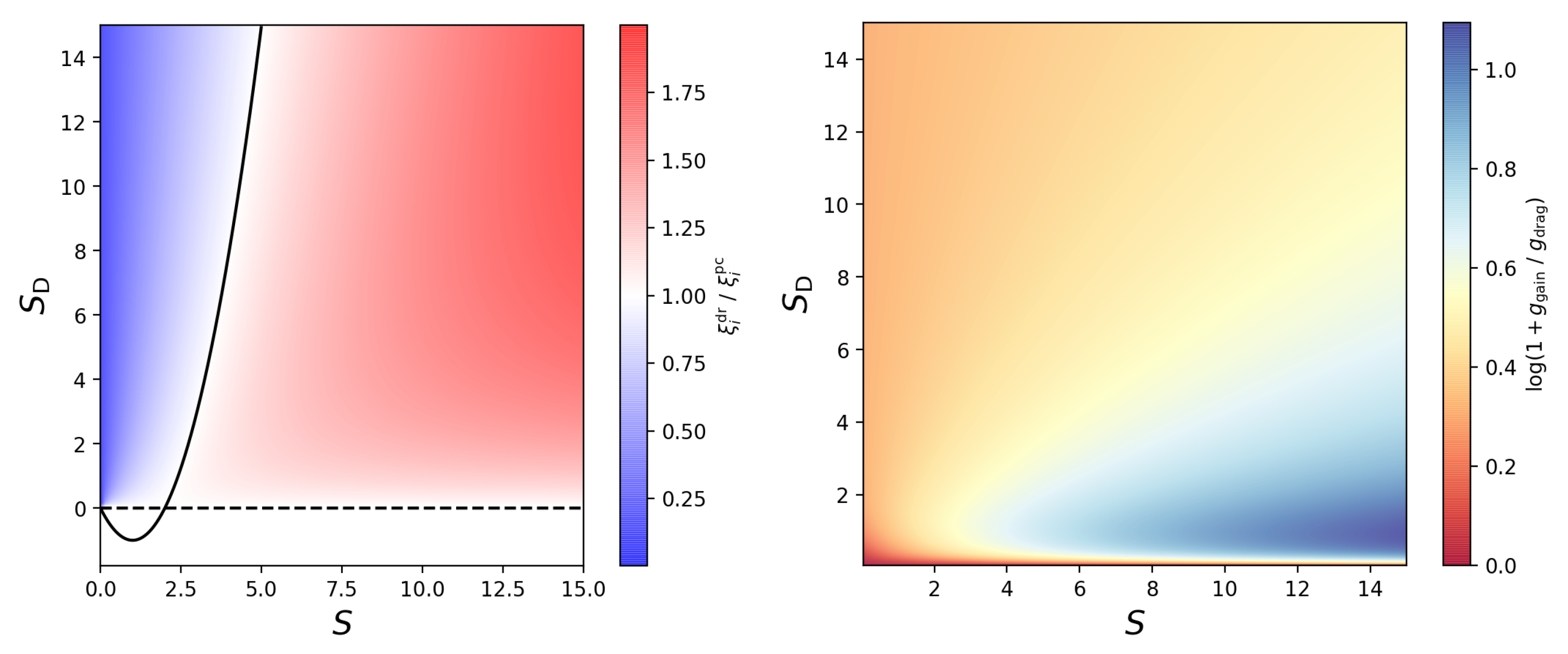
where the subscript “pc” refers to “position coupling”, i.e., no drift and we are assuming the gas-density profile and molecular abundances are the same in both cases. This indicates that slow winds tend to display slower grain growth in the presence of drift, while fast winds display an accelerated growth (see Figure 1 for a graphical representation of ${\xi }_{\mathrm{dr}}/{\xi }_{\mathrm{pc}}$). Furthermore, we note that there exist certain combinations of drift and wind velocities for which there is no difference in the grain-growth velocity ${\xi }_i$, whether there is drift or not, i.e., ${\xi }_{\mathrm{dr}}/{\xi }_{\mathrm{pc}}=1$. Setting ${\xi }_{\mathrm{dr}}/{\xi }_{\mathrm{pc}}=1$ in Equation (10) and solving for real $S_{\mathrm{D}}$ yields $S_{\mathrm{D},1}=S^2-2S$, which is shown as the solid black line in Figure 1. Consequently, we have ${\mathfrak{F}}_{\mathrm{D},1}+1=S$, suggesting that if the drift factor ${\mathfrak{F}}_{\mathrm{D}}$ increases proportional to S, the net effect on the grain-growth rate may be zero. Note that the part below $S_{\mathrm{D}}=0$ in Figure 1 is not relevant for a stationary mean-flow model, so ${\mathfrak{F}}_{\mathrm{D},1}<0$ will not occur.

3.3. Wind Acceleration, Drag and Growth: An Intricate Interplay between Forces

To first order, the dust opacity will simply scale with ${\mathfrak{F}}_{\mathrm{D}}$, so that ${\kappa }_{\mathrm{d}}\approx {\mathfrak{F}}_{\mathrm{D}}{\kappa }_{\mathrm{d}}^{\mathrm{pc}}$ and $F_{\mathrm{rad}}\approx {\mathfrak{F}}_{\mathrm{D}}{F}_{\mathrm{rad}}^{\mathrm{pc}}$. This scaling would be correct if the small-particle approximation is applicable and the number of dust grains is the same in both cases. In this limit, when $a\ll 2\pi \lambda$ ($\lambda$ is the wavelength of the incident radiation), absorption dominates over scattering, implying that ratio of the effective to the geometric cross-section is $Q=Q_{\mathrm{abs}}$, where $Q_{\mathrm{abs}}^{\prime }=Q_{\mathrm{abs}}/a_{\mathrm{gr}}$ becomes independent of the grain radius $a_{\mathrm{gr}}$. However, in detailed, explicitly time-dependent models, such as those by Sandin and Mattsson [23], there will be a distribution of different grain sizes at every r and also significant variance in the rate of grain nucleation, which is why this scaling cannot be entirely correct. However, as a general rule, the radiative acceleration of dust is greater if drift is included in the wind model.

In the CMC approximation, we have that the radiative acceleration approximately equals the acceleration owing to drag, i.e., $g_{\mathrm{rad}}=g_{\mathrm{drag}}=\sigma n_{\mathrm{d}}{v}_{\mathrm{D}}^2\vartheta \left(S_{\mathrm{D}}\right)$, where, assuming specular collisions only, the drag coefficient is given by [27]

$$\vartheta \left(S_{\mathrm{D}}\right)=\left[\frac{4S_{\mathrm{D}}^4+4S_{\mathrm{D}}^2-1}{4S_{\mathrm{D}}^4}\mathrm{erf}\left(S_{\mathrm{D}}\right)+\frac{2S_{\mathrm{D}}^2+1}{2\pi {\sqrt{S}}_{\mathrm{D}}^3}exp(-S_{\mathrm{D}}^2)\right].$$

(11)

However, this is not entirely correct if we study a region of the wind where the grains are growing rapidly by the accretion of molecules. There should be an extra term in the equation of motion that describes the dust condensation rate and the increase in grain mass [23]. Under most conditions, this term is negligible with regard to the overall wind acceleration and has little effect in general. However, in an outflow with a moderate amount of gas–dust drift, the deceleration effect can be 5–10 percent or more, depending on the conditions for grain growth. A graphical representation of this is shown in Figure 1 (right panel), where the deceleration owing to dust condensation $g_{\mathrm{gain}}$ is normalised to the mass fraction $X_i$ of the growth species i ($X_i\sim 0.01$) in the gas.

3.4. A New Correlation between Wind Properties and ${\mathfrak{F}}_{\mathrm{D}}$

Ideally, one would use detailed wind models with drift as input to stellar evolution calculations, but this is a matter of computational economy. It is known that the drift factor ${\mathfrak{F}}_{\mathrm{D}}$ correlates with the wind properties of simulated winds of carbon stars [23], which may provide a solution. However, it is not yet known if these correlations are the same for all parameter spaces (including Mira-type AGB stars), and we need to know the mass-loss rate $\dot{M}$ in any case. Below, we present a new correlation, which appears to be universal, at least for carbon stars, and may be used to estimate drift effects.

Elitzur and Ivezić [35] found that $\dot{M}\propto u_{\mathrm{out}}^3$ for optically thin winds, which is consistent with observations (see, e.g., the results of Schöier and Olofsson [36]). For optically thick winds, there is also a dependence on reddening, while luminosity dependence is weak owing to the drift effects. Based on the findings of Elitzur and Ivezić [35], we hypothesise that $\dot{M}{u}_{\mathrm{out}}^3=\varphi \left({\mathfrak{F}}_{\mathrm{D}}\right)$, where $\varphi$ is a simple function of ${\mathfrak{F}}_{\mathrm{D}}$, e.g., a power-law. In Figure 2, we show $\dot{M}{u}_{\mathrm{out}}^3$ as a function of ${\mathfrak{F}}_{\mathrm{D}}$ for the wind models with drift presented by Sandin and Mattsson [23]. As one can clearly see, there is a strong correlation. Fitting a straight line to the data (solid line in Figure 2, left panel) yields, $log\left(\dot{M}{u}_{\mathrm{out}}^3\right)=0.55-6.3log{\mathfrak{F}}_{\mathrm{D}}$. If we take this relation at face value, it can be used to estimate ${\mathfrak{F}}_{\mathrm{D}}$ for a given $\dot{M}$ in a stationary mean-flow wind model by the following algorithm:

• Assume ${\mathfrak{F}}_{\mathrm{D}}=1$ and compute the wind-velocity profile and grain growth from the equations given in Section 2 for a prescribed value of $\dot{M}$;
• Use the correlation above to infer the corresponding ${\mathfrak{F}}_{\mathrm{D}}$ and calculate the wind-velocity profile and grain growth again, now using the adjusted ${\mathfrak{F}}_{\mathrm{D}}$ value (which is assumed to be the same throughout the wind region);
• Repeat step 2 until the difference between the current ${\mathfrak{F}}_{\mathrm{D}}$ and the previous value is less than a predefined target value $\Delta {\mathfrak{F}}_{\mathrm{D}}^{\min }$.

4. Discussion

4.1. Why Should We Bother?

Drift is known to be a computational challenge in wind modelling [22] and it has been argued that effects of drift on wind formation are often relatively small [34]. Against that background, it seems we need to ensure that it is worthwhile to add drift to the model. Is it really worth the effort? To answer this question, we shall first consider the right panel in Figure 2. Clearly, there is a significant scatter in $\dot{M}$ values obtained with and without drift, indicating important differences in the net radiative forcing. Assuming no drift must be wrong to some extent, but it greatly simplifies the simulation of winds, which is likely the reason why the drift problem has received so little attention in recent years.

There are two fundamental reasons why “position coupling” can never be a viable approximation. First, the EOM cannot be derived from physics; what one does is replace the drag force $F_{\mathrm{drag}}$ with the radiative force $F_{\mathrm{rad}}$ owing to dust and assume that $v=u$ everywhere, at any time. Replacing $F_{\mathrm{drag}}$ with $F_{\mathrm{rad}}$ is justifiable provided that CMC can be assumed. However, $v=u$ implies there is no kinetic drag ($v_{\mathrm{D}}=0$), which makes this completely ad hoc and, in fact, inconsistent with the basic idea of a dust-driven wind, i.e., that the dust drags the gas along as it is accelerated by the radiation field.

The second reason, is that dust grains are an example of so-called “inertial particles” (essentially, finite-size particles with the property of mass), but, in this context they are predominantly accelerated by the force exerted upon them by the radiation field rather than kinetic drag from the carrier (gas). A dust grain has a finite mass, and thus it must have inertia. Any particle with the slightest amount of inertia will decouple from its carrier fluid, albeit by very little, as in the case of very small particles. If sufficiently small, they can effectively be regarded as massless, and if no other forces are acting upon them aside from the drag force from the carrier (and there is no back-reaction on the carrier), they may be treated as tracer particles or a coupled passive scalar fluid. In such a case, one can say that $v=u$ holds in the tracer-particle limit. However, when dust grains are radiatively accelerated and exert drag on the gas, the dust is no longer a passive scalar or tracer in the model—the grains become a dynamically active component which transfers momentum. Then, $v=u$ is not justifiable. In other words, denying the existence of inertia is completely unphysical, especially in the presence of external forces.

If we accept that drift is essential and, as seen in recent numerical work [23], can be very significant (with ${\mathfrak{F}}_{\mathrm{D}}\approx 5$ in some cases), it appears necessary to also include drift effects in the simplistic wind models used in stellar evolution codes.

4.2. Is Complete Momentum Coupling Applicable?

In deriving the simplified EOM of the wind (Equation (5)) we assumed that CMC would hold, at least on average. Sandin and Mattsson [23] have indeed showed that CMC appears to hold once an outflow has formed (see their appendix G). CMC can, in principle, hold generally, given that the advection of dust is locally balanced with acceleration so that a force equilibrium is maintained. For a stationary (or mean-flow) wind model, such an equilibrium is not obviously possible in the wind-acceleration zone. However, one could assume that the wave pressure $P_{\mathrm{w}/\mathrm{t}}$ affects both gas and dust is such a way that CMC holds on average. We therefore argue that CMC is a reasonable assumption that greatly simplifies the wind modelling in stellar evolution codes. The overall validity of the CMC needs to be verified by further detailed simulation, however.

4.3. Can One Estimate the Drift Velocity from the Simple Wind Model?

The short answer is yes, and this is useful in the algorithm presented above. As it makes use of the correlation in Figure 2, it may not always converge in just a few iterations if the actual ${\mathfrak{F}}_{\mathrm{D}}$ is high and $u_{\mathrm{out}}$ is small, in which case the method can become a computational bottleneck. However, there is a way to make a better initial guess than ${\mathfrak{F}}_{\mathrm{D}}=1$. If we recall Equation (9), we may note that $v_{\mathrm{D}}$ can be estimated from parameters that are all part of the wind model. That is, this simple estimate of $v_{\mathrm{D}}$ can be used to close the system of equations for the wind and dust growth. However, we emphasise that this system is only closed if the mass-loss $\dot{M}$ is known; we still need a prescription for $\dot{M}$, which is either based on models including drift or includes a correction for drift, as suggested in Section 3.4. However, since we know the wind velocity is typically $u\sim 10$ km s⁻¹ and $\langle Q_{\mathrm{ext}}\rangle \sim 1$, we can obtain a good indication of whether ${\mathfrak{F}}_{\mathrm{D}}$ is close to unity or not, which is important in order to minimise the number of iterations.

Do we really need to use the correlation in Figure 2 and the iterative scheme suggested in Section 3.4? It may seem that assuming CMC would be sufficient to find a system of equations that provides a basic correction for drift for a given $\dot{M}$. However, this is only a passable road forward if Equation (9) provides a sufficiently accurate estimate of $v_{\mathrm{D}}$. Unfortunately, we cannot assume it does, in general, because the resultant amount of drift when the terminal wind velocity is reached depends on several other factors as well—even if detailed models suggest it is a very good approximation in many cases (see, e.g., Figure 8 in Sandin and Mattsson [23]). Moreover, can we be certain that the mass-loss prescription used is sufficiently accurate? Sandin and Mattsson [23] showed that $\dot{M}$ is significantly different if drift is considered (note the scatter in Figure 2, right panel), which means that commonly used formulae, such as those by Blöcker [8] and Wachter et al. [9], are incorrect owing to the underlying zero-drift assumption as well as other factors [12].

4.4. A Grid of Mass-Loss Models as Input

Mattsson [37] suggested interpolation in a grid of detailed mass-loss models is the best way to prescribe mass-loss in models of AGB evolution. This conclusion relies on very extensive testing of various numerical approaches carried out by Mattsson [37], which demonstrated the need for a correct pre-interpolation in order to obtain sufficient accuracy and speed at the same time. The work by Mattsson [37] also includes the first ever results obtained from implementing this model-grid-interpolation approach in a stellar evolution code [38]. For that purpose, a simple Fortran code was created, which is now available via Zenodo [39]. The Mattsson [37] code has been used by Bladh et al. [15], Marigo et al. [40] and others, with updated input data for carbon stars. A modified version of the code has also been provided by Bladh et al. for use with a model grid for M-type (oxygen-rich) AGB stars [18].

None of the studies mentioned above include effects of drift and the grids are made with low spatial resolution models. The recent work by Sandin and Mattsson [23] has clearly demonstrated the need for both these improvements, but increased realism and precision comes at a price: the CPU time needed to produce a sufficiently long time series is well above hundred times longer. At present, only a handful of models have been produced and generating large grids does not seem feasible in the near future. That said, we would like to emphasise that a grid of mass-loss models as input to stellar evolution modelling is still likely the best way forward, despite the computational cost. Zero-drift (single-fluid) models of dust-driven winds from AGB stars are never going to be satisfactory as input, since typical drift velocities are of the same order as gas velocities of the outflows [23].

5. Conclusions

We have investigated the basis for including effects of gas-dust drift in the simplified wind models used in stellar evolution codes. We have shown that, while the EOM for the gas will be of the same form under the assumption of CMC, the dust-growth rate and wind acceleration can be very different compared to the no-drift case. Fast winds with significant drift tend to require significantly higher dust-growth rates, while very slow winds may have low dust-growth rates in case of drift. The latter may perhaps seem a little counter-intuitive, but is simply a consequence of how the dust-to-gas mass ratio changes when $v_{\mathrm{D}}\gg u$. In general, however, we expect drift to give more dust growth.

We have also demonstrated that there seems to be a tight anti-correlation between $\dot{M}{u}_{\mathrm{out}}^3$ and the drift factor ${\mathfrak{F}}_{\mathrm{D}}$. For a given mass-loss rate $\dot{M}$, one can thus find the corresponding ${\mathfrak{F}}_{\mathrm{D}}$ by iteration, i.e., solving the EOM repeatedly while updating ${\mathfrak{F}}_{\mathrm{D}}$ according to the correlation with $\dot{M}{u}_{\mathrm{out}}^3$ until convergence is obtained. However, since $\dot{M}$ is not known very well and existing mass-loss prescriptions are often based on wind models without drift, we argue that the input $\dot{M}$ must be anchored to detailed simulations of dust-driven winds with drift, such as those by Sandin and Mattsson [23]. This highlights the need to produce new grids of wind models to replace existing ones obtained under the assumption of no drift.

References

- Marini, E.; Dell’Agli, F.; Groenewegen, M.A.T.; García-Hernández, D.A.; Mattsson, L.; Kamath, D.; Ventura, P.; D’Antona, F.; Tailo, M. Understanding the evolution and dust formation of carbon stars in the LMC with a look at the JWST. arXiv 2020, arXiv:2012.12289. [Google Scholar]
- Marini, E.; Dell’Agli, F.; Di Criscienzo, M.; Puccetti, S.; García-Hernández, D.A.; Mattsson, L.; Ventura, P. Discovery of Stars Surrounded by Iron Dust in the Large Magellanic Cloud. Astrophys. J. Lett. 2019, 871, L16. [Google Scholar] [CrossRef]
- Dell’Agli, F.; García-Hernández, D.A.; Ventura, P.; Schneider, R.; Di Criscienzo, M.; Rossi, C. AGB stars in the SMC: Evolution and dust properties based on Spitzer observations. Mon. Not. R. Astron. Soc. 2015, 454, 4235–4249. [Google Scholar] [CrossRef] [Green Version]
- Matsuura, M.; Wood, P.R.; Sloan, G.C.; Zijlstra, A.A.; van Loon, J.T.; Groenewegen, M.A.T.; Blommaert, J.A.D.L.; Cioni, M.R.L.; Feast, M.W.; Habing, H.J.; et al. Spitzer observations of acetylene bands in carbon-rich asymptotic giant branch stars in the Large Magellanic Cloud. Mon. Not. R. Astron. Soc. 2006, 371, 415–420. [Google Scholar] [CrossRef] [Green Version]
- Ferrarotti, A.S.; Gail, H.P. Composition and quantities of dust produced by AGB-stars and returned to the interstellar medium. Astron. Astrophys. 2006, 447, 553–576. [Google Scholar] [CrossRef]
- Ventura, P.; di Criscienzo, M.; Schneider, R.; Carini, R.; Valiante, R.; D’Antona, F.; Gallerani, S.; Maiolino, R.; Tornambé, A. The transition from carbon dust to silicate production in low-metallicity asymptotic giant branch and super-asymptotic giant branch stars. Mon. Not. R. Astron. Soc. 2012, 420, 1442–1456. [Google Scholar] [CrossRef] [Green Version]
- Nanni, A.; Bressan, A.; Marigo, P.; Girardi, L. Evolution of thermally pulsing asymptotic giant branch stars-II. Dust production at varying metallicity. Mon. Not. R. Astron. Soc. 2013, 434, 2390–2417. [Google Scholar] [CrossRef] [Green Version]
- Blöcker, T. Stellar evolution of low and intermediate-mass stars. I. Mass loss on the AGB and its consequences for stellar evolution. Astron. Astrophys. 1995, 297, 727–738. [Google Scholar]
- Wachter, A.; Schröder, K.P.; Winters, J.M.; Arndt, T.U.; Sedlmayr, E. An improved mass-loss description for dust-driven superwinds and tip-AGB evolution models. Astron. Astrophys. 2002, 384, 452–459. [Google Scholar] [CrossRef] [Green Version]
- Guandalini, R.; Busso, M.; Ciprini, S.; Silvestro, G.; Persi, P. Infrared photometry and evolution of mass-losing AGB stars. I. Carbon stars revisited. Astron. Astrophys. 2006, 445, 1069–1080. [Google Scholar] [CrossRef] [Green Version]
- Mattsson, L.; Wahlin, R.; Höfner, S.; Eriksson, K. Intense mass loss from C-rich AGB stars at low metallicity? Astron. Astrophys. 2008, 484, L5–L8. [Google Scholar] [CrossRef] [Green Version]
- Mattsson, L.; Wahlin, R.; Höfner, S. Dust driven mass loss from carbon stars as a function of stellar parameters. I. A grid of solar-metallicity wind models. Astron. Astrophys. 2010, 509, A14. [Google Scholar] [CrossRef]
- Mattsson, L.; Höfner, S. Dust-driven mass loss from carbon stars as a function of stellar parameters. II. Effects of grain size on wind properties. Astron. Astrophys. 2011, 533, A42. [Google Scholar] [CrossRef]
- Mattsson, L.; Aringer, B.; Andersen, A.C. How Important Are Metal-Poor AGB Stars As Cosmic Dust Producers? In Why Galaxies Care about AGB Stars III: A Closer Look in Space and Time; Astronomical Society of the Pacific Conference Series; Kerschbaum, F., Wing, R.F., Hron, J., Eds.; ASP: San Francisco, CA, USA, 2015; Volume 497, pp. 385–390. [Google Scholar]
- Bladh, S.; Eriksson, K.; Marigo, P.; Liljegren, S.; Aringer, B. Carbon star wind models at solar and sub-solar metallicities: A comparative study. I. Mass loss and the properties of dust-driven winds. Astron. Astrophys. 2019, 623, A119. [Google Scholar] [CrossRef] [Green Version]
- Höfner, S. Winds of M-type AGB stars driven by micron-sized grains. Astron. Astrophys. 2008, 491, L1–L4. [Google Scholar] [CrossRef] [Green Version]
- Höfner, S.; Bladh, S.; Aringer, B.; Ahuja, R. Dynamic atmospheres and winds of cool luminous giants. I. Al2O3 and silicate dust in the close vicinity of M-type AGB stars. Astron. Astrophys. 2016, 594, A108. [Google Scholar] [CrossRef] [Green Version]
- Bladh, S.; Liljegren, S.; Höfner, S.; Aringer, B.; Marigo, P. An extensive grid of DARWIN models for M-type AGB stars. I. Mass-loss rates and other properties of dust-driven winds. Astron. Astrophys. 2019, 626, A100. [Google Scholar] [CrossRef] [Green Version]
- Sandin, C.; Höfner, S. Three-component modeling of C-rich AGB star winds. I. Method and first results. Astron. Astrophys. 2003, 398, 253–266. [Google Scholar] [CrossRef] [Green Version]
- Sandin, C.; Höfner, S. Three-component modeling of C-rich AGB star winds. II. The effects of drift in long period variables. Astron. Astrophys. 2003, 404, 789–807. [Google Scholar] [CrossRef]
- Sandin, C.; Höfner, S. Three-component modeling of C-rich AGB star winds. III. Micro-physics of drift-dependent dust formation. Astron. Astrophys. 2004, 413, 789–798. [Google Scholar] [CrossRef] [Green Version]
- Sandin, C. Three-component modelling of C-rich AGB star winds. IV. Revised interpretation with improved numerical descriptions. Mon. Not. R. Astron. Soc. 2008, 385, 215–230. [Google Scholar] [CrossRef] [Green Version]
- Sandin, C.; Mattsson, L. Three-component modelling of C-rich AGB star winds - V. Effects of frequency-dependent radiative transfer including drift. Mon. Not. R. Astron. Soc. 2020, 499, 1531–1560. [Google Scholar] [CrossRef]
- Mattsson, L. Winds of AGB stars:. the two roles of atmospheric dust. Mem. Soc. Astron. Ital. 2016, 87, 249. [Google Scholar]
- Krüger, D.; Gauger, A.; Sedlmayr, E. Two-fluid models for stationary dust-driven winds. I. Momentum and energy balance. Astron. Astrophys. 1994, 290, 573–589. [Google Scholar]
- Krüger, D.; Patzer, A.B.C.; Sedlmayr, E. On the growth of carbonaceous grains in circumstellar envelopes. Astron. Astrophys. 1996, 313, 891–896. [Google Scholar]
- Schaaf, S.A. Mechanics of Rarefied Gases. In Handbuch der Physik: Strömungsmechanik II; Springer: Berlin, Germany, 1963; Volume VIII/2, pp. 591–624. [Google Scholar]
- Gail, H.P.; Sedlmayr, E. Mineral formation in stellar winds. I. Condensation sequence of silicate and iron grains in stationary oxygen rich outflows. Astron. Astrophys. 1999, 347, 594–616. [Google Scholar]
- Lucy, L.B. The Formation of Resonance Lines in Extended and Expanding Atmospheres. Astrophys. J. 1971, 163, 95. [Google Scholar] [CrossRef]
- Lucy, L.B. Mass Loss by Cool Carbon Stars. Astrophys. J. 1976, 205, 482–491. [Google Scholar] [CrossRef]
- Gilman, R.C. On the Coupling of Grains to the Gas in Circumstellar Envelopes. Astrophys. J. 1972, 178, 423–426. [Google Scholar] [CrossRef]
- Kwok, S. Radiation pressure on grains as a mechanism for mass loss in red giants. Astrophys. J. 1975, 198, 583–591. [Google Scholar] [CrossRef]
- Habing, H.J.; Tignon, J.; Tielens, A.G.G.M. Calculations of the outflow velocity of envelopes of cool giants. Astron. Astrophys. 1994, 286, 523–534. [Google Scholar]
- Höfner, S.; Olofsson, H. Mass loss of stars on the asymptotic giant branch. Mechanisms, models and measurements. Astron. Astrophys. 2018, 26, 1. [Google Scholar] [CrossRef] [Green Version]
- Elitzur, M.; Ivezić, Ž. Dusty winds - I. Self-similar solutions. Mon. Not. R. Astron. Soc. 2001, 327, 403–421. [Google Scholar] [CrossRef] [Green Version]
- Schöier, F.L.; Olofsson, H. Models of circumstellar molecular radio line emission. Mass loss rates for a sample of bright carbon stars. Astron. Astrophys. 2001, 368, 969–993. [Google Scholar] [CrossRef] [Green Version]
- Mattsson, L. On the Winds of Carbon Stars and the Origin of Carbon: A Theoretical Study; Acta Universitatis Upsaliensis: Uppsala, Sweden, 2009. [Google Scholar]
- Paxton, B.; Bildsten, L.; Dotter, A.; Herwig, F.; Lesaffre, P.; Timmes, F. Modules for Experiments in Stellar Astrophysics (MESA). Astrophys. J. Suppl. Ser. 2011, 192, 3. [Google Scholar] [CrossRef]
- Mattsson, L. Dust driven mass loss from carbon stars as a function of stellar parameters.-A Fortran module for use in stellar evolution codes. 2021; unpublished. [Google Scholar]
- Marigo, P.; Cummings, J.D.; Curtis, J.L.; Kalirai, J.; Chen, Y.; Tremblay, P.E.; Ramirez-Ruiz, E.; Bergeron, P.; Bladh, S.; Bressan, A.; et al. Carbon star formation as seen through the non-monotonic initial-final mass relation. Nat. Astron. 2020, 4, 1102–1110. [Google Scholar] [CrossRef]
Figure 1.
Left: Growth velocity for efficient grain growth in a wind with drift relative to that of a scenario without drift, as a function of drift velocity relative to the thermal speed of the gas () and outflow velocity relative to the same (S). The solid black line marks the combinations of and S, for which there is no net effect of drift. The trivial case () is marked by the dashed line. The (white) region below this line corresponds to negative drift and is not considered, since negative drift is impossible for a stationary mean-flow component. Right: Comparison of the deceleration owing to grain growth () to the acceleration via drag (). Note that has been normalised to the mass fraction of the growth species in the gas – the physical ratio is much smaller.
Figure 2.
Left: Correlation between and the drift factor , confirming the proposed relationship in Section 3.4. It is likely, but still not confirmed, that a similar correlation exists for wind models of Mira-type stars. Right: Scatter plot of mass-loss rates obtained with drift (ordinate axis labelled “dr”) and without (abscissa axis labelled “pc”).
Publisher’s Note: MDPI stays neutral with regard to jurisdictional claims in published maps and institutional affiliations. |
© 2021 by the authors. Licensee MDPI, Basel, Switzerland. This article is an open access article distributed under the terms and conditions of the Creative Commons Attribution (CC BY) license (https://creativecommons.org/licenses/by/4.0/).
Share and Cite
MDPI and ACS Style
Mattsson, L.; Sandin, C. AGB Winds with Gas-Dust Drift in Stellar Evolution Codes. Universe 2021, 7, 113. https://doi.org/10.3390/universe7050113
AMA Style
Mattsson L, Sandin C. AGB Winds with Gas-Dust Drift in Stellar Evolution Codes. Universe. 2021; 7(5):113. https://doi.org/10.3390/universe7050113
Chicago/Turabian StyleMattsson, Lars, and Christer Sandin. 2021. "AGB Winds with Gas-Dust Drift in Stellar Evolution Codes" Universe 7, no. 5: 113. https://doi.org/10.3390/universe7050113
Note that from the first issue of 2016, this journal uses article numbers instead of page numbers. See further details here.