
Abstract
Depopulation of birds has been authenticated to be an effective measure in controlling avian influenza transmission. In this work, we establish a Filippov avian-only model incorporating a threshold policy control. We choose the index—the maximum between the infected threshold level \(I_{T}\) and the product of the number of susceptible birds S and a ratio threshold value ξ—to decide on whether to trigger the control measures or not, which then leads to a discontinuous separation line and two pieces of sliding-mode domains. Meanwhile, one more sliding-mode domain gives birth to more complex dynamics. We investigate the global dynamical behavior of the Filippov model, including the real and/or virtual equilibria and the two sliding modes and their dynamics. The solutions will eventually stabilize at the real endemic equilibrium of the subsystem or the pseudoequilibria on the two sliding modes due to different threshold values. Therefore an effective and efficient threshold policy is essential to control the influenza by driving the number of infected birds below a certain level or at a previously given level.
1 Introduction
Highly pathogenic avian influenza A virus causes high flock mortality [1]. The disease not only causes significant social and economic loss on domestic fowl in affected areas [2] but composes a potentially serious threat for humans [3, 4]. Governments worldwide have paid a lot to treat the patients and control the pandemic [5]. Hence, it is an emergent issue to identify any effective control strategies to eliminate the influenza or at least to reduce the impact to a tolerant level; in particular, bringing down the number of infected birds becomes a priority.
The Chinese government has begun to release avian influenza A(H7N9) data via websites and official news agency daily since the first case was reported in March 2013 [6]. Hence people could understand the progress and then avoid some unnecessary contact. At the same time, some cities like Nanjing, Guangzhou, and Shanghai have closed several poultry markets, culled poultry and disinfected the environment, and the first two measures were proved to be more effective in controlling A(H7N9) infections [7].
Indeed, depopulation of infected birds and those with close contact has been authenticated to be an effective measure in controlling avian influenza transmission, however, this is also a risky enterprise with the risk of killing the susceptible birds during the infection prevention [8, 9]. Therefore the identified culling strategy should not only be effective but also efficient to avoid overkilling of the susceptible birds, and then further establish a balance among acceptable control measures safeguarding the livelihoods of farmers and the health of the population [10].
Mathematical modeling is a useful tool and has been applied widely to illustrate the transmission dynamics of various pandemic diseases. Based on the epidemiology and different control strategies, ordinary differential equations [11, 12], delay differential equations [13–16], and discrete differential equations [17] have been proposed and analyzed. Andronicoa et al. [18] established a mathematical model to study the spatiotemporal evolution of the disease and evaluate the impact of control measures. The authors obtained that a faster culling of diagnosed infected targets would have a larger impact on the total number of infections.
Several conventional control methods considering a threshold policy may be employed in disease management. A threshold policy is such that there exists a tolerance threshold so that whenever the number of the infected is below that threshold, the infection is considered to be tolerable. Otherwise, the infection might cause intolerable economic damage. Mathematical models with a threshold policy, which is biologically and economically desirable, are described by the so-called Filippov systems with discontinuous right-hand sides [19–21].
Xiao et al. [22] extended the classical SIR model to a Filippov SIR model by including a piecewise incidence rate to represent behavioral change of general individuals and implementation of necessary precautionary measures. They suggested that choosing a proper combination of threshold and control intensities based on a threshold policy can preclude outbreaks or stabilize the infection at a desired level. Zhou et al. [23] proposed a Filippov-type model of interrupting transmission of West Nile virus to birds by implementing culling of mosquitoes once the number of infected birds exceeds a threshold level. They showed that strengthening the culling of mosquitoes together with protecting birds is a good choice in controlling the spread of West Nile virus. Bolzoni et al. [24] studied a two-patches metapopulation mathematical model in wildlife diseases. They considered both proactive end reactive localized culling strategies. The localized reactive control is described by a Filippov system with a piecewise-constant culling effort function. The authors indicated that when the host fecundity is affected by the infection, localized culling may be ineffective in controlling wildlife diseases.
Chong et al. [25] considered an avian-only model considering a threshold policy. The authors chose the number of infected birds as an index, that is, once the index exceeds the threshold level \(I_{T}\), culling of infected birds is employed, otherwise, no action is taken. However, when the number of infected birds exceeds the threshold level \(I_{T}\) and the number of susceptible birds is large enough, it is not always necessary to take control strategies. In fact, if the interaction ratio of the number of infected and susceptible birds is smaller than a ratio threshold value, then more effort is needed to take care of the susceptible birds to maximize the profits rather than to take control strategies, which then could lead to labor shortage and cause economic loss for farmers. This nonsmooth threshold mechanism has been adopted by Li et al. [26] for a plant disease model. Therefore, reconsidering the avian-only model in [25] by incorporating this kind of a threshold policy may be more reasonable, which also results in a nonsmooth separation line compared to the model in [25].
The rest of the paper is structured as follows. In Sect. 2, we establish an avian-only Filippov model with considering a more realistic threshold policy which leads to a nonsmooth separation line. The dynamical behavior of the proposed Filippov system, including the real and/or virtual equilibria, the two sliding-mode domains and their dynamics is investigated in Sects. 3–5. We conclude this work in Sect. 6.
2 Filippov avian-only model
In order to better control the avian influenza transmission, minimize the economic damage, and optimize the profits, control strategies should be applied based on whether the number of infected birds and/or the interaction ratio of the number of infected and susceptible birds exceed the given tolerant threshold levels or not. If the number of infected birds is below the infected threshold level \(I_{T}\), then no control is taken; above \(I_{T}\), the control strategies should be carried out depending on the number of susceptible birds and the interaction ratio of the number of infected and susceptible birds. When the number of susceptible birds S is small (\(S<\frac{I_{T}}{\xi }\)), we cull infected birds at a rate of \(c_{2}\) and susceptible birds at a rate of \(c_{1}\), \(c_{i}>0, i=1,2\), respectively. Whilst when the number of susceptible birds is large enough (\(S>\frac{I_{T}}{\xi }\)) and the interaction ratio is below the ratio threshold value ξ, which means the number of infected birds is relatively small compared to the susceptible birds, then the control strategy is not taken to save the effort and maximize the profits; otherwise, if the interaction ratio exceeds the ratio threshold value ξ, control measures are triggered. A schematic diagram depicting the threshold policy is shown in Fig. 1. The reason for culling susceptible birds is that as the influenza progresses, more susceptible birds may be infected later and cause a more severe outbreak, here we assume \(c_{1}< c_{2}\).

Schematic diagram of the threshold policy
Chong et al. [25] assumed that the avian populations are subject to the rule of constant growth. But migrant birds are mostly viewed as the original infection source [12, 27]. Pathogens may be transmitted to new areas by migratory hosts, which leads to new host species’ exposure and potential infection. Then those resident hosts, which are immunologically naive to these novel pathogens, may subsequently act as local amplifiers [18]. For example, West Nile virus’s global spread is greatly facilitated by migratory birds, which transmit the pathogens to other wildlife and humans in many parts of the world [28]. It is well known that the logistic growth is more reasonable than the constant growth for the wildlife birds, including resident and migratory birds [12]. Hence, we choose logistic growth here for avian populations. Let \(S(t)\) and \(I(t)\) denote the numbers of susceptible and infected birds at time t. The susceptible birds are subject to logistic growth \(rS(1-S/K)\), where r is the intrinsic growth rate and K is the maximal carrying capacity.
Then the Filippov avian-only model with a nonsmooth separation line can be listed by the following system:
with
where β is the transmission rate of the disease from infected birds I to susceptible birds S, μ is the natural death rate, d is the disease-induced death rate. Here we assume \(r>c_{1}\) and \(\xi >0\); when \(\xi =0\), it becomes the model in [25] with constant growth.
Denote the nonsmooth separation line as \(\Omega =\{(S,I)\in R_{+}^{2}: H(S,I)=I-\max \{I_{T},\xi S\}=0\}\), then the \(S, I\) space \(R^{2}_{+}\) consists of the following four regions:
The dynamics in subregion \(G_{i}\) are governed by \(F_{i}\), \(i=1,2\), where
Note that the manifolds \(\Omega _{1}\) and \(\Omega _{2}\) are discontinuity surfaces connecting the two different structures of system (1)–(2). We consider the solutions of system (1)–(2) in Filippov’s sense, as the right-hand side of the system is discontinuous. The theory of existence and uniqueness of solutions of Filippov systems is developed and can be found in [29]. We present the definitions of real equilibrium, virtual equilibrium, sliding mode, and pseudoequilibrium that are necessary throughout the paper [26, 30–33].
Definition 2.1
\(E^{R}\) is called a real equilibrium of system (1)–(2) if \(F_{1}(E^{R})=0, E^{R}\in G_{1}\) or \(F_{2}(E^{R})=0, E^{R}\in G_{2}\); \(E^{V}\) is called a virtual equilibrium of system (1)–(2) if \(F_{1}(E^{V})=0, E^{V}\in G_{2}\) or \(F_{2}(E^{V})=0, E^{V}\in G_{1}\).
Definition 2.2
If there exists a subset Σ of the manifold \(\Omega _{i}\) such that the flows of f (outside of \(\Omega _{i}\)) are directed towards each other on them, \(i=1,2\), then Σ is called a sliding mode.
By applying the well-known Filippov convexity method [29] or Utkin’s equivalent control method [34], we can obtain the dynamics on the sliding mode. Here we present the Filippov convexity method, that is,
where \(\sigma = \frac{\langle \nabla H, F_{2}\rangle }{\langle \nabla H, F_{2}-F_{1}\rangle }\), \((\cdot )^{T}\) means the transpose of the vector, \(\langle \cdot, \cdot \rangle \) denotes the standard scalar product.
Definition 2.3
\(E^{P}\) is called a pseudoequilibrium if \(E^{P}\) is an equilibrium on the sliding mode Σ, that is, \(\Psi (E^{P})=0\) and \(E^{P}\in \Sigma \subset \Omega _{i}\), \(i=1,2\).
2.1 Dynamics in subregion \(G_{i}\), \(i=1,2\)
By applying the next generation matrix method [35], we can obtain the basic reproduction number \(R_{0i}\) for the system in region \(G_{i}\), \(i=1,2\),
The equilibria of the system in region \(G_{i}\) are two disease-free equilibria, \(E^{1}_{i0}\) and \(E^{2}_{i0}\), and a unique endemic equilibrium \(E_{i}=(S_{i}^{*}, I_{i}^{*})\) if \(R_{0i}>1\), \(i=1,2\), where
The system in subregions \(G_{1}\) and \(G_{2}\) has been studied with different methods, here we just present the main results; more detailed proofs can be found in [9, 12].
Proposition 2.1
(i) The disease-free equilibrium \(E^{1}_{i0}\) of the system in subregion \(G_{i}\) is always unstable; (ii) If \(R_{0i}\leq 1\), the disease-free equilibrium \(E^{2}_{i0}\) of the system in subregion \(G_{i}\) is globally asymptotically stable; (iii) If \(R_{0i}>1\), the endemic equilibrium \(E_{i}\) of the system in subregion \(G_{i}\) is globally asymptotically stable, \(i=1,2\).
In the following three sections (Sects. 3–5), we investigate the existence and global stability of the real equilibrium, virtual equilibrium, and the pseudoequilibria on the two sliding modes with different threshold values. By Proposition 2.1, we only consider the case when \(R_{0i}>1\), then system \(F_{i}\) in each subregion \(G_{i}\) admits the unique global asymptotical stable endemic equilibrium \(E_{i}\), \(i=1,2\). Since \(S_{1}^{*}< S_{2}^{*}\), we then consider the following three cases generated by \(S_{1}^{*}< S_{2}^{*}<\frac{I_{T}}{\xi }\), \(S_{1}^{*}<\frac{I_{T}}{\xi }<S_{2}^{*}\), and \(\frac{I_{T}}{\xi }< S_{1}^{*}< S_{2}^{*}\). We illustrate the dynamical behaviors of system (1)–(2) from one case to another.
3 Case A: global dynamics when \(S_{1}^{*}< S_{2}^{*}<\frac{I_{T}}{\xi }\) (\(\xi <\frac{I_{T}}{S_{2}^{*}}\))
3.1 Sliding mode on \(\Omega _{1}\) and its dynamics
Firstly, we present the existence of the sliding mode and its dynamics on the discontinuity surface \(\Omega _{1}\). Since the scalar function \(H(S,I)=I-I_{T}\) on \(\Omega _{1}\), \(\nabla H=(0,1)^{T}\), then it can be easily obtained that
For \(S_{1}^{*}< S_{2}^{*}<\frac{I_{T}}{\xi }\), therefore, by Definition 2.2 of the sliding mode, we can obtain the sliding-mode domain \(\Sigma _{1}\subset \Omega _{1}\) as follows:
Here, we apply the Filippov convexity method [36, 37] to obtain the sliding-mode dynamics along the sliding mode \(\Sigma _{1}\),
That is,
System (6) has a unique positive equilibrium, denoted by \(E_{p1}=(S_{p1}^{*}, I_{T})\), where
if \(I_{T}<\frac{r+\frac{c_{1}}{c_{2}}(\mu +d)}{\beta }=g_{1}\).
Next, we present the conditions for \(E_{p1}\) to be a pseudoequilibrium on \(\Sigma _{1}\subset \Omega _{1}\) and investigate its stability.
Proposition 3.1
\(E_{p1}\) is a pseudoequilibrium on \(\Sigma _{1}\subset \Omega _{1}\) if and only if \(S_{1}^{*}< S_{p1}^{*}< S_{2}^{*}\), that is, \(I_{2}^{*}< I_{T}< I_{1}^{*}\).
Theorem 3.1
\(E_{p1}\) is stable on \(\Sigma _{1}\subset \Omega _{1}\) when it is a pseudoequilibrium.
Proof
It can be obtained by simple calculation that
Hence, \(E_{p1}\) is stable. □
3.2 Sliding mode on \(\Omega _{2}\) and its dynamics
Since the scalar function \(H(S,I)=I-\xi S\) on \(\Omega _{2}\), \(\nabla H=(-\xi,1)^{T}\), then we can obtain that
where
Denote
Obviously, we have \(H_{2}>H_{3}\), \(g_{1}< g_{2}< g_{3}\).
Proposition 3.2
According to different values of \(I_{T}\) and ξ, we have the following results:
-
(i)
If \(I_{T}< g_{2}\) and \(\xi >H_{2}\), then \(\frac{I_{T}}{\xi }< S^{-}\) and the sliding-mode domain on \(\Omega _{2}\) is
$$ \Sigma _{2}= \bigl\{ (S,I)\in \Omega _{2}: S^{-}< S< S^{+} \bigr\} ; $$ -
(ii)
If \(I_{T}< g_{2}\) and \(H_{3}<\xi <H_{2}\) or \(g_{2}< I_{T}< g_{3}\) and \(\xi >H_{3}\), then \(S^{-}<\frac{I_{T}}{\xi }<S^{+}\) and the sliding-mode domain on \(\Omega _{2}\) is
$$ \Sigma _{2}= \biggl\{ (S,I)\in \Omega _{2}: \frac{I_{T}}{\xi }< S< S^{+} \biggr\} ; $$ -
(iii)
If \(I_{T}>g_{3}\) or \(I_{T}< g_{3}\) and \(\xi < H_{3}\), then \(S^{+}<\frac{I_{T}}{\xi }\) and there does not exist a sliding-mode domain on \(\Omega _{2}\).
Agian, we apply the Filippov convexity method [36, 37] to obtain the sliding-mode dynamics along the sliding mode \(\Sigma _{2}\),
That is,
System (7) admits a unique positive equilibrium \(E_{p2}=(S_{p2}^{*}, \xi S_{p2}^{*})\), where
Theorem 3.2
\(E_{p2}\) is stable on \(\Sigma _{2}\subset \Omega _{2}\) when it is a pseudoequilibrium.
Proof
We have
since \(c_{1}< c_{2}\). Hence, \(E_{p2}\) is stable. □
The following result gives the conditions for \(E_{p2}\) to be a pseudoequilibrium on \(\Sigma _{2}\subset \Omega _{2}\).
Proposition 3.3
According to the relationship between \(S^{-}, S^{+}\), and \(\frac{I_{T}}{\xi }\), we have:
-
(i)
If \(\frac{I_{T}}{\xi }< S^{-}\), that is, \(I_{T}< g_{2}\) and \(\xi >H_{2}\), \(E_{p2}\) becomes a pseudoequilibrium on \(\Sigma _{2}\subset \Omega _{2}\) if and only if
$$ \frac{I_{2}^{*}}{S_{2}^{*}}< \xi < \frac{I_{1}^{*}}{S_{1}^{*}}; $$ -
(ii)
If \(S^{-}<\frac{I_{T}}{\xi }<S^{+}\), that is, \(I_{T}< g_{2}\) and \(H_{3}<\xi <H_{2}\) or \(g_{2}< I_{T}< g_{3}\) and \(\xi >H_{3}\), \(E_{p2}\) becomes a pseudoequilibrium on \(\Sigma _{2}\subset \Omega _{2}\) if and only if
$$ I_{T}< g_{1} \quad\textit{and}\quad \xi >\max \biggl\{ \frac{I_{2}^{*}}{S_{2}^{*}}, H_{1} \biggr\} . $$
Proof
(i) If \(\frac{I_{T}}{\xi }< S^{-}\), then \(E_{p2}\) becomes a pseudoequilibrium on \(\Sigma _{2}\subset \Omega _{2}\) if and only if \(S^{-}< S_{p2}^{*}< S^{+}\). On the other hand, we have
Similarly, \(S_{p2}^{*}< S^{+}\Longleftrightarrow \xi >\frac{I_{2}^{*}}{S_{2}^{*}}\). Hence, the result is obtained.
(ii) If \(S^{-}<\frac{I_{T}}{\xi }<S^{+}\), then \(E_{p2}\) becomes a pseudoequilibrium on \(\Sigma _{2}\subset \Omega _{2}\) if and only if \(\frac{I_{T}}{\xi }< S_{p2}^{*}< S^{+}\). And
Together with \(S_{p2}^{*}< S^{+}\), that is, \(\xi >\frac{I_{2}^{*}}{S_{2}^{*}}\), one can obtain the result. □
The next proposition will play a crucial role in the following analysis.
Proposition 3.4
We have:
-
\(I_{T}< I_{2}^{*}\) if and only if \(H_{1}< H_{3}<H_{2}, H_{1}<\frac{I_{2}^{*}}{S_{2}^{*}}, H_{3}< \frac{I_{2}^{*}}{S_{2}^{*}}, \frac{I_{T}}{S_{2}^{*}}>H_{1}, \frac{I_{T}}{S_{2}^{*}}>H_{3}, \frac{I_{T}}{S_{2}^{*}}< \frac{I_{2}^{*}}{S_{2}^{*}}\);
-
\(I_{2}^{*}< I_{T}< I_{1}^{*}\) if and only if \(H_{3}< H_{1}<H_{2}\);
-
\(I_{T}>I_{1}^{*}\) if and only if \(H_{3}< H_{2}<H_{1}, H_{1}>\frac{I_{1}^{*}}{S_{1}^{*}}, H_{2}> \frac{I_{1}^{*}}{S_{1}^{*}}, \frac{I_{T}}{S_{1}^{*}}<H_{1}, \frac{I_{T}}{S_{1}^{*}}<H_{2}, \frac{I_{T}}{S_{1}^{*}}> \frac{I_{1}^{*}}{S_{1}^{*}}\).
Proof
Here we present the proof for \(I_{T}< I_{2}^{*}\Leftrightarrow H_{1}<\frac{I_{2}^{*}}{S_{2}^{*}}\), the other results can be obtained by applying the same method. There holds
Hence, the result is obtained. □
We present the relationships between the seven variables \(\frac{I_{i}^{*}}{S_{i}^{*}}, \frac{I_{T}}{S_{i}^{*}}, H_{j}, i=1,2, j=1,2,3\) related to \(I_{1}^{*}, I_{2}^{*}\), and \(I_{T}\), which play a vital role throughout the following analysis.
Proposition 3.5
We have:
-
(i)
If \(I_{T}< I_{2}^{*}< I_{1}^{*}\), then
$$ H_{1}< H_{3}< H_{2}< \frac{I_{T}}{S_{1}^{*}}< \frac{I_{1}^{*}}{S_{1}^{*}},\qquad H_{3}< \frac{I_{T}}{S_{2}^{*}}< \frac{I_{T}}{S_{1}^{*}},\qquad \frac{I_{T}}{S_{2}^{*}}< \frac{I_{2}^{*}}{S_{2}^{*}}< \frac{I_{1}^{*}}{S_{1}^{*}}; $$ -
(ii)
If \(I_{2}^{*}< I_{T}< I_{1}^{*}\), then
$$ \frac{I_{2}^{*}}{S_{2}^{*}}< \frac{I_{T}}{S_{2}^{*}}< H_{3}< H_{1}< H_{2}< \frac{I_{T}}{S_{1}^{*}}< \frac{I_{1}^{*}}{S_{1}^{*}}; $$ -
(ii)
If \(I_{2}^{*}< I_{1}^{*}< I_{T}\), then
$$ \frac{I_{2}^{*}}{S_{2}^{*}}< \frac{I_{T}}{S_{2}^{*}}< H_{3}< H_{2}< H_{1},\qquad \frac{I_{T}}{S_{2}^{*}}< \frac{I_{T}}{S_{1}^{*}}< H_{2},\qquad \frac{I_{2}^{*}}{S_{2}^{*}}< \frac{I_{1}^{*}}{S_{1}^{*}}< \frac{I_{T}}{S_{1}^{*}}. $$
Proof
We just prove the case if \(I_{2}^{*}< I_{T}< I_{1}^{*}\). When \(I_{T}< I_{2}^{*}< I_{1}^{*}\) or \(I_{2}^{*}< I_{1}^{*}< I_{T}\), the results can be obtained similarly by applying Proposition 3.4. By Proposition 3.4, there holds
Hence, the result is obtained following the above inequalities. □
3.3 Global dynamics
3.3.1 Case A.1: \(I_{T}< I_{2}^{*}< I_{1}^{*}\)
In this situation, \(E_{1}^{V}\) is a virtual equilibrium, whereas \(E_{2}^{R}\) is a real equilibrium. In this and the following analysis, we denote a possible real equilibrium by \(E_{i}^{R}\) and a possible virtual equilibrium by \(E_{i}^{V}\), \(i=1,2\), respectively. Furthermore, \(E_{p1}\) is never a pseudoequilibrium on \(\Sigma _{1}\subset \Omega _{1}\) by Proposition 3.1. For \(\frac{I_{T}}{S_{2}^{*}}<\frac{I_{2}^{*}}{S_{2}^{*}}< \frac{I_{1}^{*}}{S_{1}^{*}}\), \(E_{p2}\) is never a pseudoequilibrium on \(\Sigma _{2}\subset \Omega _{2}\) by Proposition 3.3. We can obtain the globally asymptotical stability of \(E_{2}^{R}\).
Theorem 3.3
\(E_{2}^{R}\) is globally asymptotically stable if \(S_{1}^{*}< S_{2}^{*}<\frac{I_{T}}{\xi }\) and \(I_{T}< I_{2}^{*}< I_{1}^{*}\).
-
If \(H_{1}< H_{3}<\frac{I_{T}}{S_{2}^{*}}<H_{2}<\frac{I_{T}}{S_{1}^{*}}< \frac{I_{1}^{*}}{S_{1}^{*}}\), then there does not exist a sliding-mode domain on \(\Omega _{2}\) when \(\xi < H_{3}\); the sliding-mode domain on \(\Omega _{2}\) is \(\Sigma _{2}=\{(S,I)\in \Omega _{2}: \frac{I_{T}}{\xi }< S< S^{+}\}\) when \(\xi >H_{3}\); as can be seen in Fig. 3(a);
-
If \(H_{1}< H_{3}< H_{2}<\frac{I_{T}}{S_{2}^{*}}<\frac{I_{T}}{S_{1}^{*}}< \frac{I_{1}^{*}}{S_{1}^{*}}\), then there does not exist a sliding-mode domain on \(\Omega _{2}\) when \(\xi < H_{3}\); the sliding-mode domain on \(\Omega _{2}\) is \(\Sigma _{2}=\{(S,I)\in \Omega _{2}: \frac{I_{T}}{\xi }< S< S^{+}\}\) when \(H_{3}<\xi <H_{2}\); and \(\Sigma _{2}=\{(S,I)\in \Omega _{2}: S^{-}< S< S^{+}\}\) when \(\xi >H_{2}\); as can be seen in Fig. 3(b).
Proof
The existence of limit cycles in regions \(G_{1}\) and \(G_{2}\) can be excluded by applying Dulac function \(B=\frac{1}{SI}\). Note that the Dulac function cannot only be applicable to continuous systems but to systems with discontinuous right-hand side where the vector field is neither smooth nor continuous at the discontinuity surface, \(I=I_{T}, S<\frac{I_{T}}{\xi }\) and \(I=\xi S, S>\frac{I_{T}}{\xi }\) in system (1)–(2). In the following, to exclude the existence of the limit cycle, we extend the classic Dulac function to a modified one that avoids the sliding modes [22]. We redivide \(G_{1}\) into two regions: \(G_{11}=\{(S,I)\in G_{1}:I< I_{T}\}\) and \(G_{12}=\{(S,I)\in G_{1}: I_{T}< I<\xi S\}\). By contradiction, suppose there exists a limit cycle Γ (as can be seen in Fig. 2) passing through the discontinuity surfaces \(\Omega _{1}\) and \(\Omega _{2}\) that surrounds the sliding mode \(\Sigma _{1}\) and the real equilibrium \(E_{2}^{R}\). Denote \(\Gamma =\Gamma _{1}+\Gamma _{2}+\Gamma _{3}\), where \(\Gamma _{1}=\Gamma \cap G_{11}, \Gamma _{2}=\Gamma \cap G_{2}, \Gamma _{3}=\Gamma \cap G_{12}\). Let D be the bounded region divided by Γ and \(D_{1}=D\cap G_{11},D_{2}=D\cap G_{2},D_{3}=D\cap G_{12}\).

By doing the same in other subregions, we choose the Dulac function as \(B=\frac{1}{SI}\). For better illustration and expression, denoting the dynamics in region \(G_{12}\) as governed by \(F_{3}(S,I)=F_{1}(S,I)\) (refer to Eq. (3)), we have
Thus
Let \(\tilde{P}_{i}\) and \(\tilde{Q}_{j}\) be in the vicinity of the discontinuity surfaces \(\Omega _{1}\) and \(\Omega _{2}\), and suppose \(\tilde{P}_{i}\) converges to \(I=I_{T}\) and \(\tilde{Q}_{j}\) converges to \(I=\xi S\) as δ approaches 0, \(i=1,2,3, j=1,2\). The corresponding bounded region \(D_{i}\) and \(\Gamma _{i}\) are relabeled as \(\tilde{D}_{i}\) and \(\tilde{\Gamma }_{i}\), \(\tilde{D}_{i}\) and \(\tilde{\Gamma }_{i}\) converge to \(D_{i}\) and \(\Gamma _{i}\) when \(\delta \rightarrow 0\), \(i=1,2,3\), as can be seen in Fig. 2. Then we can obtain
Since \(dS=F_{11}\,dt\) and \(dI=F_{12}\,dt\) along \(\tilde{\Gamma }_{1}\) and \(dI=0\) along \(\tilde{P}_{1}\), then in region \(\tilde{D}_{1}\) we have the following result by applying Green’s theorem:
Similarly, in region \(\tilde{D}_{2}\) where \(dS=F_{21}\,dt\) and \(dI=F_{22}\,dt\) along \(\tilde{\Gamma }_{2}\) and \(dI=0\) along \(\tilde{P}_{2}\), \(dI=\xi \,dS\) along \(\tilde{Q}_{2}\), we have
In region \(\tilde{D}_{3}\) where \(dS=F_{11}\,dt\) and \(dI=F_{12}\,dt\) along \(\tilde{\Gamma }_{3}\) and \(dI=0\) along \(\tilde{P}_{3}\), \(dI=\xi \,dS\) along \(\tilde{Q}_{3}\), we have
The intersection points of the limit cycle Γ and the line \(I=I_{T}\) are denoted by \(M_{1}=(M_{11}, I_{T})\) and \(M_{2}=(M_{21}, I_{T})\), and the intersection point of Γ and the line \(I=\xi S\) in region \(G_{2}\) is denoted by \(N_{1}=(N_{11}, N_{12})\).
Since \(c_{2}>c_{1}\), \(N_{11}>M_{11}\), and \(\frac{I_{T}}{\xi }>M_{11}\), from the above discussions, we have
which is a contradiction. Hence, the existence of the limit cycle surrounding the sliding mode and the real equilibrium \(E_{2}^{R}\) is ruled out. Consequently, \(E_{2}^{R}\) is globally asymptotically stable. □
Throughout this paper, in order to better present the solution trajectory, the vertical and horizontal nullclines of system (1)–(2) are shown by black dashed curves and black dashed–dotted lines, respectively. It can be easily seen that the curves \(S=S_{1}^{*}\), \(S=S_{2}^{*}\) are the horizontal nullclines of \(F_{1}\) and \(F_{2}\), denoted by \(g_{1}^{I}\) and \(g_{2}^{I}\), respectively. The curve \(\{(S,I)\in G_{1}: I=\frac{r}{\beta }(1-\frac{S}{K})\}\) is the vertical nullcline of \(F_{1}\), denoted by \(g_{1}^{S}\), while the curve \(\{(S,I)\in G_{2}: I =\frac{r}{\beta }(1-\frac{S}{K})- \frac{c_{1}}{\beta }\}\) is the vertical nullcline of \(F_{2}\), denoted by \(g_{2}^{S}\).
The phase portrait in Case A.1 is shown in Fig. 3. Here we present the cases when the sliding-mode domain does not exist and when \(\Sigma _{2}=\{(S,I)\in \Omega _{2}: S^{-}< S< S^{+}\}\), the case when \(\Sigma _{2}=\{(S,I)\in \Omega _{2}: \frac{I_{T}}{\xi }< S< S^{+}\}\) is omitted here since it is similar. The solutions of system (1)–(2) will finally stabilize at \(E_{2}^{R}\), which means the number of infected birds is eventually larger than the given threshold level, people will confront with an influenza pandemic which is intolerable and out of control. This departs from our target to control the disease. Hence, the threshold value \(I_{T}\) and ratio threshold value ξ are not a good choice.

\(E_{2}^{R}\) is globally asymptotically stable in Case A.1: (a) Data 1, \(\xi =0.07, I_{T}=30\), \(\Sigma _{2}\) does not exist; (b) Data 2, \(\xi =0.45, I_{T}=100\), \(\Sigma _{2}=\{(S,I)\in \Omega _{2}: S^{-}< S< S^{+}\}\)
In this and the following figures, we apply three different sets of parameter values for high quality figure display. All the parameter values have been used in [9, 12] and references therein, as can be seen in Table 1.
3.3.2 Case A.2: \(I_{2}^{*}< I_{T}< I_{1}^{*}\)
In this case, both \(E_{1}^{V}\) and \(E_{2}^{V}\) are virtual equilibria. Furthermore, \(E_{p1}\in \Sigma _{1} \subset \Omega _{1}\) is a pseudoequilibrium according to Proposition 3.1. According to Propositions 3.2 and 3.5 and since \(\xi <\frac{I_{T}}{S_{2}^{*}}<H_{3}\), there does not exist a sliding-mode domain on \(\Omega _{2}\).
Similarly, by excluding the existence of the limit cycle as that in Theorem 3.3, we can derive the following result.
Theorem 3.4
\(E_{p1}\) is globally asymptotically stable if \(S_{1}^{*}< S_{2}^{*}<\frac{I_{T}}{\xi }\) and \(I_{2}^{*}< I_{T}< I_{1}^{*}\).
The solutions of system (1)–(2) with different initial values will all converge to the pseudoequilibrium \(E_{p1}\) eventually. In this case, the influenza is controlled to the given threshold level \(I_{T}\), as shown in Fig. 4.

\(E_{p1}\) is globally asymptotically stable in Case A.2. Data 1, \(\xi =0.35, I_{T}=150\)
3.3.3 Case A.3: \(I_{2}^{*}< I_{1}^{*} < I_{T}\)
In this case, \(E_{1}^{R}\) is a real equilibrium, whereas \(E_{2}^{V}\) is a virtual equilibrium. Moreover, \(E_{p1}\) is not a pseudoequilibrium on \(\Sigma _{1}\subset \Omega _{1}\) by Proposition 3.1. Meanwhile, for \(\frac{I_{2}^{*}}{S_{2}^{*}}<\frac{I_{T}}{S_{2}^{*}}<H_{3}<H_{2}<H_{1}\), by Proposition 3.2 and due to \(\xi <\frac{I_{T}}{S_{2}^{*}}\), there does not exist a sliding-mode domain on \(\Omega _{2}\). We can obtain the following result.
Theorem 3.5
\(E_{1}^{R}\) is globally asymptotically stable if \(S_{1}^{*}< S_{2}^{*}<\frac{I_{T}}{\xi }\) and \(I_{2}^{*}< I_{1}^{*}< I_{T}\).
All solutions of system (1)–(2) will stabilize at the level \(E_{1}^{R}\) below the threshold values, as shown in Fig. 5. In this case, the disease can be controlled to below the tolerance level in spite of a small endemic with size \(E_{1}^{R}\).

\(E_{1}^{R}\) is globally asymptotically stable in Case A.3. Data 1, \(\xi =0.5, I_{T}=230\)
4 Case B: global dynamics when \(S_{1}^{*}<\frac{I_{T}}{\xi }<S_{2}^{*}\) \((\frac{I_{T}}{S_{2}^{*}}<\xi <\frac{I_{T}}{S_{1}^{*}})\)
4.1 Sliding mode on \(\Omega _{1}\) and its dynamics
In this case, the sliding-mode domain on \(\Omega _{1}\) is
The sliding-mode dynamics on \(\Sigma _{1}\subset \Omega _{1}\) is represented by system (6). Furthermore, for the existence of the pseudoequilibrium \(E_{p1}\), we have the following result.
Proposition 4.1
\(E_{p1}\) is a pseudoequilibrium on \(\Sigma _{1}\subset \Omega _{1}\) if \(S_{1}^{*}< S_{p1}^{*}<\frac{I_{T}}{\xi }\), that is, \(I_{2}^{*}< I_{T}< I_{1}^{*}\), and \(\frac{I_{T}}{S_{2}^{*}}<\xi <H_{1}\).
Proof
Since \(S_{1}^{*}<\frac{I_{T}}{\xi }<S_{2}^{*}\), \(E_{p1}\) becomes a pseudoequilibrium on \(\Sigma _{1}\subset \Omega _{1}\) if and only if \(S_{1}^{*}< S_{p1}^{*}<\frac{I_{T}}{\xi }\), that is, \(I_{T}< I_{1}^{*}\) and \(\xi < \frac{I_{T}(\frac{r}{K}+\frac{c_{1}}{c_{2}}\beta )}{r+\frac{c_{1}}{c_{2}}(\mu +d)-\beta I_{T}}=H_{1}\). Proposition 3.5 indicates that \(I_{T}>I_{2}^{*}\Leftrightarrow \frac{I_{T}}{S_{2}^{*}}< H_{1}, I_{T}< I_{1}^{*} \Leftrightarrow H_{1}<\frac{I_{T}}{S_{1}^{*}}\). Then the result follows along with \(\frac{I_{T}}{S_{2}^{*}}<\xi <\frac{I_{T}}{S_{1}^{*}}\). □
4.2 Sliding mode on \(\Omega _{2}\) and its dynamics
In this case, the sliding-mode domain on \(\Omega _{2}\) and the conditions for \(E_{p2}\) to be a pseudoequilibrium on \(\Sigma _{2}\subset \Omega _{2}\) are related to the values of ξ and \(I_{T}\), which can be referred to Propositions 3.2 and 3.3. The sliding-mode dynamics on \(\Sigma _{2}\subset \Omega _{2}\) can be represented by system (7).
4.3 Global dynamics
4.3.1 Case B.1: \(I_{T}< I_{2}^{*}< I_{1}^{*}\)
In Case B.1, \(E_{1}^{V}\) is a virtual equilibrium, \(E_{2}\) is a real equilibrium if \(\xi <\frac{I_{2}^{*}}{S_{2}^{*}}\), whilst \(E_{2}\) is a virtual equilibrium if \(\xi >\frac{I_{2}^{*}}{S_{2}^{*}}\). Furthermore, \(E_{p1}\) is not a pseudoequilibrium on \(\Omega _{1}\) by Proposition 4.1. According to Proposition 3.5, we have the following five different situations.
Theorem 4.1
Suppose \(S_{1}^{*}<\frac{I_{T}}{\xi }<S_{2}^{*}\) and \(I_{T}< I_{2}^{*}< I_{1}^{*}\), we have the following results:
-
When \(H_{1}< H_{3}<\frac{I_{T}}{S_{2}^{*}}<\frac{I_{2}^{*}}{S_{2}^{*}}<H_{2}< \frac{I_{T}}{S_{1}^{*}}<\frac{I_{1}^{*}}{S_{1}^{*}}\), we have:
-
(i)
If \(\frac{I_{T}}{S_{2}^{*}}<\xi <\frac{I_{2}^{*}}{S_{2}^{*}}\), then \(E_{2}^{R}\) is a real equilibrium and is globally asymptotically stable; the sliding-mode domain on \(\Omega _{2}\) is \(\Sigma _{2}=\{(S,I)\in \Omega _{2}: \frac{I_{T}}{\xi }< S< S^{+}\}\), and \(E_{p2} \notin \Sigma _{2}\subset \Omega _{2}\);
-
(ii)
If \(\frac{I_{2}^{*}}{S_{2}^{*}}<\xi <\frac{I_{T}}{S_{1}^{*}}\), then \(E_{2}^{V}\) is a virtual equilibrium, the sliding-mode domain on \(\Omega _{2}\) is \(\Sigma _{2}=\{(S,I)\in \Omega _{2}: \frac{I_{T}}{\xi }< S< S^{+}\}\) when \(\xi < H_{2}\), and \(\Sigma _{2}=\{(S,I)\in \Omega _{2}: S^{-}< S< S^{+}\}\) when \(\xi >H_{2}\), meanwhile \(E_{p2} \in \Sigma _{2}\subset \Omega _{2}\) is globally asymptotically stable; as can be seen in Fig. 6(c);
Figure 6 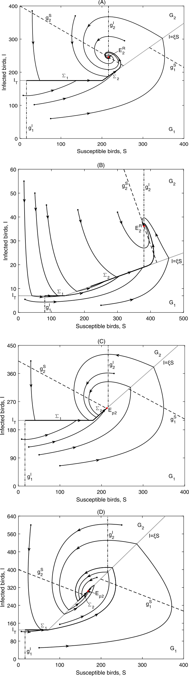
\(E_{2}^{R}\) is globally asymptotically stable in Case B.1: (a) Data 2, \(\xi =0.87, I_{T}=175\), \(\Sigma _{2}=\{(S,I)\in \Omega _{2}: \frac{I_{T}}{\xi }< S< S^{+}\}\); (b) Data 1, \(\xi =0.05, I_{T}=7\), \(\Sigma _{2}=\{(S,I)\in \Omega _{2}: S^{-}< S< S^{+}\}\); \(E_{p2}\) is globally asymptotically stable in Case B.1: (c) Data 2, \(\xi =1.17, I_{T}=210\), \(\Sigma _{2}=\{(S,I)\in \Omega _{2}: \frac{I_{T}}{\xi }< S< S^{+}\}\); (d) Data 2, \(\xi =1.8, I_{T}=130\), \(\Sigma _{2}=\{(S,I)\in \Omega _{2}: S^{-}< S< S^{+}\}\)
-
(i)
-
When \(H_{1}< H_{3}<\frac{I_{T}}{S_{2}^{*}}<H_{2}< \frac{I_{2}^{*}}{S_{2}^{*}}<\frac{I_{T}}{S_{1}^{*}}< \frac{I_{1}^{*}}{S_{1}^{*}}\), we have:
-
(i)
If \(\frac{I_{T}}{S_{2}^{*}}<\xi <\frac{I_{2}^{*}}{S_{2}^{*}}\), then \(E_{2}^{R}\) is a real equilibrium and is globally asymptotically stable; the sliding-mode domain on \(\Omega _{2}\) is \(\Sigma _{2}=\{(S,I)\in \Omega _{2}: \frac{I_{T}}{\xi }< S< S^{+}\}\) when \(\xi < H_{2}\), and \(\Sigma _{2}=\{(S,I)\in \Omega _{2}: S^{-}< S< S^{+}\}\) when \(\xi >H_{2}\), meanwhile \(E_{p2} \notin \Sigma _{2}\subset \Omega _{2}\); as can be seen in Fig. 6(a);
-
(ii)
If \(\frac{I_{2}^{*}}{S_{2}^{*}}<\xi <\frac{I_{T}}{S_{1}^{*}}\), then \(E_{2}^{V}\) is a virtual equilibrium, the sliding-mode domain on \(\Omega _{2}\) is \(\Sigma _{2}=\{(S,I)\in \Omega _{2}: S^{-}< S< S^{+}\}\), meanwhile \(E_{p2} \in \Sigma _{2}\subset \Omega _{2}\) is globally asymptotically stable;
-
(i)
-
When \(H_{1}< H_{3}<\frac{I_{T}}{S_{2}^{*}}<H_{2}<\frac{I_{T}}{S_{1}^{*}}< \frac{I_{2}^{*}}{S_{2}^{*}}<\frac{I_{1}^{*}}{S_{1}^{*}}\), we have that \(E_{2}^{R}\) is a real equilibrium and is globally asymptotically stable; the sliding-mode domain on \(\Omega _{2}\) is \(\Sigma _{2}=\{(S,I)\in \Omega _{2}: \frac{I_{T}}{\xi }< S< S^{+}\}\) when \(\xi < H_{2}\), and \(\Sigma _{2}=\{(S,I)\in \Omega _{2}: S^{-}< S< S^{+}\}\) when \(\xi >H_{2}\), meanwhile \(E_{p2} \notin \Sigma _{2}\subset \Omega _{2}\); as can be seen in Fig. 6(b);
-
When \(H_{1}< H_{3}< H_{2}<\frac{I_{T}}{S_{2}^{*}}<\frac{I_{T}}{S_{1}^{*}}< \frac{I_{2}^{*}}{S_{2}^{*}}<\frac{I_{1}^{*}}{S_{1}^{*}}\), we have that \(E_{2}^{R}\) is a real equilibrium and is globally asymptotically stable; the sliding-mode domain on \(\Omega _{2}\) is \(\Sigma _{2}=\{(S,I)\in \Omega _{2}: S^{-}< S< S^{+}\}\), meanwhile \(E_{p2} \notin \Sigma _{2}\subset \Omega _{2}\);
-
When \(H_{1}< H_{3}< H_{2}<\frac{I_{T}}{S_{2}^{*}}< \frac{I_{2}^{*}}{S_{2}^{*}}<\frac{I_{T}}{S_{1}^{*}}< \frac{I_{1}^{*}}{S_{1}^{*}}\), we have:
-
(i)
If \(\frac{I_{T}}{S_{2}^{*}}<\xi <\frac{I_{2}^{*}}{S_{2}^{*}}\), then \(E_{2}^{R}\) is a real equilibrium and is globally asymptotically stable; the sliding-mode domain on \(\Omega _{2}\) is \(\Sigma _{2}=\{(S,I)\in \Omega _{2}: S^{-}< S< S^{+}\}\), \(E_{p2} \notin \Sigma _{2}\subset \Omega _{2}\);
-
(ii)
If \(\frac{I_{2}^{*}}{S_{2}^{*}}<\xi <\frac{I_{T}}{S_{1}^{*}}\), then \(E_{2}^{V}\) is a virtual equilibrium, the sliding-mode domain on \(\Omega _{2}\) is \(\Sigma _{2}=\{(S,I)\in \Omega _{2}: S^{-}< S< S^{+}\}\), meanwhile \(E_{p2} \in \Sigma _{2}\subset \Omega _{2}\) is globally asymptotically stable; as can be seen in Fig. 6(d).
-
(i)

The solutions of system (1)–(2) in this case will finally stabilize either at \(E_{2}^{R}\) or \(E_{p2}\) with different sliding-mode domains \(\Sigma _{2}\subset \Omega _{2}\), as can be seen in Fig. 6. The disease will persist at an intolerable level or be controlled at the given level. Note that we do not show all the figures, for others are similar with the given ones.
4.3.2 Case B.2: \(I_{2}^{*}< I_{T}< I_{1}^{*}\)
In this case, both \(E_{1}^{V}\) and \(E_{2}^{V}\) are virtual equilibria; \(E_{p1}\) is a pseudoequilibrium if \(\frac{I_{T}}{S_{2}^{*}}<\xi <H_{1}\). For \(\frac{I_{2}^{*}}{S_{2}^{*}}<\frac{I_{T}}{S_{2}^{*}}<H_{3}<H_{1}<H_{2}< \frac{I_{T}}{S_{1}^{*}}<\frac{I_{1}^{*}}{S_{1}^{*}}\) when \(I_{2}^{*}< I_{T}< I_{1}^{*}\), hence, we have the following results.
Theorem 4.2
Suppose \(S_{1}^{*}<\frac{I_{T}}{\xi }<S_{2}^{*}\) and \(I_{2}^{*}< I_{T}< I_{1}^{*}\), we have:
-
(i)
If \(\frac{I_{T}}{S_{2}^{*}}<\xi <H_{1}\), then \(E_{p1} \in \Sigma _{1}\subset \Omega _{1}\) is globally asymptotically stable; there is no sliding mode on \(\Omega _{2}\) when \(\xi < H_{3}\), the sliding-mode domain on \(\Omega _{2}\) is \(\Sigma _{2}=\{(S,I)\in \Omega _{2}: \frac{I_{T}}{\xi }< S< S^{+}\}\) when \(\xi >H_{3}\), meanwhile \(E_{p2} \notin \Sigma _{2}\subset \Omega _{2}\); as can be seen in Fig. 7(a)–(b);
Figure 7 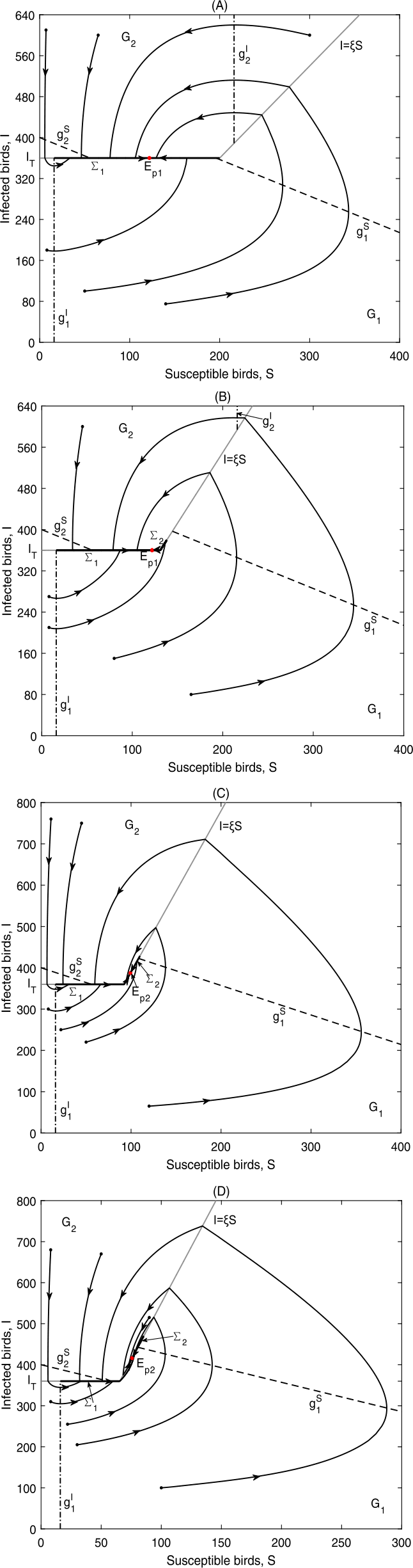
\(E_{p1}\) is globally asymptotically stable in Case B.2: (a) Data 2, \(\xi =1.8, I_{T}=360\), \(\Sigma _{2}\) does not exist; (b) Data 2, \(\xi =2.75, I_{T}=360\), \(\Sigma _{2}=\{(S,I)\in \Omega _{2}: \frac{I_{T}}{\xi }< S< S^{+}\}\); \(E_{p2}\) is globally asymptotically stable in Case B.2: (c) Data 2, \(\xi =3.9, I_{T}=360\), \(\Sigma _{2}=\{(S,I)\in \Omega _{2}: \frac{I_{T}}{\xi }< S< S^{+}\}\); (d) Data 2, \(\xi =5.5, I_{T}=360\), \(\Sigma _{2}=\{(S,I)\in \Omega _{2}: S^{-}< S< S^{+}\}\)
-
(ii)
If \(H_{1}<\xi <\frac{I_{T}}{S_{1}^{*}}\), then \(E_{p1} \notin \Sigma _{1}\subset \Omega _{1}\), the sliding-mode domain on \(\Omega _{2}\) is \(\Sigma _{2}=\{(S,I)\in \Omega _{2}: \frac{I_{T}}{\xi }< S< S^{+}\}\) when \(\xi < H_{2}\), and \(\Sigma _{2}=\{(S,I)\in \Omega _{2}: S^{-}< S< S^{+}\}\) when \(\xi >H_{2}\), meanwhile \(E_{p2} \in \Sigma _{2}\subset \Omega _{2}\) is globally asymptotically stable; as can be seen in Fig. 7(c)–(d).

In this case, the number of infected birds will finally converge to a level equal to the given threshold value, which indicates the disease is controlled from the biological point of view.
4.3.3 Case B.3: \(I_{2}^{*}< I_{1}^{*}< I_{T}\)
In this case, \(E_{1}^{R}\) is a real equilibrium, while \(E_{2}^{V}\) is a virtual equilibrium; \(E_{p1}\) is not a pseudoequilibrium on \(\Omega _{1}\) by Proposition 4.1. We have the following results by Proposition 3.5.
Theorem 4.3
Suppose \(S_{1}^{*}<\frac{I_{T}}{\xi }<S_{2}^{*}\) and \(I_{2}^{*}< I_{1}^{*}< I_{T}\). Then \(E_{1}^{R}\) is globally asymptotically stable, and:
-
When \(\frac{I_{2}^{*}}{S_{2}^{*}}<\frac{I_{T}}{S_{2}^{*}}< \frac{I_{T}}{S_{1}^{*}}<H_{3}<H_{2}<H_{1}\), there is no sliding mode on \(\Omega _{2}\) as can be seen in Fig. 8(a);
Figure 8 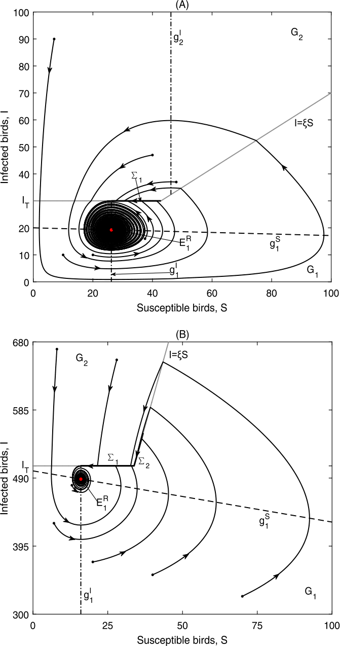
\(E_{1}^{R}\) is globally asymptotically stable in Case B.3: (a) Data 3, \(\xi =0.7, I_{T}=30\), \(\Sigma _{2}\) does not exist; (b) Data 2, \(\xi =15, I_{T}=507\), \(\Sigma _{2}=\{(S,I)\in \Omega _{2}: \frac{I_{T}}{\xi }< S< S^{+}\}\)
-
When \(\frac{I_{2}^{*}}{S_{2}^{*}}<\frac{I_{T}}{S_{2}^{*}}<H_{3}< \frac{I_{T}}{S_{1}^{*}}<H_{2}<H_{1}\), there is no sliding mode on \(\Omega _{2}\) if \(\xi < H_{3}\) and \(\Sigma _{2}=\{(S,I)\in \Omega _{2}: \frac{I_{T}}{\xi }< S< S^{+}\}\) if \(\xi >H_{3}\), meanwhile \(E_{p2} \notin \Sigma _{2}\subset \Omega _{2}\); as can be seen in Fig. 8(b).

As in Case A.3, all solutions will finally stabilize at a level below the infected threshold level \(I_{T}\), as can be seen in Fig. 8, which shows the disease is controlled below a tolerance level.
5 Case C: global dynamics when \(\frac{I_{T}}{\xi }< S_{1}^{*}< S_{2}^{*}\) \((\xi >\frac{I_{T}}{S_{1}^{*}})\)
5.1 Sliding mode on \(\Omega _{1}\) and its dynamics
In this case since \(\frac{I_{T}}{\xi }< S_{1}^{*}\), there does not exist a sliding-mode domain on \(\Omega _{1}\).
5.2 Sliding mode on \(\Omega _{2}\) and its dynamics
As in Case B, the sliding-mode domain on \(\Omega _{2}\) and the conditions for \(E_{p2}\) to be a pseudoequilibrium on \(\Sigma _{2}\subset \Omega _{2}\) are related to the values of ξ and \(I_{T}\), which can be referred to Propositions 3.2 and 3.3. The sliding-mode dynamics on \(\Sigma _{2}\subset \Omega _{2}\) can be represented by system (7).
5.3 Global dynamics
5.3.1 Case C.1: \(I_{T}< I_{2}^{*}< I_{1}^{*}\)
In this situation, \(E_{1}\) is a real equilibrium if \(\xi >\frac{I_{1}^{*}}{S_{1}^{*}}\), whilst \(E_{1}\) is a virtual equilibrium if \(\xi <\frac{I_{1}^{*}}{S_{1}^{*}}\); \(E_{2}\) is a real equilibrium if \(\xi <\frac{I_{2}^{*}}{S_{2}^{*}}\), whilst \(E_{2}\) is a virtual equilibrium if \(\xi >\frac{I_{2}^{*}}{S_{2}^{*}}\). By Proposition 3.5, we have the following results.
Theorem 5.1
Suppose \(S_{1}^{*}< S_{2}^{*}<\frac{I_{T}}{\xi }\) and \(I_{T}< I_{2}^{*}< I_{1}^{*}\). Then the sliding-mode domain on \(\Omega _{2}\) is \(\Sigma _{2}=\{(S,I)\in \Omega _{2}: S^{-}< S< S^{+}\}\) for \(\frac{I_{T}}{S_{1}^{*}}>H_{2}\), and:
-
When \(H_{1}< H_{3}<\frac{I_{T}}{S_{2}^{*}}<\frac{I_{2}^{*}}{S_{2}^{*}}< \frac{I_{T}}{S_{1}^{*}}<\frac{I_{1}^{*}}{S_{1}^{*}}\), one has:
-
(i)
If \(\frac{I_{T}}{S_{1}^{*}}<\xi <\frac{I_{1}^{*}}{S_{1}^{*}}\), both \(E_{1}^{V}\) and \(E_{2}^{V}\) are virtual equilibria; \(E_{p2} \in \Sigma _{2}\subset \Omega _{2}\) is globally asymptotically stable; the figure is similar to Fig. 9(b);
Figure 9 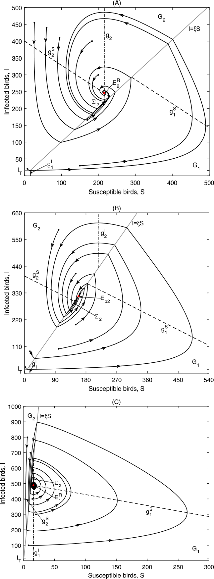
Global dynamics in Case C.1: (a) \(E_{2}^{R}\) is globally asymptotically stable. Data 2, \(\xi =1.01, {I_{T}=16}\); (b) \(E_{p2}\) is globally asymptotically stable. Data 2, \(\xi =2, I_{T}=16\); (c) \(E_{1}^{R}\) is globally asymptotically stable. Data 2, \(\xi =41, I_{T}=16\)
-
(ii)
If \(\xi >\frac{I_{1}^{*}}{S_{1}^{*}}\), \(E_{1}^{R}\) is a real equilibrium, while \(E_{2}^{V}\) is a virtual equilibrium; \(E_{1}^{R}\) is globally asymptotically stable, meanwhile \(E_{p2} \notin \Sigma _{2}\subset \Omega _{2}\); the figure is similar to Fig. 9(c);
-
(i)
-
When \(H_{1}< H_{3}<\frac{I_{T}}{S_{2}^{*}}<\frac{I_{T}}{S_{1}^{*}}< \frac{I_{2}^{*}}{S_{2}^{*}}<\frac{I_{1}^{*}}{S_{1}^{*}}\), one has
-
(i)
If \(\frac{I_{T}}{S_{1}^{*}}<\xi <\frac{I_{2}^{*}}{S_{2}^{*}}\), \(E_{1}^{V}\) is a virtual equilibrium, while \(E_{2}^{R}\) is a real equilibrium; \(E_{2}^{R}\) is globally asymptotically stable, meanwhile \(E_{p2} \notin \Sigma _{2}\subset \Omega _{2}\) as can be seen in Fig. 9(a);
-
(ii)
If \(\frac{I_{2}^{*}}{S_{2}^{*}}<\xi <\frac{I_{1}^{*}}{S_{1}^{*}}\), both \(E_{1}^{V}\) and \(E_{2}^{V}\) are virtual equilibria; \(E_{p2} \in \Sigma _{2}\subset \Omega _{2}\) is globally asymptotically stable as can be seen in Fig. 9(b);
-
(iii)
If \(\xi >\frac{I_{1}^{*}}{S_{1}^{*}}\), \(E_{1}^{R}\) is a real equilibrium, while \(E_{2}^{V}\) is a virtual equilibrium; \(E_{1}^{R}\) is globally asymptotically stable, meanwhile \(E_{p2} \notin \Sigma _{2}\subset \Omega _{2}\) as can be seen in Fig. 9(c).
-
(i)

In this case, all solutions of system (1)–(2) rely greatly on the combinations of \(I_{T}\) and ξ. The solutions should converge to \(E_{2}^{R}\), \(E_{p2}\) or \(E_{1}^{R}\) as can be seen in Fig. 9, which then leads to different control outcomes. Therefore an efficient threshold policy is essential by driving the number of infected birds below a given level or at a tolerance level.
5.3.2 Case C.2: \(I_{2}^{*}< I_{T}< I_{1}^{*}\)
In this case, for \(\frac{I_{2}^{*}}{S_{2}^{*}}<\frac{I_{T}}{S_{2}^{*}}<H_{3}<H_{1}<H_{2}< \frac{I_{T}}{S_{1}^{*}}<\frac{I_{1}^{*}}{S_{1}^{*}}\) and \(\xi >\frac{I_{T}}{S_{1}^{*}}\), then \(\xi >\frac{I_{2}^{*}}{S_{2}^{*}}\) and \(E_{2}\) is a virtual equilibrium, denoted by \(E_{2}^{V}\); \(E_{1}\) is a real equilibrium if \(\xi >\frac{I_{1}^{*}}{S_{1}^{*}}\), whilst \(E_{1}\) is a virtual equilibrium if \(\xi <\frac{I_{1}^{*}}{S_{1}^{*}}\).
Theorem 5.2
Suppose \(S_{1}^{*}< S_{2}^{*}<\frac{I_{T}}{\xi }\) and \(I_{2}^{*}< I_{T}< I_{1}^{*}\). Then the sliding-mode domain on \(\Omega _{2}\) is \(\Sigma _{2}=\{(S,I)\in \Omega _{2}: S^{-}< S< S^{+}\}\) for \(H_{2}<\frac{I_{T}}{S_{1}^{*}}\), and:
-
(i)
If \(\frac{I_{T}}{S_{1}^{*}}<\xi <\frac{I_{1}^{*}}{S_{1}^{*}}\), \(E_{1}^{V}\) is a virtual equilibrium. \(E_{p2} \in \Sigma _{2}\subset \Omega _{2}\) is globally asymptotically stable as can be seen in Fig. 10(a);
Figure 10 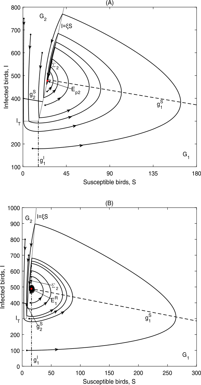
Global dynamics in Case C.2: (a) \(E_{p2}\) is globally asymptotically stable. Data 2, \(\xi =18.8, {I_{T}=300}\); (b) \(E_{1}^{R}\) is globally asymptotically stable. Data 2, \(\xi =41, I_{T}=300\)
-
(ii)
If \(\xi >\frac{I_{1}^{*}}{S_{1}^{*}}\), \(E_{1}^{R}\) is a real equilibrium and is globally asymptotically stable, meanwhile \(E_{p2} \notin \Sigma _{2}\subset \Omega _{2}\) as can be seen in Fig. 10(b).

As can be seen in Fig. 10, all solutions of the system will finally stabilize at either \(E_{p2}\) or \(E_{1}^{R}\), the level equal to or below the given threshold level, and then the influenza is controlled below or at a tolerance level.
5.3.3 Case C.3: \(I_{2}^{*}< I_{1}^{*}< I_{T}\)
In this case, \(E_{1}^{R}\) is a real equilibrium, \(E_{2}^{V}\) is a virtual equilibrium. By Proposition 3.5, we have the following result.
Theorem 5.3
Suppose \(S_{1}^{*}< S_{2}^{*}<\frac{I_{T}}{\xi }\) and \(I_{2}^{*}< I_{1}^{*}< I_{T}\), then \(E_{1}^{R}\) is globally asymptotically stable, and for \(\frac{I_{1}^{*}}{S_{1}^{*}}<\frac{I_{T}}{S_{1}^{*}}\) we have:
-
When \(\frac{I_{2}^{*}}{S_{2}^{*}}<\frac{I_{T}}{S_{2}^{*}}< \frac{I_{T}}{S_{1}^{*}}<H_{3}<H_{2}<H_{1}\), there does not exist a sliding-mode domain if \(\xi < H_{3}\), the sliding-mode domain on \(\Omega _{2}\) is \(\Sigma _{2}=\{(S,I)\in \Omega _{2}: \frac{I_{T}}{\xi }< S< S^{+}\}\) if \(H_{3}<\xi <H_{2}\), and \(\Sigma _{2}=\{(S,I)\in \Omega _{2}: S^{-}< S< S^{+}\}\) if \(\xi >H_{2}\), meanwhile \(E_{p2} \notin \Sigma _{2}\subset \Omega _{2}\) as can be seen in Fig. 11(a)–(b);
Figure 11 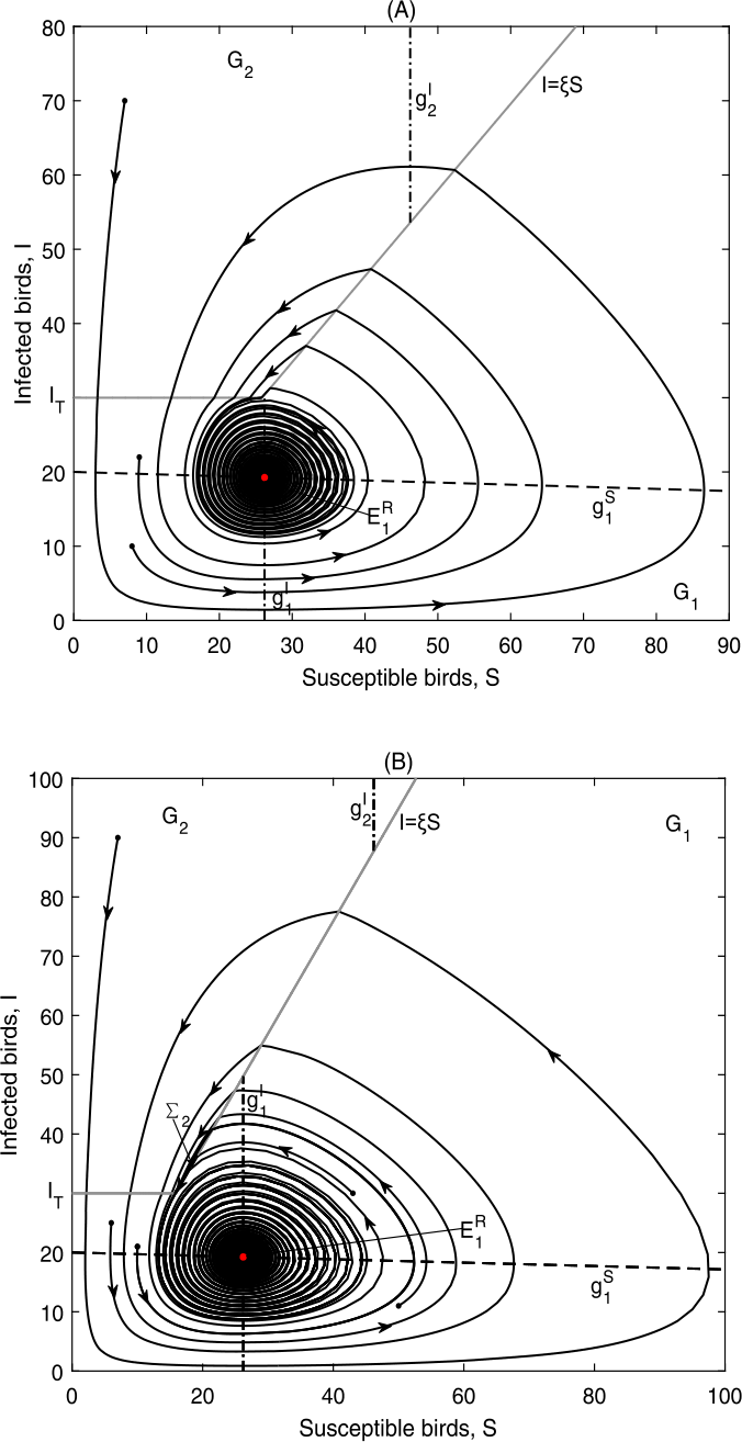
\(E_{1}^{R}\) is globally asymptotically stable in Case C.3: (a) Data 3, \(\xi =1.16, I_{T}=30\). \(\Sigma _{2}\) does not exist; (b) Data 3, \(\xi =1.9, I_{T}=30\), \(\Sigma _{2}=\{(S,I)\in \Omega _{2}: \frac{I_{T}}{\xi }< S< S^{+}\}\)
-
When \(\frac{I_{2}^{*}}{S_{2}^{*}}<\frac{I_{T}}{S_{2}^{*}}<H_{3}< \frac{I_{T}}{S_{1}^{*}}<H_{2}<H_{1}\), the sliding-mode domain on \(\Omega _{2}\) is \(\Sigma _{2}=\{(S,I)\in \Omega _{2}: \frac{I_{T}}{\xi }< S< S^{+}\}\) if \(\xi < H_{2}\), and \(\Sigma _{2}=\{(S,I)\in \Omega _{2}: S^{-}< S< S^{+}\}\) if \(\xi >H_{2}\), meanwhile \(E_{p2} \notin \Sigma _{2}\subset \Omega _{2}\); the figures are similar to Fig. 11(a)–(b).

The outcomes in this case achieve our objective as shown in Fig. 11, that is, to drive the number of infected birds to a level below the tolerance level. We could choose the corresponding threshold values in practice.
6 Conclusion and discussion
In this work, we proposed and analyzed an avian-only Filippov model, which is governed by nonlinear ordinary differential equations with discontinuous right-hand sides and a nonsmooth separation line. On the one hand, it is generally impossible to completely depopulate the infected birds, nor it is economically or biologically feasible. So when carrying out control strategies, the objective is to drive the number of infected birds to a tolerance or available level. On the other hand, when the interaction ratio of the numbers of infected and susceptible birds is below a ratio threshold value ξ, in order to maximize the economic profits, more effort can be saved by taking no control measures. In Sects. 3–5, it is shown that the solutions of system (1)–(2) will finally stabilize at either one of the two endemic equilibria in each subregion or the sliding equilibria on the two sliding modes. The results indicate that we can choose a suitable tolerance threshold \(I_{T}\) and/or a suitable ratio threshold ξ such that system (1)–(2) finally approaches \(E_{1}\) in \(G_{1}\) or a sliding equilibrium \(E_{pi}\) on \(\Sigma _{i}\subset \Omega _{i}, i=1,2\), and then our objective, that is, inhibiting the infection or stabilizing the infection to a desirable level, is obtained. The main analytical results are summarized in Table 2, with the following biological implications.
-
(I)
The system (1)–(2) has a unique globally asymptotically stable equilibrium \(E_{1}^{R}\), as illustrated in Figs. 5, 8, 9(c), 10(b), 11. The number of infected birds will finally stabilize at a level below the given threshold. Hence, in this situation, the influenza could be controlled below a given level in spite of a small endemic with size \(E_{1}^{R}\). In practice, these choices of threshold values are preferable.
-
(II)
The system (1)–(2) has a unique globally asymptotically stable equilibrium \(E_{2}^{R}\), as can be seen in Figs. 3, 6(a)–(b), 9(a). For these choices of threshold levels, the number of infected birds will converge to a high level above the threshold values, and then the avian influenza may be out of control by persisting at an intolerable level \(E_{2}^{R}\).
-
(III)
There is a globally asymptotically stable pseudoequilibrium \(E_{p1}\) or \(E_{p2}\). So the number of infected birds will eventually approach the given threshold values, as can be seen in Figs. 6(c)–(d), 7, 9(b), 10(a). The influenza is finally controlled at a tolerance level.
Note that our objective is to maintain the number of infected birds not exceeding a desired level. The analytical results show that the choice of the infected threshold value \(I_{T}\) and the ratio threshold ξ is of great significance to lead the number of the infected birds to an acceptable level. For Cases (I) and (III), our control objective can be achieved since the eventual number of the infected birds is equal to or below the given threshold levels. However, the number of the infected birds will be above the separation line eventually in Case (II), which is not our desire since tremendous economic damage will be caused. The findings could be beneficial to decide whether and when to take control strategies based on these two threshold values.
The threshold policy adopted by Chong et al. [25] treats the infected birds as an index. However, when the number of infected birds is relatively small compared to the number of susceptible birds, economic considerations may be more important than the disease control. Hence, a threshold policy considering both the number of infected birds and the interaction ratio of the numbers of infected and susceptible birds may be more realistic from the economical point of view. On the other hand, compared with the model proposed by Chong et al. [25] (\(\xi =0\) in system (1)–(2) with constant growth for the susceptible birds), we find that if the values of \(I_{T}\) and/or ξ are chosen to satisfy \(S_{2}^{*}<\frac{I_{T}}{\xi }\) or \(I_{T}>I_{1}^{*}\), then both models present the same results, that is, the disease persists at the level of \(E_{2}\) when \(I_{T}< I_{2}^{*}\), the number of infected birds stays at the available level \(E_{p1}\) when \(I_{2}^{*}< I_{T}< I_{1}^{*}\), and the influenza is totally in control by stabilizing at \(E_{1}\) when \(I_{T}>I_{1}^{*}\). However, when the number of susceptible and/or infected birds is large enough, system (1)–(2) shows more complex dynamics. For example, in Case C.1 when \(\frac{I_{T}}{\xi }< S_{1}^{*}< S_{2}^{*}\) and \(I_{T}< I_{2}^{*}\), the solutions could converge to \(E_{2}^{R}, E_{p2}\) or \(E_{1}^{R}\), resulting in different control outcomes, which shows the importance of the number of susceptible birds and the interaction ratio of the infected and susceptible birds in disease control.
Also, in [38] and our previous work [9], the authors considered a two-threshold policy in combating avian influenza. That is, culling of infected and/or susceptible birds depends on whether the number of infected (susceptible) birds exceeds the infected (susceptible) threshold level or not. The results show that if the susceptible threshold level is chosen to be large enough while the infected threshold level is chosen to be small enough, then the disease may persist at an intolerable level. While system (1)–(2) in this case indicates that the disease could be controlled to below the tolerance level. Hence taking the interaction ratio of the infected and susceptible birds into consideration may be of some importance. Therefore, the avian-only model with a nonsmooth separation line proposed in this work may provide some new threshold policies in avian influenza control.
The theoretical results obtained in this work show that by choosing an appropriate threshold policy with a suitable tolerance threshold \(I_{T}\) and/or a suitable ratio threshold ξ, we can finally drive the influenza below or to be equal to the given tolerance level. It is worth noting that depopulation of susceptible and/or infected birds can still be triggered to stop the infection from progressing to an intolerable pandemic. Therefore an effective and efficient threshold policy is essential to control the influenza by driving the number of infected birds below or to a chosen level.
Availability of data and materials
Not applicable.
References
Alexander, J.D.: An overview of the epidemiology of avian influenza. Vaccine 25, 5637–5644 (2007)
Alexander, J.D.: A review of avian influenza in different bird species. Vet. Microbiol. 74, 3–13 (2000)
Peiris, J.S., de Jong, M.D., Guan, Y.: Avian influenza virus (H5N1): a threat to human health. Clin. Microbiol. Rev. 20, 243–267 (2007)
Smith, G.J., Bahl, J., Vijaykrishna, D., Zhang, J., Poon, L.M., Chen, H., et al.: Dating the emergence of pandemic influenza viruses. Proc. Natl. Acad. Sci. 106, 11709–11712 (2009)
Zilberman, D., Otte, J., Roland-Host, D., Pfeiffer, D.: The cost of saving a statistical life: a case for influenza prevention and control. Nat. Resour. Manag. Policy 36, 135–141 (2012)
Li, Q., Zhou, L., Zhou, M., Chen, Z., Li, F., Wu, H., et al.: Epidemiology of human infections with avian influenza A(H7N9) virus in China. N. Engl. J. Med. 370(6), 520–532 (2014)
He, Y., Liu, P., Tang, S., Chen, Y., Pei, E., Zhao, B., et al.: Live poultry market closure and control of avian influenza A(H7N9), Shanghai, China. Emerg. Infect. Dis. 20(9), 1565–1566 (2014)
Perez, D.R., Garcia-Sastre, A.: H5N1, a wealth of knowledge to improve pandemic preparedness. Virus Res. 178, 1–2 (2013)
Yang, Y., Wang, L.: Global dynamics and rich sliding motion in an avian-only Filippov system in combating avian influenza. Int. J. Bifurc. Chaos 30(1), 2050008 (2020)
Avian Influenza-Questions & Answers Tech. Rep.: Animal Production and Health Division. http://www.fao.org/avianflu/en/qanda.html#7 (2018)
Mu, R., Yang, Y.: Global dynamics of an avian influenza A(H7N9) epidemic model with latent period and nonlinear recovery rate. Comput. Math. Methods Med. 2018, 7321694 (2018)
Liu, S., Ruan, S., Zhang, X.: Nonlinear dynamics of avian influenza epidemic models. Math. Biosci. 283, 118–135 (2017)
Yang, X., Li, X.: Finite-time stability of linear non-autonomous systems with time-varying delays. Adv. Differ. Equ. 2018, 101 (2018)
Hu, J., Sui, G., Lv, X., Li, X.: Fixed-time control of delayed neural networks with impulsive perturbations. Nonlinear Anal., Model. Control 23(6), 904–920 (2018)
Yang, D., Li, X., Shen, J., Zhou, Z.: State-dependent switching control of delayed switched systems with stable and unstable modes. Math. Methods Appl. Sci. 41(16), 6968–6983 (2018)
Li, X., Yang, X., Huang, T.: Persistence of delayed cooperative models: impulsive control method. Appl. Math. Comput. 342, 130–146 (2019)
Ma, X., Wang, W.: A discrete model of avian influenza with seasonal reproduction and transmission. J. Biol. Dyn. 4, 296–314 (2010)
Andronicoa, A., Courcoulb, A., Bronnerc, A., Scoizecd, A., Lebouquin-Leneveuet, S., Guinat, C., et al.: Highly pathogenic avian influenza H5N8 in South-West France 2016–2017: a modeling study of control strategies. Epidemics 28, 100340 (2019)
Yang, X., Li, X., Xi, Q., Duan, P.: Review of stability and stabilization for impulsive delayed systems. Math. Biosci. Eng. 15(6), 1495–1515 (2018)
Mu, R., Wei, A., Yang, Y.: Global dynamics and sliding motion in A(H7N9) epidemic models with limited resources and Filippov control. J. Math. Anal. Appl. 477(2), 1296–1317 (2019)
Zhu, C., Li, X., Cao, J.: Finite-time H-infinity dynamic output feedback control for nonlinear impulsive switched systems. Nonlinear Anal. Hybrid Syst. 39, 100975 (2021)
Xiao, Y., Xu, X., Tang, S.: Sliding mode control of outbreaks of emerging infectious diseases. Bull. Math. Biol. 74, 2403–2422 (2012)
Zhou, W., Xiao, Y., Cheke, R.: A threshold policy to interrupt transmission of West Nile virus to birds. Appl. Math. Model. 40(19–20), 8794–8809 (2016)
Bolzoni, L., Della Marca, R., Groppi, M.: Dynamics of a metapopulation epidemic model with localized culling. Discrete Contin. Dyn. Syst., Ser. B 25(6), 2307–2330 (2020)
Chong, N., Smith, R.: Modelling avian influenza using Filippov systems to determine culling of infected birds and quarantine. Nonlinear Anal., Real World Appl. 24, 196–218 (2015)
Li, W.X., Huang, L.H., Wang, J.F.: Dynamic analysis of discontinuous plant disease models with a non-smooth separation line. Nonlinear Dyn. 99, 1675–1697 (2020)
Zhang, J., Jin, Z., Sun, G., Sun, X., Wang, Y., Huang, B.: Determination of original infection source of H7N9 avian influenza by dynamical model. Sci. Rep. 4, 1–16 (2014)
Rappole, J.H., Hubalek, Z.: Migratory birds and West Nile virus. J. Appl. Microbiol. 94, 47S–58S (2003)
Filippov, A.: Differential Equations with Discontinuous Righthand Sides. Kluwer Academic, Dordrecht (1988)
Yang, Y., Zhang, T.: Modeling plant virus propagation with Filippov control. Adv. Differ. Equ. 2020, 465 (2020)
Kuznetsov, Y.A., Rinaldi, S., Gragnani, A.: One parameter bifurcations in planar Filippov systems. Int. J. Bifurc. Chaos 13, 2157–2188 (2003)
Li, X., Caraballo, T., Rakkiyappan, R., Han, X.: On the stability of impulsive functional differential equations with infinite delays. Math. Methods Appl. Sci. 38(14), 3130–3140 (2015)
Li, X., Bohner, M.: An impulsive delay differential inequality and applications. Comput. Math. Appl. 64(6), 1875–1881 (2012)
Utkin, V.I., Guldner, J., Shi, J.X.: Sliding Mode Control in Electro-Mechanical System, 2nd edn. Taylor & Francis, London (2009)
van den Driessche, P., Watmough, J.: Reproduction numbers and sub-threshold endemic equilibria for compartmental models of disease transmission. Math. Biosci. 180, 29–48 (2002)
Leine, R.I.: Bifurcations in Discontinuous Mechanical Systems of Filippov-Type. The Universiteitsdrukkerij TU Eindhoven, The Netherlands (2000)
Leine, R.I., van Campen, D.H., van de Vrande, B.L.: Bifurcations in nonlinear discontinuous systems. Nonlinear Dyn. 23, 105–164 (2000)
Chong, N., Dionne, B., Smith, R.: An avian-only Filippov model incorporating culling of both susceptible and infected birds in combating avian influenza. J. Math. Biol. 73, 751–784 (2016)
Acknowledgements
Not applicable.
Funding
National Natural Science Foundation of China (NSFC 11401349) and the Foundation for Outstanding Young Scientist in Shandong Province (BS2014SF008).
Author information
Authors and Affiliations
Contributions
In this research work, YY contributed to analysis and manuscript preparation. JW performed the numerical simulations. All authors read and approved the final manuscript.
Corresponding author
Ethics declarations
Competing interests
The authors declare that they have no competing interests.
Rights and permissions
Open Access This article is licensed under a Creative Commons Attribution 4.0 International License, which permits use, sharing, adaptation, distribution and reproduction in any medium or format, as long as you give appropriate credit to the original author(s) and the source, provide a link to the Creative Commons licence, and indicate if changes were made. The images or other third party material in this article are included in the article’s Creative Commons licence, unless indicated otherwise in a credit line to the material. If material is not included in the article’s Creative Commons licence and your intended use is not permitted by statutory regulation or exceeds the permitted use, you will need to obtain permission directly from the copyright holder. To view a copy of this licence, visit http://creativecommons.org/licenses/by/4.0/.
About this article

Cite this article
Yang, Y., Wang, J. Rich dynamics of a Filippov avian-only influenza model with a nonsmooth separation line. Adv Differ Equ 2021, 212 (2021). https://doi.org/10.1186/s13662-021-03375-z
Received:
Accepted:
Published:
DOI: https://doi.org/10.1186/s13662-021-03375-z