Semi-supervised semantic segmentation in Earth Observation: the MiniFrance suite, dataset analysis and multi-task network study

Abstract

The development of semi-supervised learning techniques is essential to enhance the generalization capacities of machine learning algorithms. Indeed, raw image data are abundant while labels are scarce, therefore it is crucial to leverage unlabeled inputs to build better models. The availability of large databases have been key for the development of learning algorithms with high level performance. Despite the major role of machine learning in Earth Observation to derive products such as land cover maps, datasets in the field are still limited, either because of modest surface coverage, lack of variety of scenes or restricted classes to identify. We introduce a novel large-scale dataset for semi-supervised semantic segmentation in Earth Observation, the MiniFrance suite. MiniFrance has several unprecedented properties: it is large-scale, containing over 2000 very high resolution aerial images, accounting for more than 200 billions samples (pixels); it is varied, covering 16 conurbations in France, with various climates, different landscapes, and urban as well as countryside scenes; and it is challenging, considering land use classes with high-level semantics. Nevertheless, the most distinctive quality of MiniFrance is being the only dataset in the field especially designed for semi-supervised learning: it contains labeled and unlabeled images in its training partition, which reproduces a life-like scenario. Along with this dataset, we present tools for data representativeness analysis in terms of appearance similarity and a thorough study of MiniFrance data, demonstrating that it is suitable for learning and generalizes well in a semi-supervised setting. Finally, we present semi-supervised deep architectures based on multi-task learning and the first experiments on MiniFrance. These results will serve as baselines for future work on semi-supervised learning over the MiniFrance dataset. The Minifrance suite and related semi-supervised networks will be publicly available to promote semi-supervised works in Earth Observation.

1 Introduction

Earth Observation (EO) data analysis plays a major role on the way we understand our planet and its dynamics. Indeed, the ever-growing amount of remote sensing imagery data in the last decades has allowed new developments in the fields of ecology, urban planning or natural disaster response (Runting et al. 2020), and will certainly be crucial on the battle against climate change.

In recent years, deep learning techniques—and the significant growth of computing power jointly with massive amounts of (labeled) data available—have transformed the fields of machine learning and computer vision. Moreover, remote sensing imagery has not been the exception since several state-of-the-art methods for classification, object detection and image segmentation have proved to be most effective in this kind of data too (Audebert et al. 2018; Maggiori et al. 2017; Zhu et al. 2017).

Unfortunately, most of the machine learning algorithms—and particularly, deep learning methods—developed to date rely heavily on the availability of annotated image databases. Labeled data is hard to obtain, requiring too much effort and time, while raw data—without labels—is abundant, especially in remote sensing where satellites generate data continuously (e.g., Copernicus Sentinels provide up to 5 day coverage of the Earth). Because of this, we are convinced that semi-supervised methods—which leverage unlabeled data to help on the learning process—will be essential to push further the generalization capacities of the models.

To this end, we propose the first large-scale dataset for semi-supervised semantic segmentation in the field: the MiniFrance dataset. It will encourage research on semi-supervised methods and will provide a common and reliable benchmark to new algorithms, just as ImageNet (Deng et al. 2009) did on traditional computer vision a decade ago. Along with the MiniFrance suite, we conduct a thorough analysis of data in terms of representativeness to define a convenient partition for semi-supervision and we present semi-supervised methods for semantic segmentation, based on multi-task learning, that show the effectiveness of semi-supervised learning and will serve as baselines for future work on this dataset. For this reason, the MiniFrance suite and related semi-supervised networks will be made publicly available.

Thus, our contributions are threefold:

• We introduce MiniFrance a new large scale dataset for semi-supervised semantic segmentation in Earth Observation.¹

• We define techniques for prior analysis of the representativeness of datasets for training and deploying models which help evaluate the need for domain adaptation.

• We show the benefits of semi-supervised learning strategies to improve semantic segmentation:

  • In particular, we propose a new loss function for unsupervised or semi-supervised image segmentation;

  • we report an extensive study of semi-supervised learning with different losses and multi-task architectures.

On account of this, we start by exploring some related work in Sect. 2. Section 3 describes the MiniFrance suite in details, while Sect. 4 introduces some tools to analyze data representativeness and appearance similarity in multi-location datasets. This allows us to get meaningful insight about the MiniFrance dataset and to define a suitable partition—labeled training, unlabeled training and testing—to perform semi-supervised learning. We introduce our semi-supervised strategies in Sect. 5, including neural network architectures and unsupervised losses to consider in a multi-task learning scheme. We then present in Sect. 6 the analysis and experimental study of semi-supervised learning over the MiniFrance dataset. They provide deeper understanding about semi-supervised learning and show the interest of the development of these techniques, that use unlabeled data to enhance the learning process, improving the generalization capacities of the models. These results will also serve as baselines for future work on semi-supervised learning over the MiniFrance dataset.

2 Related work

Since we aim to perform semantic segmentation on remote sensing data using deep semi-supervised neural networks, we discuss here the related work on semantic segmentation, EO datasets, and semi-supervised learning.

2.1 Semantic segmentation

Semantic segmentation consists in the process of assigning a class label to every pixel on an image. It is a relevant task in computer vision because it implies understanding the context of a scene or an image which might be crucial for some applications, like autonomous driving or medical image diagnostics.

If in the last decade convolutional neural networks (CNNs) became the state-of-the-art to perform image classification and object detection, the breakthrough of fully convolutional networks (Long et al. 2015) (FCNs) revolutionized the way of obtaining dense pixel-wise predictions. This kind of architectures takes advantage of CNNs replacing the last fully connected layers by convolutional ones, obtaining dense prediction maps. Today, state-of-the-art semantic segmentation networks, from SegNet (Badrinarayanan et al. 2017) and U-Net (Ronneberger et al. 2015) to PSPNet (Zhao et al. 2017) or DeepLab (Chen et al. 2017), all inherit from the FCN paradigm. A comprehensive review can be found in Minaee et al. (2020).

Processing of EO data has also greatly benefited from these techniques which now define the state-of-the-art in the field. Semantic segmentation is one of the main tasks in remote sensing since it provide pixel-wise classification that corresponds to land cover or land use maps (i.e. the most popular EO products). After seminal works for road detection (Mnih and Hinton 2010), generic multi-class segmentation was soon tackled with CNNs and FCNs (Paisitkriangkrai et al. 2015; Campos-Taberner et al. 2016; Audebert et al. 2018; Rey et al. 2017), until latest developments which result in global cover maps of a continent or the entire planet (Demuzere et al. 2019). With respect to these approaches, our work aims at leveraging also unlabeled data for estimating the classification model.

2.2 Datasets for Earth Observation

The tremendous progress of computer vision—where machine learning is applied on images—in the last decades would not have been possible without the development of large public datasets, such as ImageNet (Deng et al. 2009), COCO (Lin et al. 2014) or Cityscapes (Cordts et al. 2016) for learning on visual data. These datasets provide the means to compare models, and to test their scalability and reliability. They are the key to improve performance of algorithms and push research limits further.

In view of the above, the remote sensing community has also published several datasets for different tasks in order to encourage the research in the field. Table 1 describes the main initiatives.

Table 1 Earth Observation datasets summary

If some of the datasets mentioned above already take into account multiple locations, most are limited to urban scenes only and they are devoted to a single class (such as buildings) or to land cover (and not land use) classes. Land cover refers to the ground surface coverage: vegetation, urban infrastructure, water, etc; while land use indicates the purpose the land serves: urban, industrial buildings, agriculture, etc. The second is more interesting to analyze, because it provides further information about human activity in a given area, however extracting this information from images only remains a major challenge (Fisher et al. 2005). MiniFrance, however, offers scenes from urban and countryside zones, with land-use, high semantic level of classes and covers a vast surface (larger than other datasets at very high resolution—VHR), with aerial images at a sub-meter resolution, including $\sim 150$ GB of data.

Furthermore, all the aforementioned datasets were designed for fully supervised learning, which does not correspond to the real practical case where huge amounts of imagery are available, but only a few images come with some labeled regions. MiniFrance is the first dataset that includes labeled and unlabeled data that can be used in training phases, thus recreating a realistic scenario.

2.3 Semi-supervised learning

Semi-supervised learning (Chapelle et al. 2006) refers to all the techniques that are halfway between supervised and unsupervised learning. In these settings, available data can be divided in two parts: a labeled set where raw data and its corresponding target are provided, and an unlabeled set for which only raw data are available. The key idea behind semi-supervised learning is to learn a representation function (that maps a data point to its target) from labeled data as in the supervised approach, but using the available unlabeled data to leverage information about structure of these data to help the learning process. This is a much realistic and compelling approach than supervised learning, since in real-life applications annotated data is difficult to procure—even harder in the context of semantic segmentation, since one needs pixel-wise labels—while raw data is plentiful.

Semi-supervised methods for semantic segmentation in deep learning have been developed in the last years, but mostly in the form of weakly supervision: from scribbles (Maggiolo et al. 2018; Durand et al. 2017) bounding boxes (Khoreva et al. 2017; Papandreou et al. 2015) and image-level annotations (Papandreou et al. 2015) to obtain dense, pixel-wise predictions. Pseudo-labels (Lee 2013) can also be used to address the semi-supervised problem (Chen et al. 2020), propagating labels from annotated examples through non-annotated ones, according to a confidence criterion, to artificially enlarge available training data. Other works include unlabeled data during training in a generative adversarial network framework (Souly et al. 2017; Hung et al. 2018). The method in Kalluri et al. (2019) is similar to our settings in the way unlabeled images are exploited, but targets a domain adaptation task and requires an alignment of the features from multiple domains through an entropy module.

Semi-supervised methods for remote sensing applications have also been studied in the last years.  Xia et al. (2013) presents a feature extraction method based on principal component analysis that uses labeled and unlabeled data, Tuia et al. (2014) and Hong et al. (2019) leverage unlabeled examples to achieve manifold alignment of data coming from different modalities. More recently, deep learning based approaches have leveraged weakly labeled data for different purposes. Nivaggioli and Randrianarivo (2019) and Schmitt et al. (2020) use weak supervision for land cover classification. Zhang et al. (2020) uses open and incomplete available data (OpenStreetMap—OSM) to generate maps of a large-scale zone. Bonafilia et al. (2019) also uses OSM data as weak labels for building extraction. Le et al. (2019) performs weakly supervised semantic segmentation to detect penguin colonies on the Antarctic.

Fewer are the works that, like us, exploit completely unlabeled examples during the training process. Tao et al. (2017) uses labeled and unlabeled data in an alternating training process to perform semi-supervised semantic segmentation of remote sensing images, while Zhu et al. (2019) leverages unlabeled data for domain adaptation purposes using an adversarial training strategy.

Conversely to previous works, we aim here to leverage completely unlabeled images and fully annotated ones to jointly train deep neural networks with an adapted loss and architecture, in a multi-task learning framework, training one unique model end-to-end, for semi-supervised semantic segmentation of aerial images.

3 The MiniFrance suite

Considering the limitations of current Earth Observation (EO) datasets emphasized in Sect. 2.2, we propose a new large-scale benchmark suite for semi-supervised semantic segmentation: MiniFrance. As in real life EO applications, it comprises both labeled and unlabeled imagery for developing and training algorithms. To our knowledge, this is the first dataset designed for benchmarking semi-supervised learning in the field. Moreover, it consists of a variety of classes on several locations with different appearances: this allows to push further the generalization capacities of the models.

3.1 MiniFrance

It consists of data corresponding to 16 conurbations and their surroundings from different regions in France (see Fig. 1; Table 2). It includes urban and countryside scenes: residential areas, industrial and commercial zones but also fields, forests, sea-shore or low mountains.

Fig. 1

Dataset overview

Table 2 List of cities in MiniFrance and split details (Color figure online)

MiniFrance gathers data from two sources:

• Open data VHR aerial images from the French National Institute of Geographical and Forest Information (IGN) BD ORTHO database.²

  They are provided as RGB tiles of size 10,000 px $\times$ 10,000 px at a resolution of 50 cm/px, namely 25 km$^2$ per tile. Images included in this dataset were acquired between 2012 and 2014.

• Labeled class-reference from the UrbanAtlas 2012 database. Original data are openly available as vector images (i.e. containing polygon annotations) at the European Copernicus program website.³ Using the georeferenced data available in the BD ORTHO, we have made rasters of these images that geographically match the VHR tiles from the BD ORTHO. We consider 14 land-use classes (see Table 3), corresponding to the second level of the semantic hierarchy defined by UrbanAtlas (Montero et al. 2014). For this reason, some of them might not be present in the regions considered for MiniFrance and they are colored in gray in Table 3.

  Table 3 Land use classes available in MiniFrance

Collecting data from different sources brings some burden that must be considered. Land use maps from UrbanAtlas are obtained through a semi-automatic process and thus they are not 100% accurate (Lefebvre et al. 2016), besides polygon annotations might not match 50 cm/px resolution images precisely. Moreover, additional errors might come from the fact that image and ground-truth may not correspond to the same year. Nonetheless, MiniFrance has several peculiar, unprecedented properties that we detail now.

Large-scale MiniFrance is a very large-scale dataset. It contains a total of 2121 aerial images of size 10,000 px $\times$ 10,000 px at 50 cm/px resolution. In terms of ground coverage, with 53,000 km$^2$ it is 12 times larger than DeepGlobe and larger than xBD, among the datasets of similar resolution.

Rich and varied MiniFrance includes aerial images of 16 conurbations and their surroundings from different regions with various climates and landscapes (Mediterranean, oceanic and mountainous) in France. Introducing various locations leads to various appearances for the same class (buildings look different, vegetation is not the same and so on). Moreover, it combines urban centers, rural areas and large forest scenes. With respect to remote sensing datasets like ISPRS Vaihingen and Potsdam, it offers much more variety, as already observed in Sect. 2.2. We propose an experimental comparison between MiniFrance and Vaihingen in Sect. 6.1.

High semantic level of classes MiniFrance considers 14 land-use classes, which is more than most of the datasets exposed in Sect. 2.2. However, these classes have higher semantics: to identify an “urban area” an algorithm must be able to find several houses or buildings together, same to classify a forest. It is much easier to only consider classes at an object level (cars, buildings, trees, etc). Moreover, land-use classes are hard to learn, even for humans: how to distinguish pastures  from artificial non-agricultural vegetated areas  in Fig. 2?

Fig. 2

Some samples of MiniFrance dataset on different localizations. Images (up) and their associated ground-truth (down). From left to right: Nice, Rennes and Vannes

Underlying domain adaptation problem Since train and test sets were split by city—instead of excluding random tiles from all the zones—algorithms developed on MiniFrance must address the underlying problem of domain adaptation. The appearance of classes might vary considerably from one city to another. Architecture is not the same, agriculture may change, etc. In Fig. 2 we observe that urban fabric  does not look alike between the three exposed images.

Designed for semi-supervised semantic segmentation To our knowledge, this is the first dataset specifically designed for semi-supervised learning strategies. Indeed, our training split includes labeled (two cities) and unlabeled images (six ones) while algorithms can be tested on the eight remaining cities. With such a proportion of unlabeled examples, this fosters the development of new methods to leverage them. Moreover, these methods are likely to be easily transferred to lifelike scenarios and to have better generalization properties by design. Table 2 presents our training—labeled and unlabeled images—and testing splits.

3.2 Tiny MiniFrance

To allow prototyping new algorithms with fast processing and validation times we also introduce tinyMiniFrance (tMF), a small, computationally tractable version of the MiniFrance dataset.

tinyMiniFrance consists in a subsample of the original data: it contains 3500 images of size 1000 px $\times$ 1000 px. Containing around 1,7% of the original data, it preserves the variety and richness of MiniFrance.

Sampling is uniform over each region. To preserve the same balance between classes, it is performed by randomly selecting sub-tiles from original tiles in the dataset and verifying that there is at least one sub-tile from each tile in MiniFrance. Figure 3 illustrates the result of sampling over the region of Cherbourg. Moreover, we keep the original proportion of images per region on the dataset (e.g. the region of Nice contains more data than Brest, as in Table 2). Training—labeled and unlabeled—and testing splits remain unchanged with respect to the original dataset.

Fig. 3

Subsample for tinyMiniFrance over Cherbourg region

Table 4 shows the classes distribution over tinyMiniFrance. When compared with Table 3, the original proportions of classes of MiniFrance are well preserved. Thus, we can expect that algorithms developed on tinyMiniFrance will scale up similarly to MiniFrance. For this reason and for computing capacities, all the following analysis and experiments will be performed over tinyMiniFrance, with the exception of Sect. 6.6. However, and for the sake of simplicity, we will mostly employ the term MiniFrance.

Table 4 Classes distribution on tinyMiniFrance

4 Statistical analysis of the representativeness of training and test datasets

This section introduces two concepts that are required to have adequate learning conditions to achieve satisfying results and that explain our choice for labeled training data, unlabeled training data and test data for MiniFrance: class representativeness and appearance.

On the one hand, class representativeness refers to the fact that to properly learn a certain class, any learning algorithm needs to see at least some examples of this class during training. Otherwise, it will not be able to identify it successfully at inference time. Hence, the labeled training split should contain examples of all possible classes in the dataset.

On the other hand, in a standard supervised setting, appearance features in the training set should have the same distribution as those on the test set to achieve good inference results. However, in a semi-supervised learning setting, unlabeled training data relax such a strong constraint. Indeed, by providing more information on the possible visual features, they help learning a wider appearance of each class. This is appealing since it favors generalization, but also brings more robustness against distribution shift (i.e. it is more unlikely that the test set contains very new appearances w.r.t. the test set).

According to this, we consider that a good training split should satisfy two conditions:

• 1. Labeled training data must contain a good representation of all classes in the dataset, ideally with the same distribution than the testing data.

• 2. Training data (labeled and unlabeled) must cover all the range of appearances of different visual features in the dataset.

In what follows we present a statistical analysis of the MiniFrance dataset to show that our chosen split (in Table 2) satisfies these two requirements.

4.1 Appearance analysis

To study the appearance similarity between the training split and testing split of MiniFrance data, we rely mainly on two tools. First, we use pre-trained convolutional neural networks (CNNs) as image feature extractors. Indeed, thanks to their shared-weight architecture and translation invariance, CNNs are reliable encoding tools for images. Furthermore models pretrained on ImageNet—a very large database for visual recognition—have seen a wide variety of representations that allow them to output a vector encoding the image’s appearance. Secondly, we apply the t-SNE (Maaten and Hinton 2008) algorithm to reduce the dimension of the high-dimensional feature vectors and visualize them in a 2D space.⁴ Given the assumption that CNNs encode for image appearance, look-alike images should be close in the 2D representation space, while images with different visual features should be apart.

Thus, our algorithm for appearance coverage assessment between datasets is summarized as follows:

• For each image in the dataset we obtain an encoded feature vector through a CNN (in particular, we use a VGG16 (Simonyan and Zisserman 2015) and a ResNet34 (He et al. 2016)⁵).

• Then, we apply a t-SNE to this set of high-dimensional feature vectors to obtain a 2D representation of the dataset images which preserves the original similarity of visual features. Figure 4 shows the mapping result and validates that similar images are close while different appearances are put apart.

  Fig. 4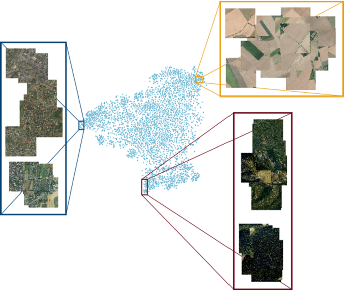

  

  2D representation of images by t-SNE after ResNet34 encoding. Similar projections are close, while different visual features are separated. In  , mostly urban scenes; in  fields images and in  mostly forest scenes

• Each point in the 2D space can be traced back to the original tile and so to the city it comes from. Then, we use a one-class SVM (Schölkopf et al. 2001) to estimate the distribution of the city images in the 2D space. It results in appearance maps which are shown in Fig. 5.

  Fig. 5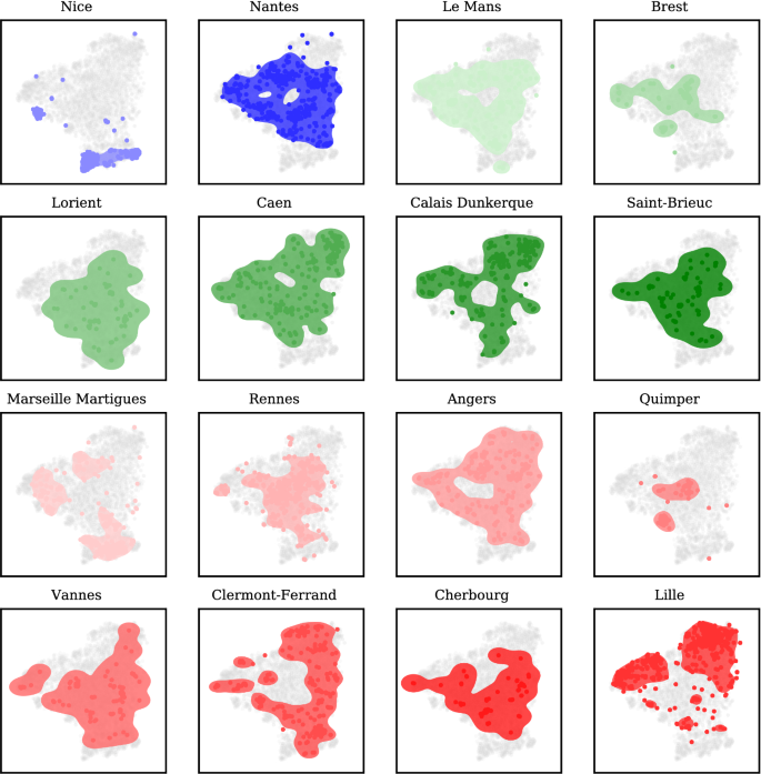

  

  Distributions of cities in the 2D appearance space

• Finally, we evaluate the appearance similarity and coverage between cities using two metrics:

  • 1. We use the intersection over union score (IoU, the standard metric for object detection) between the surfaces defined by the distributions, or appearance maps, to assess appearance similarity. Let $S_1$ and $S_2$ be two sets, the IoU score between them is defined as $IoU(S_1, S_2) = \tfrac{|S_1 \cap S_2|}{|S_1 \cup S_2|}$. In our context, higher IoU scores relate to resemblance between the appearance maps of cities.

  • 2. We also introduce the Intersection over Test area score (IoT). Let $S_1$ and $S_2$ be two sets, the IoT score between them is defined as $IoT(S_1, S_2) = \tfrac{|S_1 \cap S_2|}{|S_2|}$. This score measures the area covered by the intersection of the two surfaces normalized over the second area, which is the objective. We compute IoT considering $S_1 \in T$ and $S_2 \in E$, where T and E are the set of training cities and the set of testing cities, respectively. Thereby IoT measures how well the objective appearance map is covered by appearances of the training data.

Figure 6 shows these scores as two heatmaps between cities in the training set and the ones in the test set. Results are consistent with reality, to name a few examples: Nice exhibits low similarity scores with all cities, except Marseille, because those are the only cities from Mediterranean coast. Quimper has its higher IoU score with Brest, which is coherent because of their geographic proximity; in terms of IoT Quimper is well covered by Lorient and Saint-Brieuc, which are also geographically close (all these cities are located in Brittany). High IoU score between Angers and Caen is justified by the fact that both are agricultural localities, with similar landscapes.

Fig. 6

IoU and IoT (Intersection over Test) scores between the 2D distributions of cities in the training split and the testing split, represented as heatmaps. Last column represents the scores between a training city and the union of surfaces of the testing split. Similarly, last row corresponds to the scores between the union of surfaces in the training split and every city in the test. The dark last row of the IoT score indicates that the train split covers well every city in the test partition

To summarize, we propose a method to assess representativeness in terms of appearance similarity between cities in the MiniFrance training split and the ones in the testing split. IoU scores show that, even if there are similarities between cities, no locality in the training set is identical to another one in the test set. However, IoT proves that testing cities are well covered by the ensemble of training cities, which is confirmed by the last dark row of this score in Fig. 6 (right).

4.2 Class representativeness analysis

A class cannot be learnt if no example of it has been seen at training time. In other words, the labeled training partition has to contain all the existing classes on the dataset. If possible, the distribution of the classes during training should be similar to the one of test data.

To fulfill this condition, we study the classes distribution on the dataset. We compute class histograms of each geographic area and present them in Fig. 7. We observe that they vary significantly from one city to another. Besides, among the 12 classes that we consider in this analysis—we do not consider complex and mixed cultivation patterns, orchards at the fringe of urban classes nor clouds and shadows,⁶ see Table 3—, no city contains all of them. The best coverage of classes is given by the Nantes, Saint-Nazaire or Marseille, Martigues conurbations that exhibit 10 of the classes. However, most of the regions contain only 7 or 8 categories in total.

Fig. 7

Histograms of class distributions by city. x axis represents the classes with colors as in Table 3. y axis presents the percentage of each class by city (Color figure online)

Another problem is the heterogeneous proportions of classes in each region. The most striking example is Cherbourg where 6 classes are represented and one of them—pastures—covers 70% of the total pixels, while the other categories count for less than 10% each.

Therefore, defining a labeled training split that represents all the classes in a good proportion is not straightforward.

Along with the histograms, we make use of our precedent analysis to understand the distribution of the classes in the images in terms of appearance. Each subplot in Fig. 8 presents a class in the dataset and contains all the images in the 2D appearance representation space. Each point is colored according to the proportion occupied by the class over the image. That is, the darker the point in the figure  , the more pixels corresponding to the class are in the image. On the contrary, a light point  indicates that there are very few pixels representing the class. We observe that some classes (such as pastures or arable land) are well-spread over the whole appearance space, with high proportions in many tiles. This means that they are represented by diverse images and that they are likely to have a lot of examples (as confirmed by the histograms of Fig. 7). These classes should be easier to learn. Others—like urban fabric or industrial, commercial, public, military, private and transport units—are widespread, but do not reach majority in most of the images in which they are present. This means that these classes have a large variance in their appearance but not so many examples per appearance mode, which could make them more difficult to learn. Moreover, other categories (like artificial non-agricultural vegetated areas or herbaceous vegetation associations) are mostly concentrated over one zone—that could correspond to only one geographic region—, that is, they are present in images of specific appearances, which makes them even harder to learn. Finally, we see classes that are extremely rare (e.g. wetlands and open spaces with little or no vegetation), they are present in a few images only, and thus they should be the more difficult to learn.

Fig. 8

Class distributions in the 2D appearance space. One subplot represents one class. Each point is colored as the proportion occupied by a given class over the corresponding image (Color figure online)

All of the above shows that we can combine class distribution and visual appearance mapping to get further insight on the data. These tools help us to define a suitable partition of the MiniFrance dataset—labeled, unlabeled and test data—that satisfies the class distribution and appearance conditions as we will show in Sect. 6.2.

5 Semi-supervised semantic segmentation with deep neural networks

In this section, we introduce multi-task deep neural networks for semi-supervised semantic segmentation which will serve as baselines on the MiniFrance dataset. We aim to use unlabeled data to help generalization for semantic segmentation of aerial images. The challenge is twofold: designing network architectures able to deal with both labeled and unlabeled images, and selecting unsupervised tasks to perform along with the appropriate auxiliary loss function.

Let $\phi _s(\cdot )$ be the function learned by a supervised segmentation network (for the sake of simplicity, the corresponding network will also be referred as $\phi _s$). Such a network can be optimized through supervised learning using stochastic gradient descent and a classification loss ${\mathcal {L}}_s$ (cross entropy loss is a standard choice). We denote x the input image and y the target label, then:

$$\begin{aligned} (x,y) \mapsto {\mathcal {L}}_s( \phi _s(x), y ). \end{aligned}$$

(1)

From a general point of view, using unlabeled data to help the previous optimization can be seen as a second task optimized with a loss function ${\mathcal {L}}_u$ and a transfer function through the network denoted by $\phi _u$. Without labels, unsupervised losses usually rely on comparing in some way the output to the input image:

$$\begin{aligned} x \mapsto {\mathcal {L}}_u( \phi _u(x), x ). \end{aligned}$$

(2)

In order to improve the genericity of $\phi _s$, one has to relate $\phi _s$ and $\phi _u$. This is generally done by partially sharing parameters between both networks. Finally, the semi-supervised loss is a weighted sum of the losses for each individual task:

$$\begin{aligned} {\mathcal {L}}(x) = {\mathcal {L}}_s(\phi _s(x), y) + \lambda {\mathcal {L}}_u(\phi _u(x),x). \end{aligned}$$

(3)

5.1 Neural network architectures

We propose here two types of semi-supervised networks which process the multi-task optimization—semantic segmentation as the supervised task, along with an unsupervised task—either as parallel streams or as sequential objectives (Fig. 9).

Fig. 9

Proposed neural network architectures for semi-supervised learning. Shared layers are depicted in blue, supervised layers are in purple, and unsupervised layers are shown in green (Color figure online)

BerundaNet (with early and late task splitting) Standard encoder–decoder networks for semantic segmentation—such as SegNet (Badrinarayanan et al. 2017) or U-Net (Ronneberger et al. 2015)—can easily be extended for multiple task learning by adding a new head with a loss for the new, unsupervised task (Daudt et al. 2019; Carvalho et al. 2019). With such an architecture (thereafter named BerundaNet after the mythological two-headed bird), both tasks have shared parameters until the data streams are split. We distinguish two variants depending on the splitting layer. Early splitting networks have one encoder and two decoders, one for each task (Fig. 9a). On the contrary, with late-splitting task specialization occurs at the very end. It has an almost-all shared decoder with only a single separate convolutional layer for each task (Fig. 9b).

Eventually, all architectures optimize the global loss defined in Eq. (3). ${\mathcal {L}}_s$ can be any supervised loss for semantic segmentation, and in the following we consider the cross-entropy loss. ${\mathcal {L}}_u$ is an unsupervised loss. In the experiments we will consider reconstruction losses (such as ${\mathcal {L}}_1$ or ${\mathcal {L}}_2$) and unsupervised image segmentation losses that will be presented in Sect. 5.2.

W-Net (Xia et al. 2017; Chen et al. 2018) Multiple task learning can also be processed sequentially, as in W-Net (Xia et al. 2017) which combines two unsupervised objectives: segmentation and reconstruction. W-Net consists of two stacked U-Net (Ronneberger et al. 2015), hence its name. We adapt the original design to semi-supervised learning by specializing the first U-Net block on the semantic segmentation task and focusing the second one on the unsupervised objective (Fig. 9c). With respect to previous notations, in this case the network $\phi _s$ shares all parameters with $\phi _u$. At the end of the first U-Net block, a soft-max layer is included to achieve the supervised classification.

The loss function for our semi-supervised W-Net architecture is then more precisely decomposed as follows:

$$\begin{aligned} {\mathcal {L}}(x) = {\mathcal {L}}_s(\phi _s(x), y) + \lambda {\mathcal {L}}_u(\phi _u(\phi _s(x)),x) \end{aligned}$$

(4)

where x is the input image, y its corresponding ground truth, $\phi _s(\cdot )$ represents the first U-Net block and $\phi _u(\cdot )$ represents the second U-Net block. As before, ${\mathcal {L}}_s$ can be any supervised loss for semantic segmentation and ${\mathcal {L}}_u$ is an unsupervised loss.

This kind of architectures—BerundaNet and W-Net—allows us to deal with both labeled and unlabeled data during training. When a labeled example is processed the gradient is backpropagated trough the whole network, whereas if an unlabeled example is processed gradients are only backpropagated through the unsupervised part and shared parameters of the network (green and blue blocks in Fig. 9). However, the main objective is still the semantic segmentation task. Thus, even if unsupervised parts are helpful during the training process, evaluation can be performed without them, which yields in standard-size inference networks.

5.2 Unsupervised losses for image segmentation

We now present some unsupervised losses ${\mathcal {L}}_u$ which can leverage the information brought by images with no label. Two task objectives are usually considered, image reconstruction and image segmentation, leading to the following general formulation:

$$\begin{aligned} {\mathcal {L}}_u(\cdot ) = \alpha ^{(rec)} {\mathcal {L}}^{(rec)}(\cdot ) + \alpha ^{(reg)} {\mathcal {L}}^{(reg)}(\cdot ) \end{aligned}$$

(5)

where ${\mathcal {L}}^{(rec)}$ is a reconstruction loss, ${\mathcal {L}}^{(reg)}$ is a regularization loss and $\alpha ^{(rec)}, \alpha ^{(reg)}$ are balance coefficients.

In the following, we adapt some existing losses to semi-supervised semantic segmentation, and also propose a novel implementation of a relaxed K-means loss for unsupervised image segmentation.

Image reconstruction losses Image reconstruction losses can be simply defined using solely standard reconstruction losses such as the classical ${\mathcal {L}}_1$ and ${\mathcal {L}}_2$, as in Eqs. (6) and (7). They enforce the encoding power of internal representations built by the network $\phi _s$ by closing the loop from it to the original input, the image itself. This kind of self-supervision is for example used in Xia et al. (2017).

$$\begin{aligned} {\mathcal {L}}_1 (x) = \frac{1}{N}\sum _{i=1}^N |x_i - \hat{x}_i|, \end{aligned}$$

(6)

$$\begin{aligned} {\mathcal {L}}_2(x) = \frac{1}{N}\sum _{i=1}^N (x_i - \hat{x}_i)^2 \end{aligned}$$

(7)

where $x_i$ denotes the $i\text {th}$ pixel of the image, $\hat{x}_i$ its reconstructed version and N the number of pixels in the image.

Relaxed K-means We propose a new loss for unsupervised image segmentation, which combines the old intuitions behind the k-means algorithm with the expressive power of neural network’s non-linear modeling. In a standard manner, it is cast as a color image quantization problem, where the objective is to find an optimal, reduced set of K colors for encoding the image. Formally, it minimizes the reconstruction loss ${\mathcal {L}}^{(rec)}(x, x_c)$ where $x_c$ is the quantized image.

We still denote x the input image and $x_i$ its value at pixel i. k-means alternatively optimizes centroids of color clusters $c_k$ ($k \in \{1,K\}$) and membership matrices $\hat{y}^{(k)}$ of x to cluster k. It follows:

$$\begin{aligned} c_k =\frac{\sum _{i} x_i \hat{y}_i^{(k)}}{\sum _{i} \hat{y}_i^{(k)}} \end{aligned}$$

(8)

and

$$\begin{aligned} x_c = \sum _{k=1}^K c_k\cdot \hat{y}^{(k)} \end{aligned}$$

(9)

In standard k-means, memberships $\hat{y}_i^{(k)} \in \{0,1\}$ are then determined such that $|| x_i - c_k ||^2$ is minimum. Instead, we relax the hard constraint so that $\hat{y}_i^{(k)} \in [0,1]$ and estimate memberships as the output $\hat{y}=\phi (x)$ of a network which minimizes ${\mathcal {L}}^{(rec)}(x, x_c)$. In our experiments we will use:

$$\begin{aligned} {\mathcal {L}}_{km}^{(rec)}(x) = {\mathcal {L}}_1(x,x_c) \end{aligned}$$

(10)

Eventually, to compensate for the relaxation we add a regularization term which ensures memberships are peaked to a one-cluster-per-pixel distribution:

$$\begin{aligned} {\mathcal {L}}_{km}^{(reg)}(x) = \sum _{k=1}^K \sum _{i} \hat{y}_i^{(k)}\cdot (1-\hat{y}_i^{(k)}) \end{aligned}$$

(11)

The whole unsupervised loss is then in the form of Eq. (5).

Mumford–Shah loss Recent works on unsupervised image segmentation have brought the power of level set methods based on minimization of the Mumford–Shah functional (Mumford and Shah 1985) in CNNs (Kim and Ye 2019).

The unsupervised segmentation loss is then expressed as:

$$\begin{aligned} {\mathcal {L}}_{MS}(x) = \sum _{k=1}^K \sum _{i} |x_i - c_k|^2 \hat{y}_i^{(k)} + \alpha ^{(reg)} \sum _{k=1}^K \sum _{i} |\nabla \hat{y}_i^{(k)}| \end{aligned}$$

(12)

where we kept the same notations as before.

In Eq. (12), the first term corresponds to the reconstruction loss, while the regularization term penalizes gradient variations in the resulting segmentation, thus leading to more homogeneous regions.

6 Experiments with MiniFrance and analysis

This section intends to evaluate two aspects of our work: first, the contributions of the MiniFrance dataset with respect to existing EO datasets, and secondly, the potential of semi-supervised learning on a realistic scenario.

Furthermore, the experiments and results presented in the following will serve as baselines for future works on semi-supervised learning on the MiniFrance suite.

Implementation details For all the following experiments, networks are trained using Adam optimizer (Kingma and Ba 2015) with learning rate of $10^{-4}$, during 150 pseudo-epochs, where we observed convergence of models. Each pseudo-epoch consists of 5000 annotated samples and, in the case of semi-supervised methods, 5000 additional unlabeled samples. One sample is a 512 $\times$ 512 tile randomly chosen from training data, this patch size allows to observe enough context on one image to identify the important elements on it. In terms of losses hyperparameters for semi-supervised methods, $\lambda$ in Eq. (3) is set to $\lambda = 2.0$ for reconstruction losses (${\mathcal {L}}_1$ and ${\mathcal {L}}_2$) and to $\lambda = 5.0$ for unsupervised segmentation losses (${\mathcal {L}}_{km}$ and ${\mathcal {L}}_{MS}$) to get comparable values with respect to cross-entropy. $\alpha ^{(rec)}$ and $\alpha ^{(reg)}$ in Eq. (5) are set to $\alpha ^{(rec)} = \alpha ^{(reg)} = 1$, for simplicity. SegNet and U-Net encoders and decoders are implemented using the architectures defined on the original papers (the last layer of the decoder being adapted to the reconstruction or unsupervised segmentation loss under consideration).

PyTorch (Paszke et al. 2019) is used for all implementations. Experiments over the tinyMiniFrance dataset are executed using a Nvidia GeForce RTX 2080, while experiments over MiniFrance run on a Nvidia Tesla V100 32GB.

6.1 Limits of supervised and semi-supervised learning on standard EO datasets

The ISPRS Vaihingen dataset is a very popular dataset for semantic segmentation in EO data. It has served to benchmark several methods over the years. However, as we mentioned in Sect. 2.2, it is constrained to urban scenes over one city only and thus lacks variety.

The following results show the limits of a dataset such as Vaihingen, and prove the necessity of a more realistic dataset—that includes various locations and scenes—as offered by MiniFrance.

In our first experiment, we aim to test the sensitivity of a classic supervised learning framework to the amount of available training data. We train a SegNet model, which has already shown remarkable results on this dataset (Audebert et al. 2018). The experiment consists in reducing the amount of annotated images used for training, from 12 tiles to only one, while the validation set remains unchanged (4 tiles). We repeat the experiment four times to get more statistically significant curves. Results are shown in Fig. 10.

Fig. 10

Influence of the training set size (number of tiles) on the network performances, in terms of overall accuracy and mean Intersection over union (mIoU). The curves show the mean and the standard deviation for each score and $\star$ shows raw results

The outcomes of this experiment are somehow surprising. When reducing the number of training tiles from 12 to 1 (only 8% of original data!), we report a decrease of only 12% of overall accuracy (from 90 to 78%) and 21% of mIoU (from 77 to 56%), i.e. much less than one would expect. Indeed, we supposed that reducing the number of training tiles would seriously impact the performance of the network. One possible reason is that all the images in the Vaihingen dataset are alike, thus, to generalize on them is a relatively easy task. However, one can note that training with more data is nevertheless preferable in terms of reliability: the variance increases as the number of tiles decreases.

To investigate this explanation, we apply our tool for appearance coverage assessment presented in Sect. 4 to the union of both datasets, tinyMiniFrance and Vaihingen. To get a fair comparison, images from the Vaihingen dataset were downsampled to the tinyMiniFrance resolution (from 9 to 50 cm/px) before being encoded by the CNN.

Due to the stochastic nature of the t-SNE algorithm, it is important to note that subsequent runs can lead to different embeddings. However since tinyMiniFrance is much larger than the 16 Vaihingen tiles, the projection is not noticeably perturbed up to rotation and reflection. We chose the embedding which resulted in the same visualization as Sect. 4. Results are shown in Fig. 11. Red stars ( ) represent Vaihingen tiles, while shading blue circles ( ) are tinyMiniFrance tiles, colored according to the proportion occupied by urban fabric (as in Fig. 8, darker points contain a higher proportion of urban pixels). We consider specifically the urban fabric class since it is the most related to the Vaihingen urban dataset.

Fig. 11

2D representation of images by t-SNE, applied to tinyMiniFrance and Vaihingen together, after ResNet34 encoding. Points from tinyMiniFrance are colored according to the proportion occupied by the class urban fabric (Color figure online)

The previous visualization is insightful. On the one hand, we realize how small the Vaihingen dataset is compared to tinyMiniFrance (and even more to the entire MiniFrance), in terms of number of available tiles. On the other hand, the t-SNE algorithm places Vaihingen as a very small cluster next to the urban scenes of tinyMiniFrance, which means that: (1) Vaihingen is slightly different from tinyMiniFrance (may be due to the IRRG encoding vs. RGB); (2) at the same time, it remains visually close to the urban images from tinyMiniFrance (confirming our choice to consider here the urban fabric class); and (3) the wide surface covered by tinyMiniFrance on the 2D appearance projection space w.r.t. Vaihingen shows that our dataset presents a much larger variety of appearances in terms of urban scenes; furthermore, these urban scenes form only a small part of the appearance space, thus proving the very wide diversity of tinyMiniFrance, and to a larger extent of MiniFrance.

6.2 Defining the labeled/unlabeled/test split for MiniFrance

Using all the tools and information presented in Sect. 4, MiniFrance has been carefully designed to satisfy the conditions of appearance and class representativeness. Indeed, the split proposed in Table 2 allows to represent all the classes with a proper distribution, as shown in the histograms of Fig. 12. Hence, all classes present in the test set have training examples in the labeled split.

Fig. 12

Class distributions aggregated by split as defined in Table 2

On the appearance side as shown in Fig. 13, even if labeled cities do not cover the whole appearance space of test images, the union of labeled and unlabeled does. This should ensure that all appearances are seen in a semi-supervised setup. Moreover, in terms of IoU scores of appearance shown in Fig. 6, the labeled split comprises one region with a high score (Nantes) and one with a low score (Nice) which should help to learn different appearances of classes. In addition, in the unlabeled split most of the cities have a high score with respect to the test set, so they should help to extract the implicit information from images.

Fig. 13

Appearance representation aggregated by split as defined in Table 2

Table 5 presents the IoU and IoT scores between the surfaces in Fig. 13 and confirms the information above. Thus, even if the labeled training split contains all classes of the test split, 64% of IoT means it is far from covering all the possible appearances. However, with 93% of IoT score with the test area, the unlabeled training split offers wider information about the visual features present in the MiniFrance dataset that should be exploited to achieve good quality classification and generalization.

Table 5 IoU and IoT scores between training data—labeled and unlabeled—and test data. Scores are presented in numerical form as well as color code for comparison with Fig. 6

In brief, MiniFrance is a very challenging dataset for semantic segmentation that promotes new solutions in a semi-supervised manner as some appearances can only be extracted from the unlabeled data. However, train and test adequacy was carefully controlled to avoid domain shift and such disentangle semi-supervised learning from domain adaptation and transfer learning.

6.3 Supervised and semi-supervised learning on MiniFrance

The purpose of this section is to show that we can benefit from semi-supervised learning—using unlabeled data during the learning process—to achieve better results and generalization than vanilla supervised approaches.

To this end, we perform experiments to compare a semi-supervised setting with an equivalent supervised approach, using different backbone architectures. First, we train supervised networks (SegNet and U-Net) in a classical way, using the cross-entropy loss, over the labeled training split of tinyMiniFrance. Secondly, we train a BerundaNet-late architecture (with SegNet and U-Net backbone) over tinyMiniFrance—using both, labeled and unlabeled data—, which is the equivalent semi-supervised strategy. We train BerundaNet-late with a reconstruction task (${\mathcal {L}}_1$ as auxiliary loss) and with an unsupervised segmentation task (${\mathcal {L}}_{km}$ as auxiliary loss) and show that in both cases, semi-supervised learning can improve the results obtained by the supervised network.

Results of these experiments are summarized in Table 6. The oracle corresponds to the hypothetical case where annotations are available for all training cities (i.e, we can access the ground-truth for all the images of the 8 regions in the training split) during the training phase. The oracle results might be seen as an upper bound for semi-supervised learning strategies and they are brought out here just for comparison and not as a result of this work.

Table 6 Supervised versus semi-supervised experiments over tinyMiniFrance using different backbone architectures

Along with Table 6, Fig. 14 shows segmentation maps obtained during the testing phase for the previous experiments with a SegNet backbone. We refer as undisclosed to the entries that are not publicly available but that are shown here as a reference and comparison to our results: ground-truth and oracle. At a global scale, we observe that semi-supervised methods—whether with reconstruction or with segmentation auxiliary task—present more homogeneous and finer segmentation maps than their supervised counterpart. This is noticeable in particular in clear roads and less noisy regions. Adding unlabeled data during the learning process helps to regularize and generalize better, especially in the case of MiniFrance data, where labels are often approximate. In some cases, semi-supervised methods can even beat the oracle predictions, as in the last row example where the oracle mistook a pasture section for a water section.

Fig. 14

Classification examples of different methods. Oracle refers to the hypothetical case where all ground-truths are available for training regions (8 annotated training cities). Supervised refers to the results of a network trained only on the labeled training split of tinyMiniFrance, while semi-supervised corresponds to the BerundaNet-late network trained over all available training data (labeled and unlabeled). SegNet architecture is used as backbone

Several remarks can be raised from these results:

• First, MiniFrance is challenging. The oracle shows that even if we could access all images labels (of the 8 cities in the training split) during training, we would only get 59% overall accuracy with a fully supervised approach (see Table 6, oracle column). This is far below the accuracy that can be achieved with other datasets.

• The amount of labeled data influences a lot the performance of supervised settings. Focusing on the results of the oracle and the supervised experiment (second and third columns on Table 6), we see that for a SegNet architecture going from 8 to 2 training labeled cities implies a 22% loss in accuracy and 10% less of mIoU. And even if the U-Net seems more robust to the amount of labeled data, reducing annotated data diminishes network performances notoriously. From a visual perspective, prediction quality is noticeably worse for the supervised approach with respect to the oracle (third and forth columns in Fig. 14).

• Semi-supervised strategies exhibit promising results. In both cases, whether we use a SegNet or a U-Net backbone, the benefits of semi-supervised learning are clear, regardless of the chosen auxiliary task there is a gain of accuracy and mIoU with respect to the supervised method.

• Finally, from a visual perspective, semi-supervised methods (fifth and sixth columns in Fig. 14) are superior to the supervised one (fourth column). Indeed, semi-supervised segmentation maps are more homogeneous than the supervised ones (see the second, fourth and sixth row examples). Besides, urban cartography is better delineated in the semi-supervised semantic maps and seems more appropriated with respect to the original image.

Those are encouraging results for future works on semi-supervised learning for semantic segmentation.

6.4 Analysis of semi-supervised learning on tinyMiniFrance

We have seen that semi-supervised learning can be beneficial to improve segmentation results. Next sections intend to explore some possibilities to approach semi-supervised learning, in terms of neural network architectures or losses to use in a multi-task learning strategy.

For this purpose, we present several experiments performed over tinyMiniFrance to analyze the contributions of the neural network architectures in Sect. 6.4.1. We also study the effect of the choice of auxiliary task to perform and the unsupervised loss function in Sect. 6.4.2.

6.4.1 Influence of the choice of architecture on semi-supervision

In the following, we compare the architectures presented in Sect. 5.1 with respect to both auxiliary tasks, reconstruction (using ${\mathcal {L}}_1$ loss) and unsupervised segmentation (with ${\mathcal {L}}_{km}$ loss). For the BerundaNet-early architecture a SegNet backbone is used. Results of these experiments are reported in Table 7.

Table 7 Neural networks for semi-supervised semantic segmentation comparison

Whatever the chosen auxiliary task, BerundaNet-late with U-Net backbone is the architecture that achieves the best scores, followed by W-Net and BerundaNet-late with SegNet backbone. BerundaNet-early is just slightly better than a supervised approach with same backbone. This indicates that, in terms of network architecture, it might be better to split the supervised and unsupervised tasks rather late, enabling more shared parameters. Thus, the image statistics learned through optimization of the auxiliary task are better harnessed for the main objective.

Figures 15 and 16 show some examples of semantic maps and unsupervised outputs at inference time for these methods, using reconstruction and unsupervised segmentation as auxiliary task, respectively. From these examples, we confirm that whether we choose reconstruction or segmentation as auxiliary unsupervised task, BerundaNet-late (U-Net backbone) gets the finer and smoother results, especially in the second case.

Fig. 15

Results comparison for different neural network architectures with reconstruction as auxiliary task (${\mathcal {L}}_1$ auxiliary loss). BN-e stands for BerundaNet-early, BN-l-S/BN-l-U for BerundaNet-late with SegNet/U-Net backbone, respectively

Fig. 16

Results comparison for different neural networks with unsupervised segmentation as auxiliary task (${\mathcal {L}}_{km}$ auxiliary loss). BN-e stands for BerundaNet-early, BN-l-S/BN-l-U for BerundaNet-late with SegNet/U-Net backbone, respectively

Therefore, the choice of the architecture and backbone matters for the semi-supervised task. BerundaNet-late performs better than BerundaNet-early with same backbone. Moreover, the U-Net backbone outperforms the SegNet backbone. Finally, the simple architecture BerundaNet-late presented in this work places it first, before W-Net.

Thus, it seems the choice of architecture is at least as important as the loss design. This choice does not only rely on the number of parameters (W-Net has about twice the number of parameters of BerundaNet, since it relies on two U-Nets) but also how the supervised and unsupervised information are mixed.

6.4.2 Influence of the choice of auxiliary loss on semi-supervision

In this section, we analyze the effect on the semantic segmentation results of different auxiliary losses presented in Sect. 5.2. To this end, we train the same network architecture while changing the loss. We choose BerundaNet-late with U-Net backbone, since it was the network with the best scores in the previous sections, regardless of the auxiliary task.

Table 8 reports the results obtained through these experiments. Figure 17 exhibits some examples of segmentation maps and unsupervised outputs obtained by BerundaNet-late with reconstructions losses (${\mathcal {L}}_1$ and ${\mathcal {L}}_2$) at inference time, while Fig. 18 shows examples using unsupervised segmentation as auxiliary task.

Table 8 Auxiliary unsupervised loss effect comparison using BerundaNet-late with U-Net backbone

Fig. 17

Segmentation maps and reconstruction outputs for BerundaNet-late (U-Net backbone), using different unsupervised reconstruction losses for the auxiliary task

For the reconstruction task, ${\mathcal {L}}_1$ loss outperforms the ${\mathcal {L}}_2$ approach, this is confirmed by visual examples in Fig. 17 where we perceive that results are marginally better for ${\mathcal {L}}_1$ than for ${\mathcal {L}}_2$ in terms of smoothness, especially in urban areas like the third and fourth row examples.

In the case of segmentation, ${\mathcal {L}}_{km}$ and ${\mathcal {L}}_{MS}$ are somehow equivalent. However, from Fig. 18 the ${\mathcal {L}}_{km}$ loss seems to be superior to ${\mathcal {L}}_{MS}$ in most cases, especially when it comes to road detection.

Fig. 18

Semantic segmentation maps and unsupervised segmentation outputs for BerundaNet-late (U-Net backbone), using different unsupervised segmentation losses for auxiliary task

6.5 Experiments on the Christchurch Aerial Semantic Dataset

We also perform experiments on the Christchurch Aerial Semantic Dataset (CASD)⁷ to test the reliability of our framework (Castillo-Navarro et al. 2020).

CASD comprises aerial imagery at 10 cm/px resolution over Christchurch, New Zealand. Dense semantic annotations were produced by ONERA/DTIS on 4 images, considering 4 classes: buildings, cars, vegetation and background (Audebert et al. 2017; Randrianarivo et al. 2013). The dataset also includes 20 aerial images without annotations, which makes it suitable for semi-supervised learning algorithms.

For these experiments, we use a training partition containing labeled and unlabeled data—2 annotated tiles and 20 non-annotated tiles—, and keep 2 annotated tiles for validation. We train a BerundaNet-late architecture with U-Net backbone, because of its simplicity and efficiency. The network is trained during 50 pseudo-epochs with 5000 labeled iterations and 5000 unlabeled iterations. Since the dataset allows it (training only takes a few hours), we also evaluate different values of the hyperparameter $\lambda$ [in Eq. (3)].

Results are reported in Table 9. Mean and variance are obtained over 4 runs of each experiment. We note that semi-supervised methods outperform the supervised setting. Moreover, best scores are obtained with unsupervised segmentation losses, and especially our relaxed K-means loss allows to improve the mIoU score by + 3.39% and overall accuracy by + 1.97%, with respect to the supervised setting.

Table 9 Results comparison for supervised and semi-supervised methods over the Christchurch Aerial Semantic Dataset

Figure 19 shows two examples of segmentation maps obtained by the different methods. In the first row example, the supervised approach is the only one that mistakes the river as a building; the supplementary information provided by unlabeled images to the semi-supervised methods allows to prevent this error. In the second row, the ${\mathcal {L}}_{km}$ loss is the only one that correctly segments the central building, likely due to its color clustering capacity.

Fig. 19

Two examples of inference over the CASD dataset. buildings, cars, vegetation and background

In general, we observe from the experiments over CASD that including unlabeled data during training helps to improve the segmentation maps with respect to the case where we only use our limited labeled data.

6.6 Experiments on MiniFrance

All the results and analysis exposed above were conducted using the tinyMiniFrance dataset, due to computing capacity and processing time. In this section we present the first semi-supervised results over the entire MiniFrance dataset.

To this end, we train a BerundaNet-late with U-Net backbone as it is the best result we got in a semi-supervised setting (see Table 6). We use our regularized k-means loss (${\mathcal {L}}_{km}$) as auxiliary unsupervised loss. We also train a U-Net network on the labeled partition of MiniFrance in a classic supervised way for comparison with the semi-supervised setting. Results are reported in Table 10 and some visual results of the semi-supervised experiment are shown in Fig. 20.

Table 10 First semi-supervised results over MiniFrance

Fig. 20

Semi-supervised results over MiniFrance. BerundaNet-late with U-Net backbone and ${\mathcal {L}}_{km}$ as auxiliary loss

These results on MiniFrance are coherent with previous ones reported with tinyMiniFrance. They confirm our hypothesis that tinyMiniFrance is a good representation of the entire MiniFrance dataset. Moreover, they confirm that including unlabeled data during the learning process helps to improve the results on semantic segmentation.

It is worth to mention that training these models over the entire MiniFrance dataset for 450 pseudo-epochs takes roughly 3 weeks. While inference time—processing all the tiles on the testing partition—takes about 6 days (with a single GPU).

7 Conclusions

We have introduced the MiniFrance suite, a new large-scale dataset designed for semi-supervised semantic segmentation in Earth Observation. MiniFrance has unprecedented properties, the diversity of landscapes and scenes reflects the complexity of reality. Above all, it was thoroughly designed for semi-supervised learning, including labeled and unlabeled data in its training partition and recreating a life-like application setting, which makes MiniFrance unique. In addition to the dataset, we presented a comprehensive analysis of the data in terms of appearance similarity and representativeness, showing that MiniFrance is well-suited to address the semi-supervised problem.

We also introduced deep neural networks, based on multi-task learning, to perform semi-supervised semantic segmentation. In particular, we presented BerundaNet—a simple extension of classic encoder–decoder architectures—which proves to be very effective in the semi-supervised task. Together with these architectures, we explored unsupervised auxiliary losses to use alongside with semantic segmentation. Especially, we introduced the relaxed k-means loss to perform unsupervised image segmentation.

Our experiments have shown that we can benefit from unlabeled data during the learning process to improve semantic segmentation maps. Indeed, semi-supervised approaches allow to generate finer and more homogeneous predictions. We also observed that a simple architecture like BerundaNet-late with a suitable backbone such as U-Net is enough to enhance the segmentation performances. These results are very encouraging and will serve as baselines for future works on semi-supervised semantic segmentation over the MiniFrance dataset.

Nevertheless, the problem of semi-supervised learning is not solved. We have seen that our approaches can improve semantic segmentation results, but it is not always the case. In a multi-task approach as ours, we must be careful on the choice of architecture and the auxiliary task to perform along. Furthermore, there exist other possible ways to solve the semi-supervised problem. For instance, one could develop generative models to learn the intrinsic distribution of data from labeled and unlabeled examples and use this information together with labels to improve the segmentation. Another possibility is the use of pseudo-label methods that propagate labels from annotated examples through non-annotated ones, based on a confidence criterion, to enlarge available training data. These methods were not explored in this work, but they should be considered in future research.

References

Audebert, N., Le Saux, B., & Lefèvre, S. (2017). Segment-before-detect: Vehicle detection and classification through semantic segmentation of aerial images. Remote Sensing, 9(4), 368.
Audebert, N., Le Saux, B., & Lefevre, S. (2018). Beyond RGB: Very high resolution urban remote sensing with multimodal deep networks. ISPRS Journal of Photogrammetry and Remote Sensing, 140, 20–32.
Badrinarayanan, V., Kendall, A., & Cipolla, R. (2017). SegNet: A deep convolutional encoder–decoder architecture for image segmentation. IEEE Transactions on Pattern Analysis and Machine Intelligence, 39(12), 2481–2495. https://doi.org/10.1109/TPAMI.2016.2644615.
Bonafilia, D., Gill, J., Basu, S. & Yang, D. (2019). Building high resolution maps for humanitarian aid and development with weakly-and semi-supervised learning. In Proceedings of the IEEE conference on computer vision and pattern recognition workshops (CVPRW) (pp. 1–9).
Campos-Taberner, M., Romero-Soriano, A., Gatta, C., Camps-Valls, G., Lagrange, A., Le Saux, B., et al. (2016). Processing of extremely high-resolution LiDAR and RGB data: Outcome of the 2015 IEEE GRSS data fusion contest-part A: 2-D contest. IEEE Journal of Selected Topics in Applied Earth Observations and Remote Sensing, 9(12), 5547–5559. https://doi.org/10.1109/JSTARS.2016.2569162.
Carvalho, M., Le Saux, B., Trouvé-Peloux, P., Champagnat, F., & Almansa, A. (2019). Multi-task learning of height and semantics from aerial images. IEEE Geoscience and Remote Sensing Letters, 17(8), 1391–1395. https://doi.org/10.1109/LGRS.2019.2947783.
Castillo-Navarro, J., Audebert, N., Boulch, A., Le Saux, B., & Lefèvre, S. (2019). What data are needed for semantic segmentation in earth observation? In 2019 Joint Urban Remote Sensing Event (JURSE) (pp. 1–4). IEEE.
Castillo-Navarro, J., Le Saux, B., Boulch, A., & Lefèvre, S. (2020). On auxiliary losses for semi-supervised semantic segmentation. In European conference on machine learning and principles and practice of knowledge discovery workshops—MACLEAN (ECML-PKDD W).
Chapelle, O., Schölkopf, B., & Zien, A. (2006). Semi-supervised learning. Cambridge: The MIT Press.
Chen, L. C., Papandreou, G., Kokkinos, I., Murphy, K., & Yuille, A. L. (2017). DeepLab: Semantic image segmentation with deep convolutional nets, atrous convolution, and fully connected CRFs. IEEE Transactions on Pattern Analysis and Machine Intelligence, 40(4), 834–848.
Chen, W., Zhang, Y., He, J., Qiao, Y., Chen, Y., Shi, H., & Tang, X. (2018). W-Net: Bridged U-net for 2D medical image segmentation. arXiv preprint arXiv:1807.04459.
Chen, Z., Zhang, R., Zhang, G., Ma, Z., & Lei, T. (2020). Digging into pseudo label: A low-budget approach for semi-supervised semantic segmentation. IEEE Access, 8, 41830–41837.
Cordts, M., Omran, M., Ramos, S., Rehfeld, T., Enzweiler, M., Benenson, R., et al. (2016). The cityscapes dataset for semantic urban scene understanding. In Proceedings of the IEEE conference on computer vision and pattern recognition (CVPR) (pp. 3213–3223).
Daudt, R., Le Saux, B., Boulch, A., & Gousseau, Y. (2019). Multitask Learning For Large-Scale Semantic Change Detection. Computer Vision and Image Understanding, 187, 102783.
Demir, I., Koperski, K., Lindenbaum, D., Pang, G., Huang, J., Basu, S., et al. (2018). DeepGlobe 2018: A challenge to parse the earth through satellite images. In Proceedings of the IEEE conference on computer vision and pattern recognition workshops (CVPRW).
Demuzere, M., Bechtel, B., Middel, A., & Mills, G. (2019). Mapping Europe into local climate zones. PLOS ONE, 14(4), 1–27. https://doi.org/10.1371/journal.pone.0214474.
Deng, J., Dong, W., Socher, R., Li, L. J., Li, K., & Fei-Fei, L. (2009). ImageNet: A large-scale hierarchical image database. In Proceedings of IEEE conference on computer vision and pattern recognition (CVPR) (pp. 248-255).
Durand, T., Mordan, T., Thome, N., & Cord, M. (2017). WILDCAT: Weakly supervised learning of deep ConvNets for image classification, pointwise localization and segmentation. In IEEE conference on computer vision and pattern recognition (CVPR) (Vol. 2).
Fisher, P., Comber, A. J., & Wadsworth, R. (2005). Land use and land cover: Contradiction or complement. Re-presenting GIS (pp. 85–98).
Gupta, R., Goodman, B., Patel, N., Hosfelt, R., Sajeev, S., Heim, E., et al. (2019). Creating xBD: A dataset for assessing building damage from satellite imagery. In Proceedings of the IEEE conference on computer vision and pattern recognition workshop computer vision for global challenges (CVPRW).
Haala, N., Cramer, M., & Jacobsen, K. H. (2010). The German Camera Evaluation Project—results from the geometry group. In Canadian geomatics conference and symposium of commission I—geometry. https://doi.org/10.15488/1119.
He, K., Zhang, X., Ren, S., & Sun, J. (2016). Deep residual learning for image recognition. In Proceedings of the IEEE conference on computer vision and pattern recognition (CVPR) (pp. 770–778).
Hong, D., Yokoya, N., Ge, N., Chanussot, J., & Zhu, X. X. (2019). Learnable manifold alignment (LeMA): A semi-supervised cross-modality learning framework for land cover and land use classification. ISPRS Journal of Photogrammetry and Remote Sensing, 147, 193–205.
Hung, W. C., Tsai, Y. H., Liou, Y. T., Lin, Y. Y., & Yang, M. H. (2018). Adversarial learning for semi-supervised semantic segmentation. In Proceedings of the British machine vision conference (BMVC).
Kalluri, T., Varma, G., Chandraker, M., & Jawahar, C. (2019). Universal semi-supervised semantic segmentation. In Proceedings of the IEEE international conference on computer vision (ICCV) (pp. 5259–5270).
Khoreva, A., Benenson, R., Hosang, J. H., Hein, M., & Schiele, B. (2017). Simple does it: Weakly supervised instance and semantic segmentation. In Proceedings of the IEEE conference on computer vision and pattern recognition (CVPR).
Kim, B., & Ye, J. C. (2019). Mumford–Shah loss functional for image segmentation with deep learning. IEEE Transactions on Image Processing.
Kingma, D. P., & Ba, J. (2015). Adam: A method for stochastic optimization. In Proceedings of the international conference on learning representations (ICLR).
Lam, D., Kuzma, R., McGee, K., Dooley, S., Laielli, M., Klaric, M., Bulatov, Y., & McCord, B. (2018). xView: Objects in context in overhead imagery. arXiv e-prints
Le, H., Gonçalves, B., Samaras, D., & Lynch, H. (2019). Weakly labeling the Antarctic: The Penguin Colony case. In Proceedings of the IEEE conference on computer vision and pattern recognition workshops (CVPRW) (pp. 18–25).
Lee, D. H. (2013). Pseudo-label: The simple and efficient semi-supervised learning method for deep neural networks. In Proceedings of the international conference on machine learning workshop on challenges in representation learning (ICMLW) (Vol. 3, p. 2).
Lefebvre, A., Sannier, C., & Corpetti, T. (2016). Monitoring urban areas with sentinel-2A data: Application to the update of the Copernicus high resolution layer imperviousness degree. Remote Sensing, 8(7), 606.
Lin, T. Y., Maire, M., Belongie, S., Hays, J., Perona, P., Ramanan, D., et al. (2014). Microsoft COCO: Common objects in context. In Proceedings of European conference on computer vision (ECCV) (pp. 740–755). Berlin: Springer.
Long, J., Shelhamer, E., & Darrell, T. (2015). Fully convolutional networks for semantic segmentation. In Proceedings of the IEEE conference on computer vision and pattern recognition (CVPR) (pp. 3431–3440).
Maaten, L. V. D., & Hinton, G. (2008). Visualizing data using t-SNE. Journal of Machine Learning Research, 9, 2579–2605.
Maggiolo, L., Marcos, D., Moser, G., & Tuia, D. (2018). Improving maps from CNNs trained with sparse, scribbled ground truths using fully connected CRFs. In Proceedings of the IEEE international symposium on geoscience and remote sensing (IGARSS).
Maggiori, E., Tarabalka, Y., Charpiat, G., & Alliez, P. (2017). Can semantic labeling methods generalize to any city? The INRIA aerial image labeling benchmark. In Proceedings of the IEEE international symposium on geoscience and remote sensing (IGARSS). https://doi.org/10.1109/IGARSS.2017.8127684.
Minaee, S., Boykov, Y., Porikli, F., Plaza, A., Kehtarnavaz, N., & Terzopoulos, D. (2020). Image segmentation using deep learning: A survey. arXiv preprint arXiv:2001.05566.
Mnih, V., & Hinton, G. (2010). Learning to detect roads in high-resolution aerial images. In Proceedings of the European conference on computer vision (ECCV).
Montero, E., Van Wolvelaer, J., & Garzón, A. (2014). The European Urban Atlas. In Land use and land cover mapping in Europe (pp. 115–124). Springer.
Mumford, D., & Shah, J. (1985). Boundary detection by minimizing functionals. In Proceedings of the IEEE conference on computer vision and pattern recognition (CVPR), (Vol. 17, pp. 137-154).
Nivaggioli, A., & Randrianarivo, H. (2019). Weakly supervised semantic segmentation of satellite images. In 2019 Joint Urban Remote Sensing Event (JURSE) (pp. 1–4). IEEE.
Paisitkriangkrai, S., Sherrah, J., Janney, P., & Van-Den Hengel, A. (2015). Effective semantic pixel labelling with convolutional networks and conditional random fields. In Proceedings of the IEEE conference on computer vision and pattern recognition workshops (CVPRW).
Papandreou, G., Chen, L. C., Murphy, K. P., & Yuille, A. L. (2015). Weakly-and semi-supervised learning of a deep convolutional network for semantic image segmentation. In Proceedings of the IEEE international conference on computer vision (ICCV) (pp. 1742–1750).
Paszke, A., Gross, S., Massa, F., Lerer, A., Bradbury, J., Chanan, G., et al. (2019) PyTorch: an imperative style, high-performance deep learning library. In Advances in neural information processing systems 32 (NeurIPS).
Randrianarivo, H., Le Saux, B., & Ferecatu, M. (2013). Urban structure detection with deformable part-based models. In 2013 IEEE international geoscience and remote sensing symposium (IGARSS) (pp. 200–203). IEEE.
Rey, N., Volpi, M., Joost, S., & Tuia, D. (2017). Detecting animals in African Savanna with UAVs and the crowds. Remote Sensing of Environment, 200, 341–351.
Ronneberger, O., Fischer, P., & Brox, T. (2015). U-net: Convolutional networks for biomedical image segmentation. In Proceedings of the international conference on medical image computing and computer-assisted intervention (MICCAI) (pp. 234–241). Berlin: Springer.
Rottensteiner, F., Sohn, G., Gerke, M., & Wegner, J. D. (2014). Journal of Photogrammetry and Remote Sensing: Special issue on Urban object detection and 3D building reconstruction (Vol. 93). Elsevier.
Runting, R. K., Phinn, S., Xie, Z., Venter, O., & Watson, J. E. (2020). Opportunities for big data in conservation and sustainability. Nature Communications, 11(1), 1–4.
Schmitt, M., Prexl, J., Ebel, P., Liebel, L., & Zhu, X. X. (2020). Weakly supervised semantic segmentation of satellite images for land cover mapping—challenges and opportunities. arXiv preprint arXiv:2002.08254.
Schölkopf, B., Platt, J. C., Shawe-Taylor, J., Smola, A. J., & Williamson, R. C. (2001). Estimating the support of a high-dimensional distribution. Neural Computation, 13(7), 1443–1471.
Simonyan, K., & Zisserman, A. (2015). Very deep convolutional networks for large-scale image recognition. In Proceedings of the international conference on learning representations (ICLR).
Souly, N., Spampinato, C., & Shah, M. (2017). Semi-supervised semantic segmentation using generative adversarial network. In Proceedings of the IEEE international conference on computer vision (ICCV) (pp. 5688–5696).
Sumbul, G., Charfuelan, M., Demir, B., & Markl, V. (2019). Bigearthnet: A large-scale benchmark archive for remote sensing image understanding. In IEEE international geoscience and remote sensing symposium (IGARSS).
Tao, Y., Xu, M., Zhang, F., Du, B., & Zhang, L. (2017). Unsupervised-restricted deconvolutional neural network for very high resolution remote-sensing image classification. IEEE Transactions on Geoscience and Remote Sensing, 55(12), 6805–6823.
Tuia, D., Volpi, M., Trolliet, M., & Camps-Valls, G. (2014). Semisupervised manifold alignment of multimodal remote sensing images. IEEE Transactions on Geoscience and Remote Sensing, 52(12), 7708–7720.
Xia, G. S., Bai, X., Ding, J., Zhu, Z., Belongie, S., Luo, J., et al. (2018). DOTA: A large-scale dataset for object detection in aerial images. In Proceedings of the IEEE conference on computer vision and pattern recognition (CVPR) (pp. 3974–3983).
Xia, J., Chanussot, J., Du, P., & He, X. (2013). (Semi-) supervised probabilistic principal component analysis for hyperspectral remote sensing image classification. IEEE Journal of Selected Topics in Applied Earth Observations and Remote Sensing, 7(6), 2224–2236.
Xia, X., & Kulis, B. (2017). W-Net: A deep model for fully unsupervised image segmentation. arXiv e-prints arXiv:1711.08506.
Zhang, R., Albrecht, C., Zhang, W., Cui, X., Finkler, U., Kung, D., & Lu, S. (2020). Map generation from large scale incomplete and inaccurate data labels. arXiv preprint arXiv:2005.10053.
Zhao, H., Shi, J., Qi, X., Wang, X., & Jia, J. (2017) Pyramid scene parsing network. In Proceedings of the IEEE conference on computer vision and pattern recognition (CVPR) (pp. 2881–2890).
Zhu, R., Yan, L., Mo, N., & Liu, Y. (2019). Semi-supervised center-based discriminative adversarial learning for cross-domain scene-level land-cover classification of aerial images. ISPRS Journal of Photogrammetry and Remote Sensing, 155, 72–89.
Zhu, X. X., Tuia, D., Mou, L., Xia, G. S., Zhang, L., Xu, F., & Fraundorfer, F. (2017). Deep learning in remote sensing: A comprehensive review and list of resources. IEEE Geoscience and Remote Sensing Magazine, 5(4), 8–36.
Acknowledgements
Javiera Castillo-Navarro’s work is partially funded by a grant from Centre National d’Études Spatiales (CNES). The authors acknowledge the IGN for providing the BD ORTHO database under Open Licence v1.0 (https://www.etalab.gouv.fr/licence-ouverte-open-licence) and the European Copernicus Program for providing the Urban Atlas data (https://land.copernicus.eu/local/urban-atlas). This work contains modified Copernicus Urban Atlas data.
Author information
Authors and Affiliations
Corresponding author
Additional information
Publisher's Note
Springer Nature remains neutral with regard to jurisdictional claims in published maps and institutional affiliations.
Editors: Dino Ienco, Thomas Corpetti, Minh-Tan Pham, Sebastien Lefevre, Roberto Interdonato.
Rights and permissions
About this article
Cite this article
Castillo-Navarro, J., Le Saux, B., Boulch, A. et al. Semi-supervised semantic segmentation in Earth Observation: the MiniFrance suite, dataset analysis and multi-task network study. Mach Learn 111, 3125–3160 (2022). https://doi.org/10.1007/s10994-020-05943-y
Received:
Revised:
Accepted:
Published:
Issue Date:
DOI: https://doi.org/10.1007/s10994-020-05943-y