
Perturbations of the Gravitational Energy in the TEGR: Quasinormal Modes of the Schwarzschild Black Hole
by
 , , and
José Wadih Maluf
1,* ,
,
Sérgio Ulhoa
1,
Fernando Lessa Carneiro
1 and
Karlúcio H. C. Castello-Branco
2 1
Instituto de Física, Universidade de Brasília, Brasília, DF 70919-970, Brazil
2
Instituto de Ciências da Educação, Universidade Federal do Oeste do Pará, Santarém, PA 68040-070, Brazil
*
Author to whom correspondence should be addressed.
Universe 2021, 7(4), 100; https://doi.org/10.3390/universe7040100
Submission received: 1 March 2021
/
Revised: 7 April 2021
/
Accepted: 8 April 2021
/
Published: 14 April 2021
(This article belongs to the Special Issue Teleparallel Gravity: Foundations and Observational Constraints)
Abstract
:We calculate the gravitational energy spectrum of the perturbations of a Schwarzschild black hole described by quasinormal modes, in the framework of the teleparallel equivalent of general relativity (TEGR). We obtain a general formula for the gravitational energy enclosed by a large surface of constant radius r, in the region , where m is the mass of the black hole. Considering the usual asymptotic expression for the perturbed metric components, we arrive at finite values for the energy spectrum. The perturbed energy depends on the two integers n and l that describe the quasinormal modes. In this sense, the energy perturbations are discretized. We also obtain a simple expression for the decrease of the flux of gravitational radiation of the perturbations.
1. Introduction
The response of a black hole or neutron star to external, nonradial perturbations is described by quasinormal modes. A comprehensive review of the physics related to this interesting phenomena is found in [1,2]. These modes are damped oscillations of the space-time geometry that may be used to characterize the intrinsic properties of the physical system. Investigations on quasinormal modes are carried out both analytically and numerically. The modes are characterized by a spectrum of discrete, complex valued frequencies. The real part of the frequency is related to the oscillation frequency, and the imaginary part yields the rate at which each mode is damped as a result of emission of radiation. Thus, quasinormal modes may be important to gravitational waves astrophysics. In addition, the study of these modes is, to some extent, a testing ground for ideas in quantum gravity. Chandrasekhar once stated [3] that one relevant way of investigating a physical system is by perturbing it, and then analyzing the response of the system. This is precisely the role of QNM in the context of black holes.
In the analysis of Einstein’s equations for a perturbed Schwarzschild space-time, one finds a number of equations that are eventually reduced to two one-dimensional wave equations for the perturbed metric components (for axial and polar perturbations) [1]. However, the nature of the potential in these equations precludes exact solutions in terms of known functions [4]. In particular, the equations for the metric perturbations admit solutions provided the frequencies are discrete and under the imposition of special boundary conditions. The solutions of these equations are the quasinormal modes.
In this article, we calculate the energy spectrum of the quasinormal modes in the framework of the teleparallel equivalent of general relativity (TEGR). A proper definition for the energy–momentum of the gravitational field is of ultimate importance for a comprehensive understanding of Einstein’s general relativity, and yet there is no general agreement regarding an acceptable expression. There is no unique approach to the problem (e.g., pseudotensors and quasilocal expressions), and even within each approach there is no preferred definition for the energy–momentum. In the context of the field equations of the TEGR, however, one finds a suitable and consistent framework for the definitions of the gravitational energy–momentum and 4-angular momentum [5,6], which satisfy the algebra of the Poincaré group. This definition of the gravitational energy–momentum has been applied to several configurations of the gravitational field, and leads to consistent results. It satisfies important requirements that any gravitational energy–momentum definition must satisfy [6].
We consider the perturbed Schwarzschild space-time and calculate the gravitational energy enclosed by a surface of constant radius r. The energy contained within this region of the unperturbed space-time is known and may be easily evaluated out of the definition that arises in the TEGR, as well as by means of several quasilocal definitions for the gravitational energy. Thus, by subtracting the unperturbed energy from the total energy that includes the perturbations, we obtain the energy of the perturbations only. In the present analysis, we will consider both axial and polar perturbations. We restrict the analysis to gravitational perturbations (we do not address scalar and electromagnetic perturbations). We find that the perturbed energy: (i) oscillates and at the same time is damped; and (ii) depends on the integers n (the overtone number) and l (the angular momentum number). To our knowledge, a similar analysis regarding the spectrum of the energy perturbations of the Schwarzschild space-time has not been presented thus far. We conjecture that the perturbed energy in arbitrary (nonspherical) volumes of the Schwarzschild space-time is also characterized by integers.
Notation: space-time indices and SO(3,1) indices run from 0 to 3. Time and space indices are indicated according to . The tetrad field is denoted , and the torsion tensor reads . The flat, Minkowski space-time metric tensor raises and lowers tetrad indices and is fixed by . The determinant of the tetrad field is represented by .
2. Review of the Gravitational Energy–Momentum Definition in the TEGR
We assume that the space-time geometry is defined by the tetrad field only. In this case, the only possible nontrivial definition for the torsion tensor is given by . In the TEGR, it is possible to rewrite Einstein’s equations in terms of and . The Lagrangian density of the theory is defined by
where , , and
stands for the Lagrangian density for the matter fields. The Lagrangian density L is invariant under the global SO(3,1) group. Invariance under the local SO(3,1) group is verified as long as we take into account the total divergence that arises in the identity
where is the scalar Riemannian curvature. However, the field equations derived from Equation (1) are invariant under local SO(3,1) transformations and are equivalent to Einstein’s equations. They read
where .
The definition of the gravitational energy–momentum may be established in the framework of the Lagrangian formulation defined by (1), according to the procedure of ref. [5] (we make ). Equation (3) may be rewritten as
where and is defined by
In view of the antisymmetry property , it follows that
The equation above yields the continuity (or balance) equation,
Therefore, we identify as the gravitational energy–momentum tensor [5],
as the total energy–momentum contained within a volume V,
as the gravitational energy–momentum flux [7,8], and
as the energy–momentum flux of matter [8]. In view of (4), Equation (8) may be written as
where . A summary of all issues discussed above can be found in [9].
Equation (11) is the definition for the gravitational energy–momentum presented in [6], obtained in the framework of the vacuum field equations in Hamiltonian form. It is invariant under coordinate transformations of the three-dimensional space and under time reparameterizations. Note that (6) is a true energy–momentum conservation equation. We also remark that for finite volumes of integration, the free index of the integral of the energy–momentum 4-vector density must be a Lorentz index, such as a in the left hand side of definition (11), because under a global SO(3,1) transformation both sides of (11) transform consistently. In contrast, the integral on the right hand side of a hypothetical quantity such as (with space-time index ) would be coordinate dependent (the integral of a space-time vector density is neither invariant nor covariant under coordinate transformations), and therefore ill-defined for finite, three-dimensional volumes of integration.
In the ordinary formulation of arbitrary field theories, energy, momentum, angular momentum and the center of mass moment are frame dependent field quantities, which transform under the global SO(3,1) group. In particular, energy transforms as the zero component of the energy–momentum four-vector. These features of special relativity must also hold in general relativity, since the latter yields the former in the limit of weak (or vanishing) gravitational fields. As an example, consider the total energy of a black hole, represented by the mass parameter m. As seen by a distant observer, the total energy of a static Schwarzschild black hole is given by . However, at great distances, the black hole may be considered as a particle of mass m, and, if it moves with constant velocity v, then its total energy as seen by the same distant observer is , where . Likewise, the gravitational momentum, angular momentum, and the center of mass moment are naturally frame dependent field quantities, whose values vary from frame to frame and are different for different observers in arbitrary space-times.
Before closing this section, we note that the existence of a scalar density (on a three-dimensional spacelike hypersurface) such as in Equation (11) is natural in the framework of theories constructed out of third-order tensors such as the torsion tensor . Naively, we observe that the contraction of two space-time indices in a third order tensor yields a vector of the type , and therefore is a well defined scalar density that under integration yields a well behaved surface integral, in similarity to Equation (11). The existence of these well defined scalar densities is natural in the TEGR, as in the identity below Equation (2), but, of course, after a number of manipulations and rearrangements, these scalar densities could also be established in Einstein–Cartan type theories.
3. Axial Perturbations of the Schwarzschild Black Hole
The analysis of the quasinormal modes in the Schwarzschild space-time consists in solving the differential equations for the perturbed metric components, with appropriate boundary conditions. These equations were first written down by Regge and Wheeler [10]. They obtained the general form of the simplest nonspherical perturbations for the Schwarzschild black hole, namely the axial and polar perturbations. Regge and Wheeler showed that the equations that describe the axial perturbations may be separated if the perturbed metric tensor is expanded in tensorial spherical harmonics. The general form of is obtained and further simplified by taking into account the gauge symmetry (coordinate invariance) of the field equations. The simplest form of the nonvanishing axial perturbations are given by [10]
where are the Legendre polynomials. The functions and satisfy the equations [1,10]
where . Equation (15) is a consequence of (13) and (14). The quantity in (13) may be substituted in (14). Thus, (13) and (14) may be combined into one equation. Defining , the resulting equation reads
In terms of the tortoise coordinate , Equation (16) may be rewritten as
is the Regge–Wheeler potential, which is given by
and .
The time dependence of is assumed to be of the type , where is a complex frequency. Thus, it follows that . As a consequence, the function satisfies the time independent equation
In view of the asymptotic behavior of the potential , the expressions of in the asymptotic limits and are given by and , respectively, where in order to ensure the perturbative character of the solution. Expressions with positive exponential correspond to waves that are purely outgoing at infinity, and the ones with negative exponential to waves that are purely ingoing at the horizon.
For weakly excited states, the quasinormal frequencies may be obtained from the third-order WKB approximation. In the case of the gravitational perturbation, the fundamental state is given by and [11,12]. These semi-analytic approximations yield values very close to the numerical values [13]. The stable solutions decay with time. Thus, if and represent the real and imaginary parts, respectively, of the complex valued frequency, then we must have .
The possible values of for highly damped modes (large values of n) are independent of l, and may be obtained by means of numerical investigations. They are given by [1]
where n is an integer. This expression has also been obtained by means of analytic procedure in [14]. However, the frequency to be employed in the construction of the figures below, in Section 4 and Section 5, does not correspond to highly damped modes.
The problems regarding the divergent behavior of in the limit were discussed by ref. [1] (Section 4) and ref. [15]. However, the asymptotic behavior of poses no problem to the result of our analysis, since we integrate (11) over a surface of constant (finite) radius .
We need the asymptotic behavior of . Given that , and
which follows from (13) in the limit , we find
The correction to the expressions above is negligible in the development of our analysis. By means of straightforward calculations, we obtain from (22) an expression that holds in the limit and is useful in the following subsection. We find
4. The Gravitational Energy of the Axial Perturbations
In this section, we address the axially perturbed Schwarzschild space-time and calculate the gravitational energy contained within a simple three dimensional volume, namely a spherical volume of radius r. To simplify the calculations, we consider a large sphere so that the field quantities are considered in the limit . The purpose is to find the expression of the energy perturbations in this limit. To our knowledge, no expression for the gravitational energy perturbations has been obtained thus far in the present physical context.
In the course of the calculations, we find that the perturbed gravitational energy depends on the square of the field quantities and that appear in (12). Therefore, to calculate the first-order contribution to the perturbed energy, we must keep the terms quadratic in and .
We start with the metric tensor [10]
Definition (11) for the gravitational energy–momentum is frame dependent. Thus, we choose a configuration of tetrad fields that has a clear physical interpretation. Tetrad fields are interpreted as reference frames adapted to preferred fields of observers in space-time. This interpretation is possible by identifying the components of the frame with the four-velocities of the observers, [16,17]. In the present analysis, we establish a set of tetrad fields adapted to static observers in space-time. Therefore, we require . This condition fixes three components of the frame. The other three components are fixed by choosing a orientation of the frame in the three-dimensional space. Thus, is parallel to the worldline of the observers and are the three unit vectors orthogonal to the timelike direction. We fix such that , and in Cartesian coordinates are unit vectors along the x, y and z directions. The tetrad field in coordinates that satisfies these conditions is given by
with the following definitions:
The frame above satisfies . It is possible to show that if we neglect and , the frame components in the limit are given by , and .
We denote by g and e the determinants of and , respectively. We find . Thus, we have
The gravitational energy is given by the component of (11). Transforming the volume integral into a surface integral and considering the definition , we find that
The integration is carried out on a surface S of constant radius r.
The non-vanishing components of the torsion tensor that are relevant to the evaluation of the gravitational energy are
The evaluation of requires a large number of algebraic manipulations, but otherwise it is simple. The full expression of is given by
By keeping terms of order and only in the integrand of (31), we obtain the approximate expression that is relevant to the present analysis. The leading term in the energy expression is m, the total Schwarzschild energy. It is easy to verify that
which is a well known result. We recall that B is given by (27).
The gravitational energy of the perturbations is denoted by and is obtained out of the second-order terms in (31), assuming and . Therefore, for fixed values of r such that , we obtain, after some simplifications,
Recalling that (we are assuming ), we find
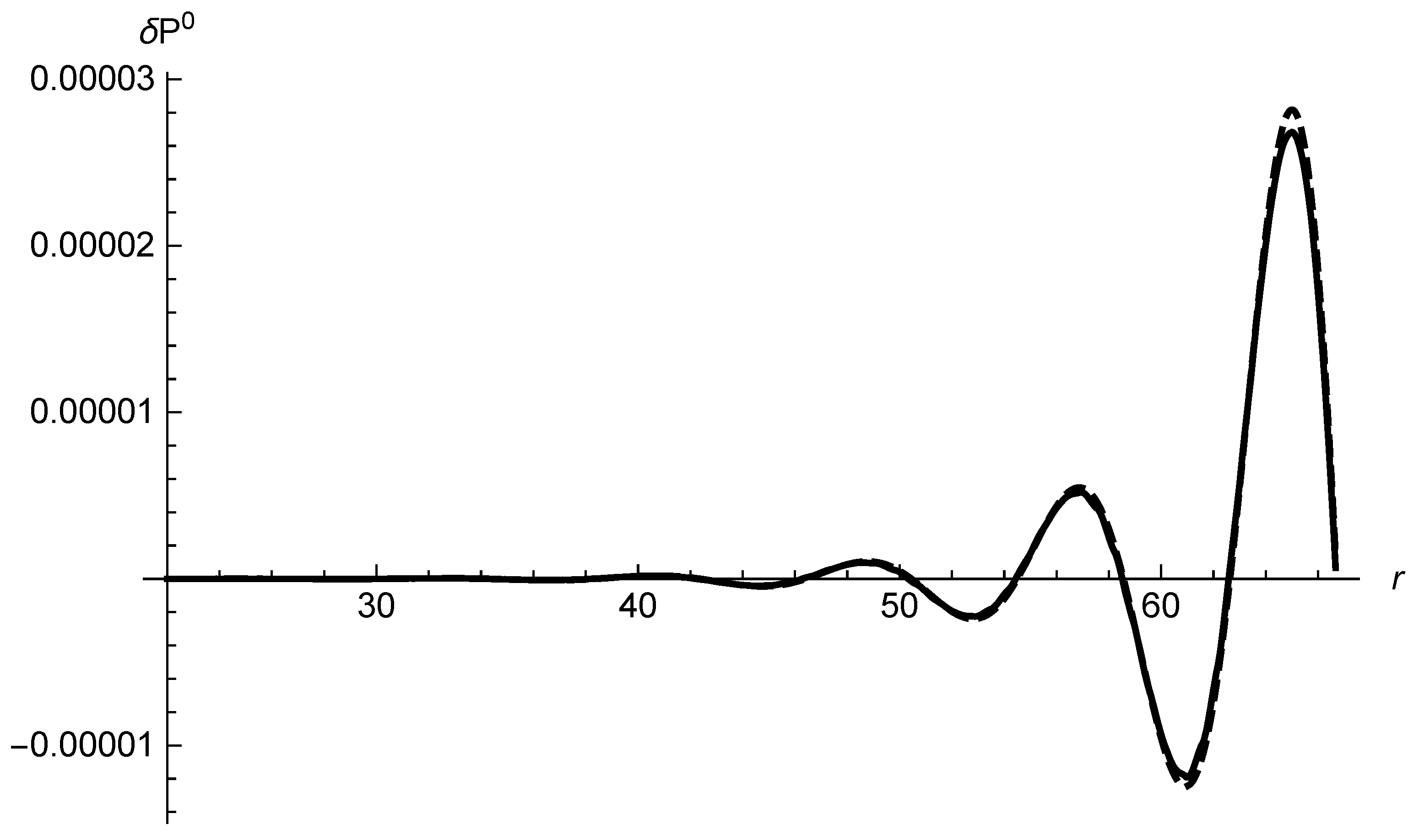
In the absence of the perturbation, i.e., when , vanishes. The approximate solution (34) may be compared with the numerical solution presented in Figure 1. The numerical solution, represented by the continuous line, is obtained directly from the exact expression for the total gravitational energy minus the black hole energy, requiring the function to be a solution of Equation (19). The boundary conditions for the numerical solution of Equation (19) are and , where , , and .
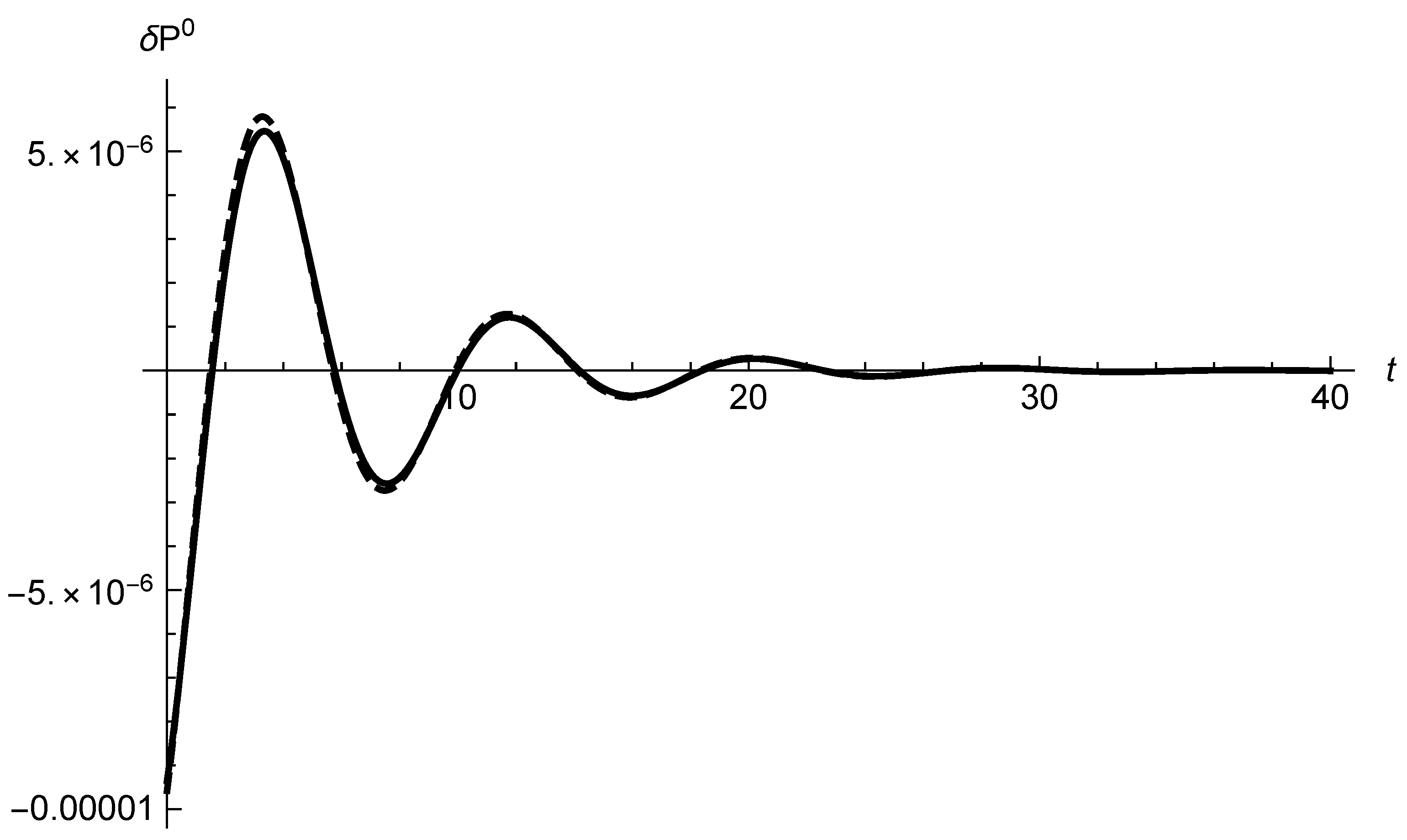
In Figure 1, we display the initial instant of time of the perturbation. We see that the larger is the value of the coordinate r, more intense is the energy of the perturbation, probably because the farther one is from the black hole, the more energy is necessary to perturb it. Note that r is not a dynamical coordinate, it is just a parameter of the coordinate system that fixes the radius of integration. The evolution of the gravitational energy perturbation is stable, i.e., the latter tends to zero when , as shown in Figure 2.
Considering the real part of the solution given by Equation (34), we have
We may calculate the variation of the perturbation energy in a half-life interval , for weakly damped solutions, but neglecting the damping effects, considering only . By making use of
we obtain
Since the black hole looses energy in the course of time, as shown in Figure 2, it is important to analyze the rate at which the energy decay occurs. This issue may be described by the energy flux of the radiated energy. The present formalism for the gravitational energy–momentum allows a definition for the gravitational energy–momentum flux [8], which is applied to the radiation of gravitational energy in the Bondi space-time. The gravitational energy flux is given by the component of defined by (9), or simply by
In the present context, we find
Again, we define and find that after the period the decrease in the flux of gravitational radiation is , and therefore
5. Polar Perturbations of the Schwarzschild Black Hole
In this section, we repeat the analysis developed in the previous section for the axial perturbations. In the context of polar perturbations, the calculations are more intricate, despite the similarities with the calculations carried out for the axial perturbations. We consider the perturbed metric tensor as given by . The line element for the unperturbed metric tensor is
and the polar perturbations are described by [10]
where and , , , and K are functions of . Therefore, the perturbed metric tensor is written as
where we define
Einstein’s equations reduce to seven non-trivial equations: one algebraic equation, three first-order differential equations for the metric tensor components, and three second-order equations. The algebraic equation is eventually reduced to [10]
The three remaining equations eventually yield the algebraic equation
where .
By rewriting the field quantities according to [18]
and
and defining the tortoise coordinate x as
we obtain the relations
It follows that
and
where
is the Zerilli potential.
Although the algebraic forms of the Zerilli and Regge–Wheeler potentials are quite distinct, they share strong similarities [1]. For very large values of the coordinate r, we have . Thus, in the limit , we obtain a simple solution for the function , given by
where A is a constant with dimension of length. To ensure the perturbative character of the solution, the amplitude A is required to satisfy , in natural units. In the limit , the solution grows with the radial distance. Thus, since the approximations are made assuming , we must ensure that . The frequencies of the polar perturbations are the same as for the axial perturbations [19], provided we consider the same values of when comparing the frequencies. Considering as usual , we have
It is important to remark that the stability of the solutions demand that the function decay sufficiently quickly with time. Consequently, the stable solutions are those for which . The solutions obtained in the following approximations are valid as long as
Therefore, the approximate analytic solutions are valid provided the condition is satisfied.
As in the axial case, we must find the asymptotic limits for the perturbative functions. Thus, in the limit , Equations (52)–(55) become
The expressions above given by Equations (65)–(67) are used in the following subsection, where we evaluate the gravitational energy of the polar perturbations.
The Gravitational Energy of the Polar Perturbations
Similar to the analysis in Section 4, where we address the gravitational energy of the axial perturbations, here we construct a set of tetrad fields adapted to static observers (with respect to the asymptotic flat space-time limit of the black hole), which yields the metric tensor (43). A set of tetrad fields that satisfy the necessary conditions is given by
where
and whose determinant is .
The components of the torsion tensor and the tensor that are needed in the calculations below are
and
With the help of these quantities, we find
The expression above leads to the gravitational energy given by Equation (11). An approximate analytic expression for the quantity above may be obtained by considering terms up to the second order in , and K. The unperturbed expression of the momentum given by Equation (72) is simply . The integration of this quantity on a surface at spacelike infinity yields the expected expression for the total gravitational energy, . Thus, the quantity that yields the gravitational energy of the perturbations is . The approximate analytic expression of the latter is
The first line in (73) contains the first order terms , whereas the other terms correspond to the second-order terms . The total energy within a spherical surface of radius r is obtained by summing these two quantities, and integrating over the spherical surface. The first-order terms depend on the variable in the form . The integration of this quantity vanishes, i.e., . Therefore, only the second-order terms yield a non-trivial result when integrated over the whole spherical shell.
Using the results given by Equations (65)–(67), we integrate (73) over a spherical surface of radius r and obtain the gravitational energy of the perturbation. We find
where . In view of the orthogonality property of the Legendre polynomials,
we obtain
Similar to the axial case, the final result given by Equation (75) has real and imaginary parts, both in the exponential and in the frequency . As before, we take the real part of the whole expression. In the case of highly damped oscillations, we have , and therefore we may use .
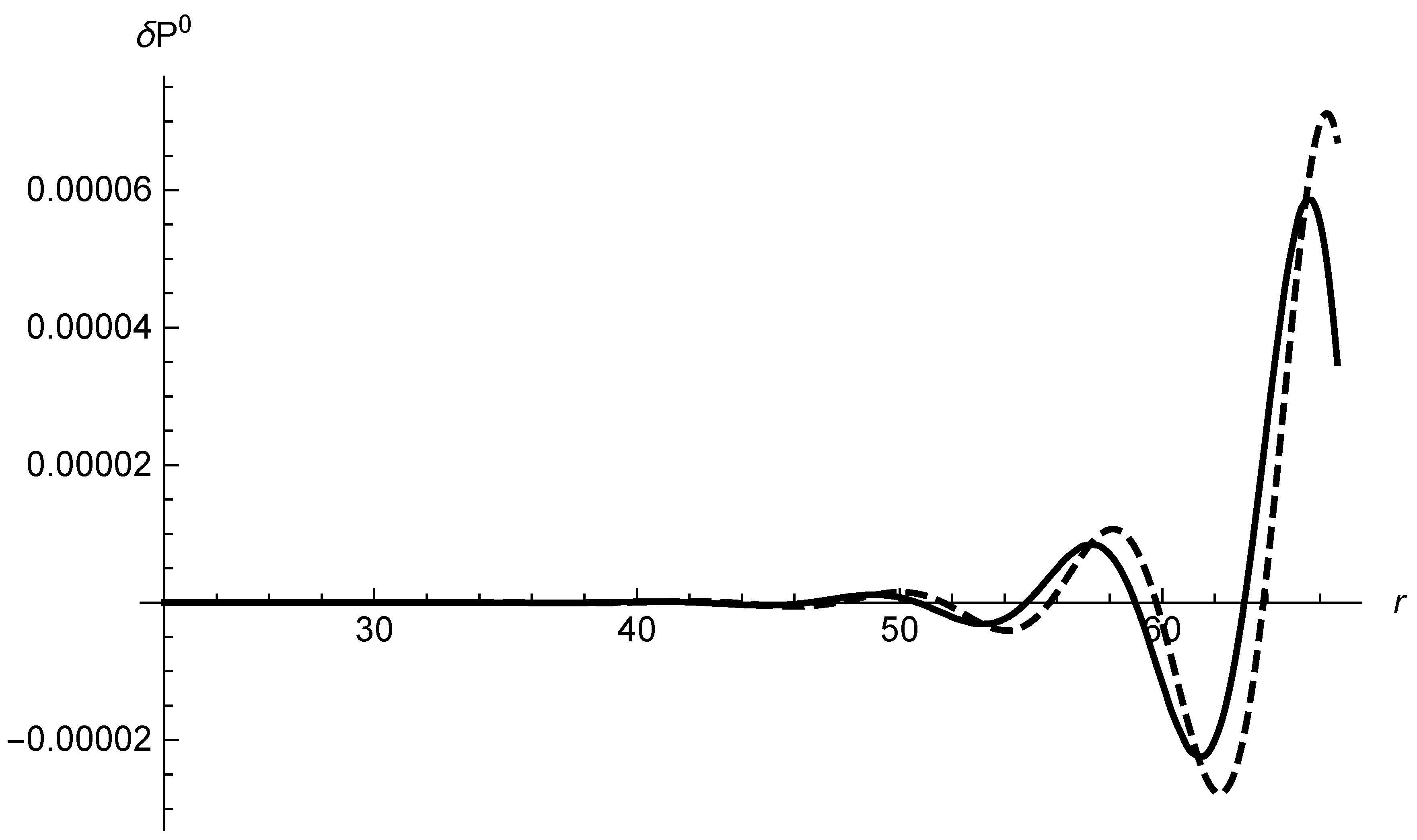
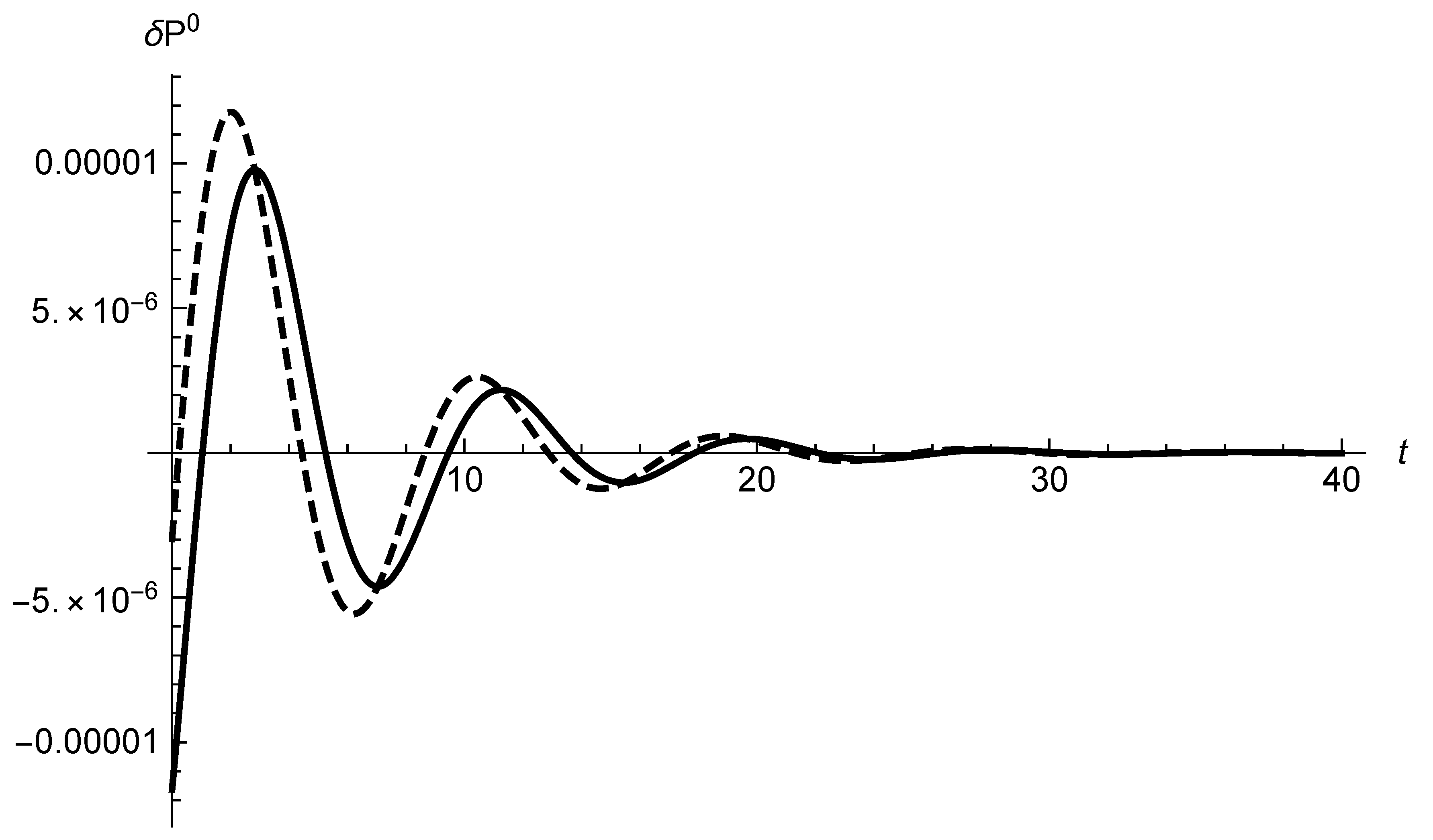
The solution given by Equation (75) may be compared with the one obtained directly from the numerical integration of Equation (72). In Figure 3, the continuous line represents the numerical solution, whereas Equation (75) is represented by the dashed line. In the numerical solution, the function was obtained by considering the full expression of the Zerilli potential, and the boundary conditions are exactly the same as considered in the case of axial perturbations. As before, the numerical solution was obtained considering and in the boundary conditions for Equation (57). We believe that the errors in the approximate analytic solution, compared to the numerical solution, are due to the approximation made in Equation (57), where we neglected the Zerilli potential in the limit . In Figure 3, we consider the initial instant of time of the perturbation. The time evolution of the energy of the perturbation is stable, since the gravitational energy of the perturbation is damped in the course of time, as shown in Figure 4.
6. Final Remarks
In this paper, we obtain the expression of the gravitational energy of the perturbations due the quasinormal modes in the Schwarzschild space-time. The expressions given by (34) and (75) hold in the limit and depend on the integers n and l. The variation in space and time of these quantities are displayed in Figure 1, Figure 2, Figure 3 and Figure 4. These are the major results of the present analysis. The dependence on the coordinate r in expressions (34) and (75) is due to the very nature of the QNM. The functions and diverge at spacelike infinity, which is a feature of the QNM. However, the perturbation is assumed to be localized and does not make sense in the limit . In our understanding, the axial and polar quasinormal perturbations represent ripples in the space-time geometry, as they do represent in the metric formulation of general relativity. However, the physical description and results displayed in Figure 1, Figure 2, Figure 3 and Figure 4 can only be obtained in the TEGR, since the the gravitational energy–momentum given by Equations (8) and (11) cannot be established in the standard formulation of general relativity.
One conclusion is that the gravitational energy of the black hole oscillates. However, since the energy of the perturbations is concentrated far from the event horizon, as shown in Figure 1 and Figure 3, we conclude that the mass of the black hole does not vary in time, i.e., the mass of the black hole (restricted to interior of the event horizon) neither increases nor decreases with time. Figure 2 and Figure 4 show that energy of the perturbations rapidly decays for large instants of time. Here, we make a distinction between the gravitational energy of the black hole (the zeroth component of the gravitational energy–momentum 4-vector ) and the mass of the black hole (an invariant of the Poincaré group, ). Note, in addition, that m is the mass of the black hole established in a frame where the black hole is at rest. In view of these considerations, we may conclude that the energy of the perturbations is a non-local effect, since it takes place sufficiently far from the event horizon. We may conjecture that the farther one is from the black hole, i.e., the farther an external perturbation is imparted to the black hole, the more energy is required to perturb it.
The dependence of expressions (34) and (75) on the integers n and l implies a discretization of the energy perturbations. This discretization must be further investigated. However, it is known that the very discretization of the QNM leads to a discretization of the area of the black hole’s event horizon [20]. A possible interplay between the discretizations of the energy perturbations and of the area of the black hole is an issue of relevant interest.
The flux of gravitational radiation emitted in the process of damping of the quasinormal modes of a Schwarzschild black hole is investigated in [21,22,23], by means of the Landau–Lifshitz pseudotensor [24], assuming that at large distances from the black hole the space-time perturbation is represented by a plane gravitational wave. The analysis in the latter references was made assuming . In the present investigation, the expression for the flux of gravitational radiation given by Equation (9) is invariant under coordinate transformations, in contrast to the pseudotensors, which are coordinate dependent expressions. It would be interesting to address a specific physical configuration, such as the collision of two black holes, and compare the energy radiated after the collision: (i) by means of Equation (39); and (ii) through the approach based on the latter references, in the context of the Landau–Lifshitz pseudotensor. This issue will be addressed elsewhere.
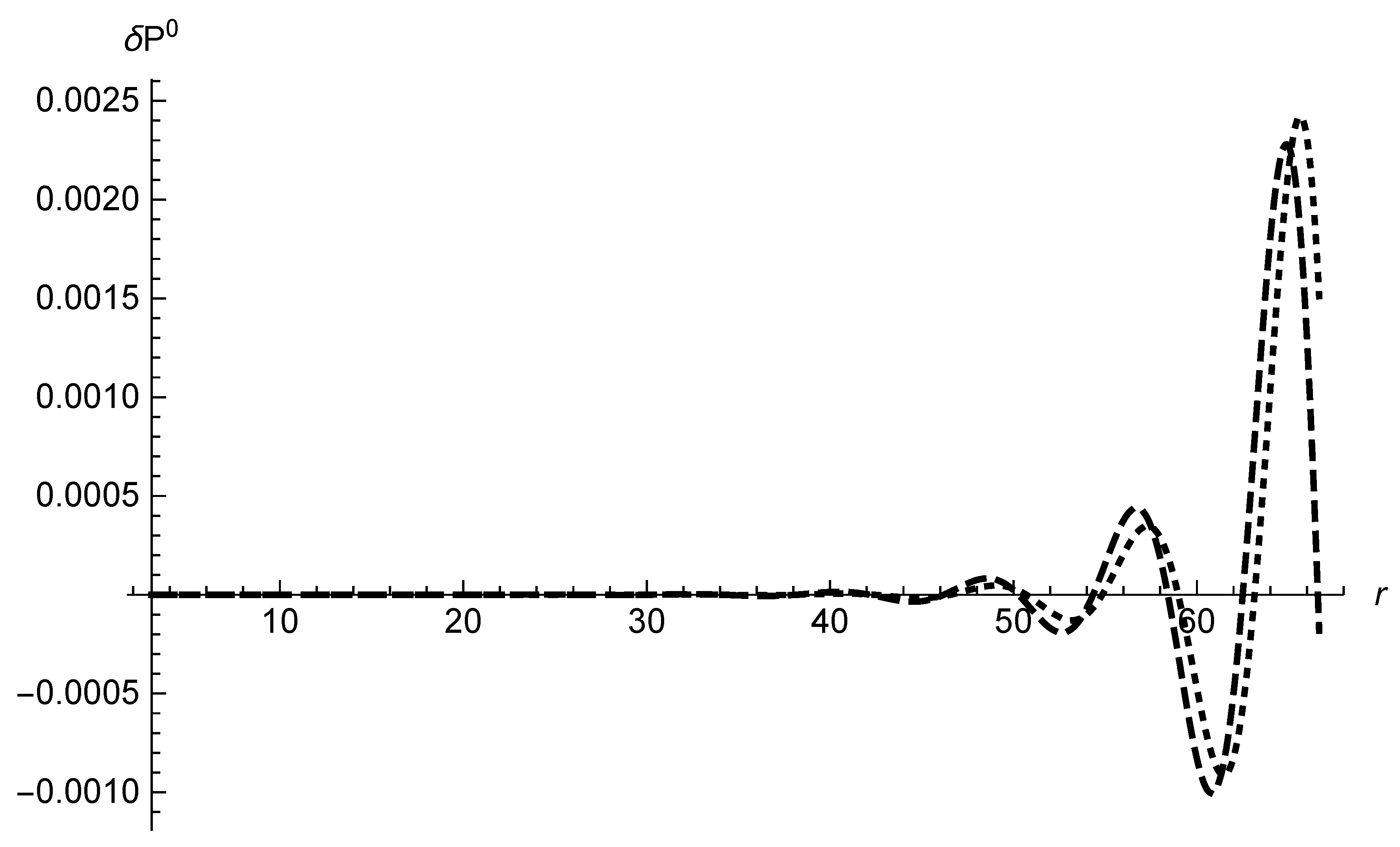
The amplitude A in the function arises as a constant of integration in the solutions of Equations (19) and (57). Let us consider the tortoise coordinate . If we make , then it is easy to see that . Therefore, there is an arbitrariness in the establishment of the amplitude A. Since the profiles of the gravitational energy perturbations in Figure 1, Figure 2, Figure 3 and Figure 4 are very similar, with a suitable choice of amplitudes, we may locally enhance the similarity between the two perturbations, as shown in Figure 5. Note that is dimensionless in the axial perturbation but has dimension (of distance) in the polar perturbation. However, the similarities between the two perturbations are very clear.
The procedure presented in this article may also be applied to extended formulations of gravity, namely, the f(T) type theories. In some of these approaches, there are proposals for the gravitational energy (see, e.g., [25,26,27,28,29]). There are various motivations to address such extended theories, for instance the analysis of the dark energy and dark matter problems, the problem of singularities of black holes, and the investigation of the degrees of freedom carried by gravitational waves. The analysis of the gravitational energy perturbations in these extended frameworks is, of course, of relevant interest.
Author Contributions
Conceptualization, The four authors contributed to the conceptualization; Formal analysis, The four authors contributes to the formal analysis; Investigation, S.U., F.L.C. and K.H.C.C.-B.; Methodology, S.U., F.L.C. and K.H.C.C.-B.; Software, F.L.C.; Supervision, J.W.M.; Writing–original draft, J.W.M.; Writing–review & editing, J.W.M. All authors have read and agreed to the published version of the manuscript.
Funding
This work received no funding other than the regular institutional support from Universidade de Brasília and Universidade Federal do Oeste do Pará.
Institutional Review Board Statement
Not applicable.
Informed Consent Statement
Not applicable.
Data Availability Statement
Not applicable.
Conflicts of Interest
There is no conflict of interest, of any kind, in the development and conclusion of this work.
References
- Nollert, H.-P. Quasinormal modes: The characteristic ‘sound’ of black holes and neutron stars. Class. Quantum Grav. 1999, 16, R159. [Google Scholar]
- Kokkotas, K.D.; Schmidt, B.G. Quasi-Normal Modes of Stars and Black Holes. Living Rev. Rel. 1999, 2, 2. [Google Scholar]
- Chandrasekhar, S. Colloquium at Syracuse University; Syracuse University: Syracuse, NY, USA, 1992. [Google Scholar]
- Schutz, B.F.; Will, C.W. Black hole normal modes—A semianalytic approach. Astrophys. J. 1985, 291, L33. [Google Scholar]
- Maluf, J.W. The gravitational energy-momentum tensor and the gravitational pressure. Ann. Phys. 2005, 14, 723. [Google Scholar]
- Maluf, J.W.; da Rocha-Neto, J.F.; Toríbio, T.M.L.; Castello-Branco, K.H. Energy and angular momentum of the gravitational field in the teleparallel geometry. Phys. Rev. D 2002, 65, 124001. [Google Scholar]
- Maluf, J.W.; Faria, F.F.; Castello-Branco, K.H. The gravitational energy–momentum flux. Class. Quantum Grav. 2003, 20, 4683. [Google Scholar]
- Maluf, J.W.; Faria, F.F. On gravitational radiation and the energy flux of matter. Ann. Phys. 2004, 13, 604. [Google Scholar]
- Maluf, J.W. The teleparallel equivalent of general relativity. Ann. Phys. 2013, 525, 339. [Google Scholar]
- Regge, T.; Wheeler, J.A. Stability of a Schwarzschild singularity. Phys. Rev. 1957, 108, 1063. [Google Scholar]
- Iyer, S.; Will, C.M. Black-hole normal modes: A WKB approach. I. Foundations and application of a higher-order WKB analysis of potential-barrier scattering. Phys. Rev. D 1987, 35, 3621. [Google Scholar]
- Iyer, S. Black-hole normal modes: A WKB approach. II. Schwarzschild black holes. Phys. Rev. D 1987, 35, 3632. [Google Scholar]
- Konoplya, R.A. Quasinormal behavior of the D-dimensional Schwarzschild black hole and the higher order WKB approach. Phys. Rev. D 2003, 68, 024018. [Google Scholar]
- Berti, E.; Cardoso, V.; Starinets, A.O. Quasinormal modes of black holes and black branes. Class. Quantum Grav. 2009, 26, 163001. [Google Scholar]
- Nollert, H.-P.; Schmidt, G.G. Quasinormal modes of Schwarzschild black holes: Defined and calculated via Laplace transformation. Phys. Rev. D 1992, 45, 2617. [Google Scholar]
- Maluf, J.W.; Faria, F.F.; Ulhoa, S.C. On reference frames in spacetime and gravitational energy in freely falling frames. Class. Quantum Grav. 2007, 24, 2743. [Google Scholar]
- Hehl, F.H.; Lemke, J.; Mielke, E.W. Two Lectures on Fermions and Gravity. In Geometry and Theoretical Physics; Debrus, J., Hirshfeld, A.C., Eds.; Springer: Berlin/Heidelberg, Germany, 1991. [Google Scholar]
- Zerilli, F.J. Effective potential for even parity Regge-Wheeler gravitational perturbation equations. Phys. Rev. Lett. 1970, 24, 737. [Google Scholar]
- Chandrasekhar, S.; Detweiler, S. The Quasi-Normal Modes of the Schwarzschild Black Hole. Proc. R. Soc. Lond. A Math. Phys. Sci. 1975, 344, 441. [Google Scholar]
- Maggiore, M. Physical Interpretation of the Spectrum of Black Hole Quasinormal Modes. Phys. Rev. Lett. 2008, 100, 141301. [Google Scholar] [PubMed] [Green Version]
- Cunningham, C.T.; Price, R.H.; Moncrief, V. Radiation from collapsing relativistic stars. I. Linearized odd-parity radiation. Astrophys. J. 1978, 224, 643. [Google Scholar]
- Nagar, A.; Rezolla, L. Gauge-invariant Non-spherical Metric Perturbations of Schwarzschild Black-Hole Spacetimes. Class. Quantum Grav. 2005, 22, R167. [Google Scholar]
- Nakano, H.; Ioka, K. Second Order Quasi-Normal Mode of the Schwarzschild Black Hole. Phys. Rev. D 2007, 76, 084007. [Google Scholar] [CrossRef] [Green Version]
- Landau, L.D.; Lifshitz, E.M. The Classical Theory of Fields, 4th ed.; Pergamon Press: Oxford, UK, 1975. [Google Scholar]
- Capozziello, S.; Capriolo, M.; Transirico, M. The gravitation energy–momentum pseudotensor: The cases of F(R) and F(T) gravity. Int. J. Geom. Methods Mod. Phys. 2018, 15, 1850164. [Google Scholar]
- Capozziello, S.; Capriolo, M.; Transirico, M. The gravitational energy-momentum pseudo-tensor of higher-order theories of gravity. Ann. Phys. 2017, 529, 1600376. [Google Scholar] [CrossRef] [Green Version]
- Capozziello, S.; Capriolo, M.; Caso, L. Gravitational waves in higher order teleparallel gravity. Class. Quantum Grav. 2020, 37, 235013. [Google Scholar]
- Capozziello, S.; Capriolo, M.; Caso, L. Weak field limit and gravitational waves in higher-order gravity. Int. J. Geom. Methods Mod. Phys. 2019, 16, 1950047. [Google Scholar]
- Ulhoa, S.C.; Spaniol, E.P. On the Gravitational Energy-momentum Vector in f(T) Theories. Int. J. Mod. Phys. D 2013, 22, 1350069. [Google Scholar] [CrossRef] [Green Version]
Figure 1.
Comparison between the real parts of the gravitational energy of the axial perturbation. The continuous line represents the values of the numerical integration of the energy, whereas the dashed line represents the values obtained from the approximate analytic expression (34). The parameters used are , . The frequency was required to be the fundamental frequency (, ), obtained from the third-order WKB method. The data represent the initial instant of time of the perturbation, i.e., .

Figure 2.
Comparison between the real parts of the gravitational energy of the axial perturbation, as a function of time. The continuous line represents the values of the numerical integration of the energy, whereas the dashed line represents the values obtained from the approximate analytic expression (34). The parameters used are , . The frequency was required to be the fundamental frequency (, ), obtained from the third-order WKB method. The radius of integration was chosen to be , in natural units.

Figure 3.
Comparison between the real parts of the gravitational energy of the polar perturbation. The continuous line represents the numerical value of the evaluation, and the dashed line corresponds to the value resulting of the approximate analytic expression (75). The parameters used in the analysis are , , and the frequency considered is the fundamental one (, ) , obtained by means of the third-order WKB method. The data represent the initial instant of time of the perturbation, i.e., .

Figure 4.
Comparison between the real parts of the gravitational energy of the polar perturbation. The continuous line represents the numerical value of the evaluation, and the dashed line corresponds to the value resulting of the approximate analytic expression (75). The parameters used in the analysis are , , and the frequency considered is the fundamental one (, ) , obtained by means of the third-order WKB method. The integration is made on a surface of radius , in natural units.

Figure 5.
Comparison between the real parts of the gravitational energy of the perturbations. The dashed line represents the numerical expression of the energy for the axial perturbations and the dotted line represents the numerical energy of the polar perturbations. In natural units (whenever necessary), we have , , , and the frequency (fundamental, ()) is , obtained by means of the third-order WKB method. The data represent the initial instant of time of the perturbations, i.e., .

Publisher’s Note: MDPI stays neutral with regard to jurisdictional claims in published maps and institutional affiliations. |
© 2021 by the authors. Licensee MDPI, Basel, Switzerland. This article is an open access article distributed under the terms and conditions of the Creative Commons Attribution (CC BY) license (https://creativecommons.org/licenses/by/4.0/).
Share and Cite
MDPI and ACS Style
Maluf, J.W.; Ulhoa, S.; Carneiro, F.L.; Castello-Branco, K.H.C. Perturbations of the Gravitational Energy in the TEGR: Quasinormal Modes of the Schwarzschild Black Hole. Universe 2021, 7, 100. https://doi.org/10.3390/universe7040100
AMA Style
Maluf JW, Ulhoa S, Carneiro FL, Castello-Branco KHC. Perturbations of the Gravitational Energy in the TEGR: Quasinormal Modes of the Schwarzschild Black Hole. Universe. 2021; 7(4):100. https://doi.org/10.3390/universe7040100
Chicago/Turabian StyleMaluf, José Wadih, Sérgio Ulhoa, Fernando Lessa Carneiro, and Karlúcio H. C. Castello-Branco. 2021. "Perturbations of the Gravitational Energy in the TEGR: Quasinormal Modes of the Schwarzschild Black Hole" Universe 7, no. 4: 100. https://doi.org/10.3390/universe7040100
Note that from the first issue of 2016, this journal uses article numbers instead of page numbers. See further details here.