Remotely Sensed Derived Land Surface Temperature (LST) as a Proxy for Air Temperature and Thermal Comfort at a Small Geographical Scale

Abstract

Urban Heat Islands (UHIs) and Urban Cool Islands (UCIs) can be measured by means of in situ measurements and interpolation methods, which often require densely distributed networks of sensors and can be time-consuming, expensive and in many cases infeasible. The use of satellite data to estimate Land Surface Temperature (LST) and spectral indices such as the Normalized Difference Vegetation Index (NDVI) has emerged in the last decade as a promising technique to map Surface Urban Heat Islands (SUHIs), primarily at large geographical scales. Furthermore, thermal comfort, the subjective perception and experience of humans of micro-climates, is also an important component of UHIs. It remains unanswered whether LST can be used to predict thermal comfort. The objective of this study is to evaluate the accuracy of remotely sensed data, including a derived LST, at a small geographical scale, in the case study of King Abdulaziz University (KAU) campus (Jeddah, Saudi Arabia) and four surrounding neighborhoods. We evaluate the potential use of LST estimates as proxy for air temperature (T_air) and thermal comfort. We estimate LST based on Landsat-8 measurements, T_air and other climatological parameters by means of in situ measurements and subjective thermal comfort by means of a Physiological Equivalent Temperature (PET) model. We find a significant correlation (r = 0.45, p < 0.001) between LST and mean T_air and the compatibility of LST and T_air as equivalent measures using Bland-Altman analysis. We evaluate several models with LST, NDVI, and Normalized Difference Built-up Index (NDBI) as data inputs to proxy T_air and find that they achieve error rates across metrics that are two orders of magnitude below that of a comparison with LST and T_air alone. We also find that, using only remotely sensed data, including LST, NDVI, and NDBI, random forest classifiers can detect sites with “very hot” classification of thermal comfort nearly as effectively as estimates using in situ data, with one such model attaining an F1 score of 0.65. This study demonstrates the potential use of remotely sensed measurements to infer the Physiological Equivalent Temperature (PET) and subjective thermal comfort at small geographical scales as well as the impacts of land cover and land use characteristics on UHI and UCI. Such insights are fundamental for sustainable urban planning and would contribute enormously to urban planning that considers people’s well-being and comfort.

1. Introduction

Urban Heat Island (UHI) occurs when the atmospheric temperature in urban areas is higher compared to surrounding rural settings [1]. It results, in part, from heat that is released, stored or re-radiated from anthropogenic heat sources in the city [2]. In contrast to the UHI effect, Urban Cool Islands (UCIs) are also often observed in urban areas, for example, in arid and semi-arid regions, when irrigated or green surfaces create “cool islands” or an “oasis” effect [3] within urban settings. UCIs are attributed, in part, to evapotranspiration from wet surfaces and transpiration from plant leaves, whereby radiant energy driving the surface energy balance is converted into latent heat [4], resulting in “cool islands” characterized by a temperature that is between 2.5–6 °C lower relative to their surroundings [5], most prominently during daytime [6,7]. UHI and UCI have immense impacts on the atmosphere, ecology, environment, economy, society and public health [8]. Understanding the spatial patterns and characteristics of UHIs and UCIs is fundamental for urban or regional planning that aims to promote citizens’ well-being, for example, through the development of parks and green belts in hot and arid regions [9].

Many factors affect the intensity of UHIs and UCIs. For example, surface albedo plays a crucial role in creating cooler “islands” [10], while the reflectance and roughness of land use and land cover (LULC) [11,12] and the composition, configuration, complexity, intensity [13,14,15,16,17], morphology and heterogeneity [18] of objects on Earth, such as buildings, including their materials [19] and heights [20], affect the intensity of the UHI. In general, urban artificial impervious surfaces (e.g., asphalt roads and residential, commercial and industrial land use) are often characterized by higher LSTs compared to natural LULC types such as bodies of water, urban parks and green spaces [17,18,19,21]. Micro-climate conditions, including wind speed and cloud cover, also impact the intensity of the UHI effect [22].

The difference between the temperature observed in urban compared to rural areas may be observed on the surface level or in the air (atmosphere) above [23,24]. UHI is typically measured or characterized by means of fixed stations, mobile traverse, remote sensing, vertical sensing or energy balance [25]. At the urban canopy layer, UHIs can be measured using in situ measurements collected at locations surrounded by average or “typical” conditions that represent the urban terrain, usually at 2 m above ground and ideally with sufficient radiation shielding and ventilation [26].

1.1. Surface Urban Heat Island (SUHI) and Land Surface Temperature (LST)

While in situ measurements can provide an accurate recording of the climatological conditions in a given location, to fully leverage in situ measurements to understand the extent and characteristics of UHI, there is a need for a densely distributed network of sensors throughout the urban environment, which can be time-consuming, expensive and in many cases infeasible [27]. As a result, more affordable and feasible methods have been developed to estimate inter- and intra-urban temperature variations, primarily at the surface level (Surface Urban Heat Island (SUHI)).

SUHI refers to the thermal differences between artificial surfaces in urban areas compared to natural surfaces in the surrounding rural areas, which result, in part, from differences in the absorption and reflectance characteristics of the surfaces [28]. Previous studies suggest that SUHI generally follows similar trends to atmospheric UHI [29,30,31]. According to [1], the scale and pace of urbanization processes are linked with changes in average surface temperature and SUHI.

SUHI can be characterized according to Land Surface Temperature (LST) measurements using airborne or satellite thermal infrared remote sensing measurements [28,32]. LST refers to the “surface radiometric temperature” [33] or the “radiative ‘skin’ temperature” [34] as measured according to the radiation emitted from Earth in the Thermal Infrared channel (TIR) [35]. Previous studies show that LST is closely related to air temperature [36,37], although this relationship varies by geography, topography and characteristics of the land use and land cover (LULC) [30,31].

Both, UHI and SUHI phenomena have been examined in the literature at different geographical scales, including at the level of continents [38,39,40], countries [41], cities and metropolitan areas [13,42] and increasingly at micro-scales [43,44]. To illustrate, [45] examines the impacts of urban functional zones and spatial heterogeneity on LST in Beijing, China; Temporal changes in LST as a result of urban redevelopments in Lyon, France where investigated by [46]; and the impacts of different types of LULC patterns on SUHI variations in Bangkok, Thailand, where evaluated by [47]. Similarly, the impacts of the composition of different types of land cover on SUHI have been examined in the cases of Austin and San Antonio, Texas [48] and Portland, Oregon [49]. Recently, [50] estimated patterns of LST over King Abdulaziz University campus (Jeddah, Saudi Arabia), demonstrating the potential of Landsat-derived LST estimates to map long-term changes of the UHI phenomenon at a geographical scale of a university campus.

1.2. Thermal Comfort

While UHI and UCI are typically defined according to observed variations in air temperature, both phenomena have immense impacts on people’s well-being and thermal comfort, which are predominantly associated with the UHI phenomenon [51]. Thermal comfort refers to the subjective sensation or satisfaction with the thermal environment [52,53]. According to this definition, any deviation from a thermal comfort range could result in a discomfort sensation [54]. Especially during periods of heat stress in warm-weather cities, the UHI effect may have a debilitating effect on the health and activity of people in the urban area [55] and their thermal comfort [56]. Thermal comfort is not only a factor of air temperature, but also a factor of other climatological conditions such as wind speed and air humidity [57,58], solar radiation [59] and duration of direct sun [60].

In addition, thermal comfort is impacted by LULC characteristics. Greenery areas, for example, urban parks, trees and gardens, or water bodies [61], can increase the livability of urban areas and people’s comfort from both physiological and psychological perspectives [62,63,64].

While thermal comfort can be measured using direct interviews or questionnaires, several numeric indices have been developed to estimate the “real feel” or the sensation of the temperature, including the temperature-humidity index (THI) (originally developed by [65]), the wet bulb-globe temperature index (WBGT) [66], the physiological equivalent temperature (PET) [67] and the universal thermal climatic index (UTCI) [68]. Of these, PET is especially advantageous because it is a universal index useful in both hot and colder climates, irrespective of clothing and metabolic activity; it is calculated based on thermo-physiological variables, which capture humans’ sensation of climate without relying on subjective measures, and is measured in °C, which make it easy to interpolate [69].

1.3. Study Objectives

In parallel to the advancements in remotely sensed derived LST estimations, several approaches have been proposed to validate the accuracy of LST estimations. Validation with in situ measurements is probably the most commonly used method to assess the accuracy of LST [29,70]. Only a limited number of studies evaluate the potential of LST as a proxy for thermal comfort. Existing studies look, for example, at the potential of LST for estimating Temperature Humidity Index (THI) [71] or for heat stress mapping [72].

In this study, we evaluate the relationship between remotely sensed derived LST, in situ measurements and thermal comfort in the case study of King Abdulaziz University (KAU) campus (Jeddah, Saudi Arabia). We estimate LST using Landsat-8 observations and compare LST’s derived spatial patterns against in situ climatological measurements and thermal comfort. The objectives of this study are as follows: (1) to validate the methodology presented in [50] to map the extent and spatial patterns of LST in the case study of KAU campus and the surrounding residential neighborhoods; (2) to evaluate the relationship between LST and climatological in situ measurements; (3) to evaluate the association between T_air, LST and PET (as an indicator of thermal comfort); (4) to evaluate the relation of T_air, LST and PET to LULC; (5) to demonstrate the impact of different types of land cover and land use on micro-climate variations.

We now turn to describe the methodology adopted in this study to assess the UHI using remotely sensed measurements and in situ measurements (Section 2). In Section 3 we describe the results, followed by a discussion and conclusion (Section 4 and Section 5, respectively).

2. Materials and Methods

2.1. Study Area

The analysis was performed on King Abdulaziz University (KAU) campus, Jeddah, Saudi Arabia, and four surrounding neighborhoods: Al Sulaymaniyah from the north, Abruq Ar Rughamah from the east, Al Jami’ah from the south, and from the west Al Fayha’a (Figure 1).

2.2. Data

2.2.1. Estimating Land Surface Temperature (LST)

Remotely sensed observations collected by the Landsat constellation of satellites are ideal for LST estimations thanks to the thermal infrared radiometers carried by the Landsat 5, 7 and 8 satellites, which make their data suitable for LST estimations, including for characterization of UHI. In this study, we derived LST estimations from Band 10 (Thermal infrared (TIR1), resampled from 100 m to 30 m, 10.60–11.19 µm) of Landsat-8 observations (a detailed description of the methodology is provided in Appendix A). The in situ measurements were carried out between 3–9 September 2020; however, during this period there were no overpasses of Landsat-8 over the Area of Interest (AOI). We thus relied on four Landsat-8 overpasses that collected imagery closest to the time the in situ measurements were collected: 12 August, 28 August, 13 September, and 19 September 2020.

For analyzing the correspondence between LST and LULC, we calculated the median LST for these four Landsat-8 overpasses (12 August, 28 August, 13 September, 29 September 2020). For a direct comparison with in situ and PET measurements (collected from 3 through 9 September), temporal precision was more important, given weather dynamics, so we calculated the mean of the Landsat-8 overpasses immediately preceding (28 August 2020) and succeeding (13 September 2020) the dates of in situ collection.

2.2.2. Climatological In Situ Measurements

We collected climatological measurements using a WTH600-E-KIT Wireless Weather Station Kit (http://www.extech.com/products/WTH600-E-KIT (accessed on 9 April 2021)), a versatile and mobile climate measuring toolkit ideal for taking climatological measurements at ground level (1.5 m off the ground). Collected measurements include temperature (in Celsius, with an accuracy of +/− 0.5 °C), relative humidity (the ratio of water vapor in the air versus the quantity of water vapor the air could theoretically hold at the given temperature, measured in %RH, with an accuracy of +/− 3 %RH), air pressure (measured in hectopascals with an accuracy of +/− 4 hPa), wind speed and direction (measured in km/h and cardinal directions, respectively).

Climatological measurements were collected during a seven-day period from 3 September to 9 September 2020, four times a day: morning (3:30 a.m.–5 a.m.), midday (12 p.m.–2:30 p.m.), afternoon (3:30 p.m.–5 p.m.) and evening (8 p.m.–10 p.m.) (all times local: UTC +3.0). We collected measurements in 20 locations (12 locations on campus and 8 outside of campus that were publicly accessible (i.e., by car or by foot) (Figure 1), with each measurement approximately 10 min in length. These locations represent a diverse range of land cover and land use types, including green spaces, densely built areas, bare land, paved areas, etc. (photos of these locations are provided in Figure 2). In each location we collected measurements at five measurement sites (a center location and four satellite locations, each 100 m to the north, south, east and west), totaling 100 measurement sites. Measurements were collected during the day under sunny and shaded conditions (e.g., under trees, fences, and buildings).

In total, 3405 measurements were collected; however, a few observations contained outlier values, including some possible data entry errors, which were cleaned and filtered. Observations that had a relative humidity measurement outside 0–100% or an air temperature measurement 5 standard deviations above or below the mean were omitted from analysis. After filtering, 3393 measurements remained for use in analysis.

2.2.3. Thermal Indices

Like [73], we calculate the Physiological Equivalent Temperature (PET) index based on the Radiation on the Human Body (RayMan) model [74]. RayMan is a freely available radiation and human bioclimate model (available for download at: https://www.urbanclimate.net/rayman/ (accessed on 9 April 2021)). PET allows for understanding the effect of complex outdoor weather factors by estimating an equivalent “indoor” temperature that simulates the same thermal effect given environmental variables (we provide the PET formula in Appendix B).

The RayMan model calculates the amount of heat flow that would be produced given certain outdoor conditions, including levels of radiation from direct and reflected sunlight that affect mean radiant temperature, a key influence on the human heat-balance equation [74]. The model then determines what air temperature would be required in the reference indoor environment to achieve the same heat flow, and the resulting temperature is the PET. The RayMan model simulates short- and long-wave radiation flux densities from the three dimensional surroundings [75]. According to [74], the radiation fluxes are most important for the human energy balance of the human body and the resulting thermal index PET, especially during summer. The model considers all simple and complex environments with their radiation properties (albedo and emissivity). It estimates the radiation fluxes and the effects of clouds on short-wave radiation fluxes [76].

We calculated PET with the RayMan model using the data collected in situ as inputs, including date, time of day, air temperature, relative humidity, wind speed and estimated cloud coverage. We set the location to be centered on Jeddah (21° N, 39° E) and at sea level. For the biometric data, we assumed an average height (1.67 m), weight (75.3 kg) and age (31 years) (relying on https://www.who.int/ncds/surveillance/steps/2005_SaudiArabia_STEPS_Report_EN.pdf (accessed on 9 April 2021)). We assumed a light layer of clothing and light activity (akin to walking).

We also calculated a “heat index” based on [77,78]:

$$\begin{array}{c}\mathrm{HI}=-42.379+2.04901523\mathrm{T}+10.14333127\mathrm{R}-0.22475541\mathrm{TR}-6.83783\ast {10}^{-3}{T}^2-5.481717\\ \ast {10}^{-2}{R}^2+1.22874\ast {10}^{-3}{T}^2\mathrm{R}+8.5282\ast {10}^{-4}T{R}^2-1.99\ast {10}^{-6}{T}^2{R}^2\end{array}$$

(1)

where T = ambient dry bulb temperature (°F) and R = relative humidity (integer percentage).

2.2.4. Fulcrum

All measurements of field surveys were recorded into a mobile application survey platform, Fulcrum (https://www.fulcrumapp.com (accessed on 9 April 2021)) (provided by Fulcrum for evaluation for this study). Fulcrum was downloaded onto both OS and Android devices and synched with a web application.

2.2.5. Spectral Indices

We also assessed the relation between LST, in situ measurements, PET and LULC, namely green vegetation and built-up land cover. While several spectral indices have been proposed in the literature for capturing green vegetation and built-up land cover, it was not the objective of this study to compare between the different spectral indices. We thus relied on two of the most used spectral indices: The Normalized Difference Vegetation Index (NDVI) [79] to capture vegetation and the Normalized Difference Built-up Index (NDBI) [80] to capture built-up land cover.

NDVI expresses the relation between red visible light (which is typically absorbed by a plant’s chlorophyll) and near-infrared wavelength (which is scattered by the leaf’s mesophyll structure). It is computed as

$$\mathrm{NDVI}=\left(\mathrm{NIR}-\mathrm{RED}\right)/\left(\mathrm{NIR}+\mathrm{RED}\right),$$

(2)

where NIR is the near-infrared wavelength and RED is the red wavelength. The values of NDVI range between (−1) and (+1).

NDBI expresses the relation between the medium-infrared and the near-infrared wavelengths. It is computed as

$$\mathrm{NDBI}=\left(\mathrm{MIR}-\mathrm{NIR}\right)/\left(\mathrm{MIR}+\mathrm{NIR}\right),$$

(3)

where MIR is the medium-infrared and NIR is the near-infrared wavelength. The index assumes a higher reflectance of built-up areas in the medium-infrared wavelength range than in the near-infrared.

To examine the relation between spatial patterns and characteristics of T_air and remotely sensed data (LST, NDVI and NDBI) we overlaid the locations of the in situ measurement sites with the corresponding Landsat pixels. We used the Spearman Rank measure to calculate the correlations between these measures (given its robustness with non-normally distributed data [81]) and the Bland-Altman method [82] to assess the agreement between them. For the Bland-Altman analysis, we set a threshold so that 95% of the data within +/− two standard deviations of the mean difference between both methods would indicate a viable correspondence. For this analysis, we only included observations collected from 12 p.m. to 1 p.m. local time (n = 869), which are the closest in time to Landsat’s overpass (i.e., around 10:50 a.m. local time); however, we used all available in situ observations after the filtering described in Section 2.2.2 for general comparative analysis (n = 3393).

To capture the nonlinear interactions of the remotely sensed and in situ covariates, we employed multiple linear regression (Ordinary Least Squares) and a few simple nonlinear models, including logistic regression, Bayesian ridge regression [83,84], random forest regression [85], and gradient boosted machines (XGB) [86], across combinations of LST, NDVI, NDBI against T_air and PET (see Appendix C).

For validation metrics, we used the median error (MdE) for accuracy, the median absolute deviation for precision (MdAD) and the root mean squared error (equivalently, root mean squared deviation, RMSD) for uncertainty [87]. We ran 5-fold cross-validation and evaluated the metrics and correlation on only the validation fold of each run.

Finally, we investigated the ability of LST and these spectral indices to detect “very hot” locations (namely UHI) and compared these patterns against the in situ measurements. We assigned levels of thermal comfort to measurement sites based on median PET value. We followed the scale presented with the RayMan model and presented in [88] (

Table 1. Levels of thermal comfort based on Physiological Equivalent Temperature (PET) values [88].

PET (°C)	Thermal Perception	Grade of Physical Stress
>41	Very hot	Extreme heat stress
35–41	Hot	Strong heat stress
29–35	Warm	Moderate heat stress
23–29	Slightly warm	Slight heat stress
18–23	Comfortable	No thermal stress
13–18	Slightly cool	Slight cold stress
8–13	Cool	Moderate cold stress
4–8	Cold	Strong cold stress
≤4	Very cold	Extreme cold stress

).

The median PET temperatures during the data collection fell in the Warm, Hot, and Very Hot scale range (Figure 3). We therefore aimed to isolate “very hot locations” (i.e., where the median PET temperature was above 41 °C) in order to create two relatively comparable sample sets: “very hot” (n = 57) and the rest of the observations (n = 43).

With these two classes identified, we evaluated a set of logistic regression and random forest classifiers to evaluate the potential to infer these classes based on a range of data inputs collected either from the in situ data or from Landsat-8. We used a harmonic mean (i.e., F1 score) as the evaluation metric:

$$F1score=\frac{TP}{TP+\frac{1}{2}\left(FP+FN\right)}$$

(4)

where TP are True Positives, FP are False Positives and FN are False Negatives. As with the LST and T_air comparison, we conducted 5-fold stratified cross-validation and only evaluated performance on the test fold of each iteration.

3. Results

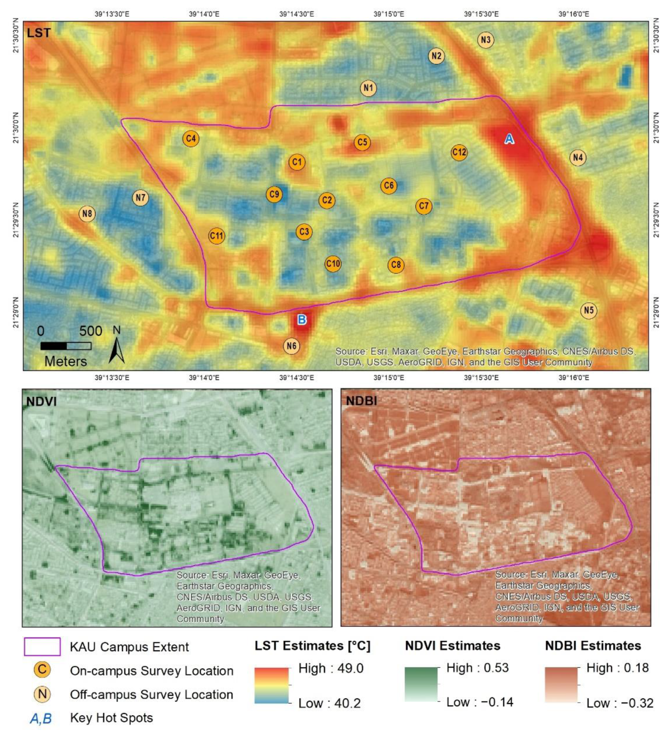
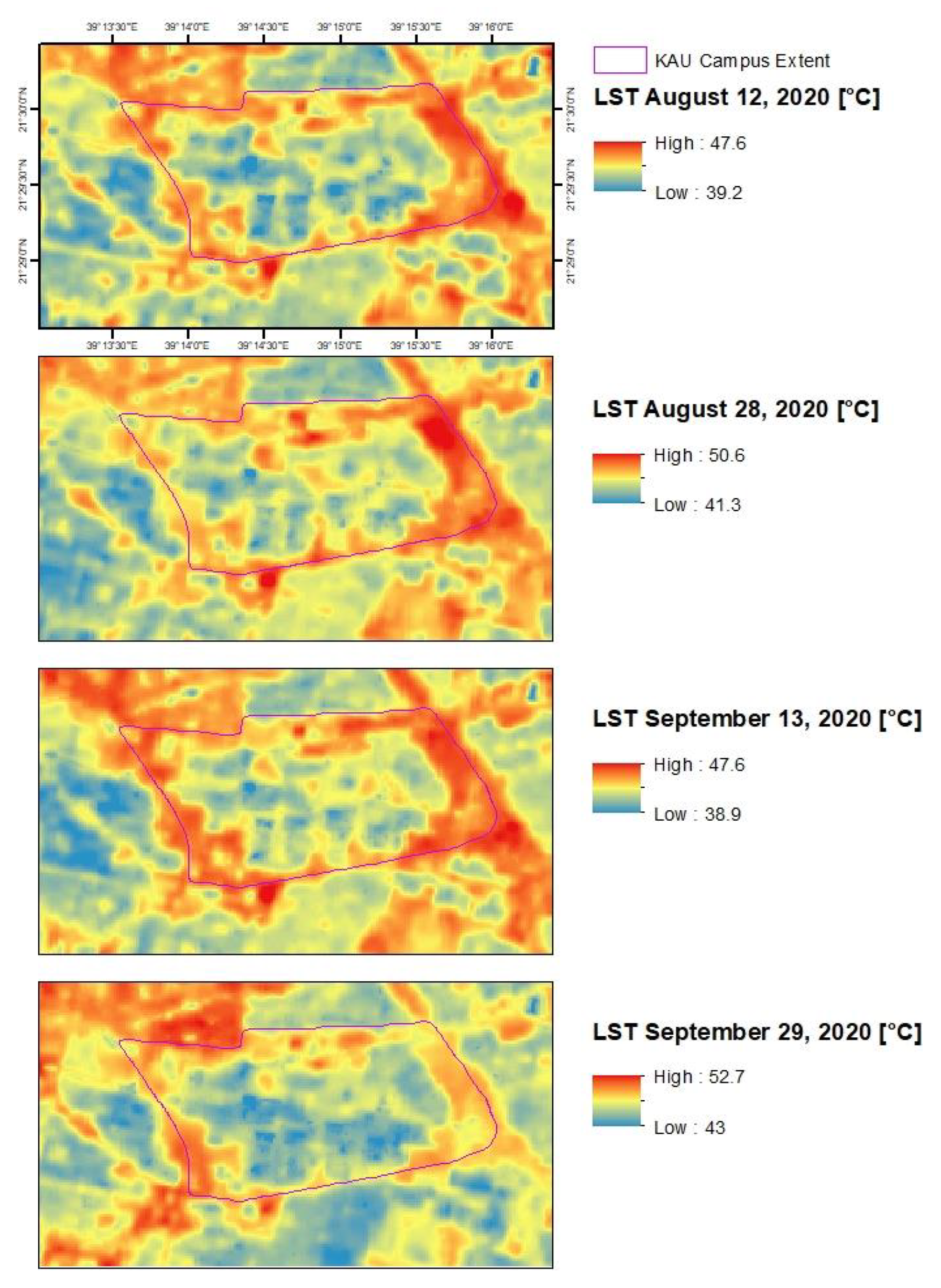
3.1. Spatial Patterns of LST Estimations

The analysis revealed variations in the spatial patterns of LST across the study area, which we relate to the distribution and characteristics of the LULC, including green vegetation, bare land, paved surfaces, built-up structures and building materials. LST varied between the four Landsat-8 overpasses; the highest LST in the study area (calculated as the average LST value of all pixels within the study area) was measured on 13 September and the lowest on 29 September (48.4 °C and 43 °C, respectively).

For comparison between LST, NDVI and NDBI, we calculated the median LST value of each pixel in the four Landsat-8 scenes to create a single composite scene. As expected, green spaces were characterized by lower LST compared to paved built surfaces and bare land (Figure 4 presents the distribution of NDVI and NDBI (bottom left and right, respectively) compared to LST (top)). For example, the LST measured over the bare land area east of the staff housing (Figure 4, area A) was 48.1 °C, while the lowest LST was measured around the green roundabout for the administrative entrance (around 41 °C, Figure 4, area C9), an area characterized by natural grass, mature trees, palms, shrubs, groundcover and grass.

Outside of campus, the highest LST (48.8 °C) was measured over Al Jamea Plaza shopping center south of campus (Figure 4, area B), which we attribute to the construction materials of the shopping center (namely rough textured concrete, stone, glass and metal). The association between LST and LULC was also reflected in the correlation we found between LST, NDVI and NDBI. Namely, as LST increased, NDVI decreased and NDBI increased (r= −0.45 and r = 0.6, respectively, p < 0.001 for both).

A comparison of the four Landsat overpass LST values across the 100 measurement sites shows that the lowest mean temperature was measured on 29 September (42.33 °C), while the highest mean temperature was measured on 13 September (47.82 °C) (

Table 2. Mean LST across the 100 measurement sites per Landsat-8 overpass.

Overpass Date
	12 August 2020	28 August 2020	13 September 2020	29 September 2020	Composite 1
Measurement locations	Mean: 43.30 °C StdDev: 1.18 °C	Mean: 45.52 °C StdDev: 1.32 °C	Mean: 47.82 °C StdDev: 1.34 °C	Mean: 42.33 °C StdDev: 1.14 °C	Mean: 46.67 °C StdDev: 1.28 °C

¹ Composite is calculated as the mean value of the 28 August and 13 September overpasses.

provides the average derived LST from each Landsat overpass).

Of the four Landsat overpasses, the overpasses on 28 August and 13 September over the AOI are the closest to the time the in situ measurements were collected. To evaluate the similarity in the climatological conditions between the time of the two Landsat overpasses (28 August and 13 September) and the time of the in situ measurements (3 September to 9 September), we obtained climatological data from the General Authority of Meteorology & Environmental Protection, Saudi Arabia, for additional validation. These measurements were collected at the Jeddah KAIA meteorological station (21°42′37.0″ N 39°11′12.0″ E)—the closest official station to the research area. We obtained recordings of maximum temperature, maximum humidity and maximum wind speed during the research period. As shown in

Table 3. Independent measurements of temperature, humidity and wind that demonstrate weather during data collection consistent with days of the Landsat-8 overpass (28 August and 13 September).

Climate Measure	3 September	4 September	5 September	6 September	7 September	8 September	9 September	Average 3–9 September	8 August	13 September	Average 28 August to 13 September
Max Temp (°C)	36.8	39.0	39.6	37.4	37.2	36.2	39.0	37.9	37.4	41.8	39.6
Max Humidity (%)	66	71	73	83	80	75	80	75.4	74	76	75
Mean Wind (km/h)	6	5	4	4	4	6	3	4.6	5	8	6.5

, the maximum temperature, humidity and wind speed recorded between 3 September and 9 September were relatively similar to the average recordings on 28 August and 13 September (the time of the two Landsat overpasses). The average maximum temperature during the week the in situ measurements were collected was 37.9 °C (SD = 1.13 °C) compared to an average of 39.6 °C on 28 August and 13 September. The relative humidity was also similar (around 75%). These findings confirm that the climatological conditions during the time of the two Landsat overpasses did not differ much from those observed during the week the in situ measurements were collected. In this study, we thus relied on the average LST measurements collected on 28 August and 13 September.

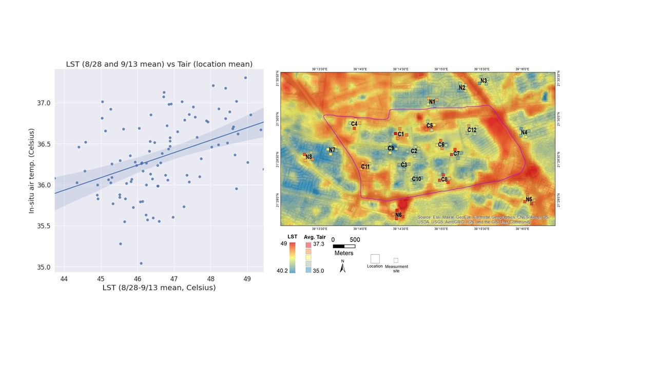
3.2. Spatial patterns of LST and Air Temperature (T_air)

Analysis of the air temperature (T_air) measured across the 100 measurement sites reveals similar patterns to those observed with the LST measurements, which we relate to the characteristics of the LULC and micro-conditions of the measurement sites.

Figure 5 presents the distributions of T_air for all observations (n = 3393). Several trends are apparent, including the diurnal variation of the mean temperature, which ranges from 32.75 °C in the morning and 32.46 °C in the evening to 34.66 °C in the afternoon and 38.64 °C at midday. As expected, T_air was lower in sites characterized by green vegetation and higher in areas covered with built-up or paved surfaces and bare land. This is indicated by a significant correlation between the average T_air, NDVI and NDBI (r = −0.29, p = 0.003 and r = 0.36, p < 0.001, respectively).

One of the key objectives of this study was to examine the potential utilization of remotely sensed derived LST to estimate T_air and thermal comfort. We did not attempt to conduct an exact calibration of the two measures; rather, we wanted to understand their relative compatibility to detect spatial patterns of temperature variations. We used the Bland-Altman method to compare the mean and the difference of T_air and LST. This method allowed us to identify acceptable parameters and any potential biases; it is often used in the literature for assessing agreement when simple correlation is not adequate [89]. Figure 6 presents a comparison (scatterplot) of the mean and the difference between T_air and LST across 869 measurements collected between 12 p.m. and 2 p.m. local time (closest to the Landsat-8 overpass window time that data were collected). The results suggest that the distribution of the difference is normal (per Shapiro-Wilk test, p = 0.719) and that 96% of the observations are within 1.96 standard deviations of the mean difference (i.e., above the 95% threshold). There is a bias evident such that the overall LST temperatures were on average 6.54 °C above that of T_air, whereas if the differences were due to stochastic error alone, we would expect the average to be zero. This bias tends to increase as the temperature increases. While we did not find a statistically significant correlation between LST and in situ data collected between 12 p.m. and 2 p.m., there was a significant correlation (r = 0.45, p < 0.001) between LST and the mean T_air for each measurement site (n = 100) across all observations (n = 3393) (Figure 7).

We also evaluated the correlation between the LST derived from each of the two Landsat overpasses, with the mean T_air measured for each measurement day (i.e., 3 September to 9 September). The results show a significant correlation between the LST we derived from each Landsat overpass individually (23 August and 13 September) and the T_air that was measured during four of the measurement days (5 September, 7 September, 8 September and 9 September). For LST derived based on the 28 August Landsat overpass, this correlation ranges between r = 0.27, p = 0.006 and r = 0.35, p < 0.001 (when compared against the T_air measured on 8 September and 7 September, respectively); for LST derived from the Landsat overpass on 13 September, this correlation ranges between r = 0.29, p = 0.002 and r = 0.36, p < 0.001 (when compared against the T_air measured on 7 September, and 9 September, respectively). When looking at different times of the day T_air was measured, we found the strongest correlation between LST derived from the Landsat overpass on 28 August and the T_air measured on 8 September in the evening (between 7 p.m. and 9 p.m., r = 0.49, p < 0.001). We explain this finding by the fact that LST is likely higher than T_air during the daytime and relatively lower or comparable to T_air during the later times of the day, when the near surface atmosphere is more stable.

As explained above, in this study we sought to understand the relative compatibility between LST, T_air and PET in detecting spatial patterns of temperature variations. As illustrated in Figure 8 (a visual assessment of the correspondence between the distribution of T_air,_max per measurement site against LST estimations), there was a general visual correspondence between LST and T_air patterns. For example, the green space in the roundabout leading to campus administrative buildings (Figure 8, C9) and the green space near the women’s campus (Figure 8, C10), which are characterized by the lowest LST (41 °C and 42.9 °C, respectively), are also among the coolest locations as indicated by T_air (T_air,max is on average 43.1 °C and 42.5 °C in these locations, respectively).

Next, we evaluated the overall relationships between LST and T_air as an indication of spatial characteristics contributing to UHI or UCI. Because the objective was to examine spatial (rather than temporal) similarities, we calculated the mean value of the in situ measurements collected throughout the entire day (n = 3393) and evaluated their relationship with LST and other potential nonlinear interactions among several variables. Determining optimal modeling techniques was not the primary aim of this analysis, so model evaluation and tuning were not explored in-depth; however, as noted, these techniques offer insight into the relationship of remotely sensed data and in situ measurements, including subtle nonlinear relationships. The results therefore show “adjusted” LST values as per the various models and input data, which are compared to T_air. To serve as a baseline assessment, a comparison between LST (non-adjusted) and T_air values yielded the following metrics (all units are in degrees Celsius):

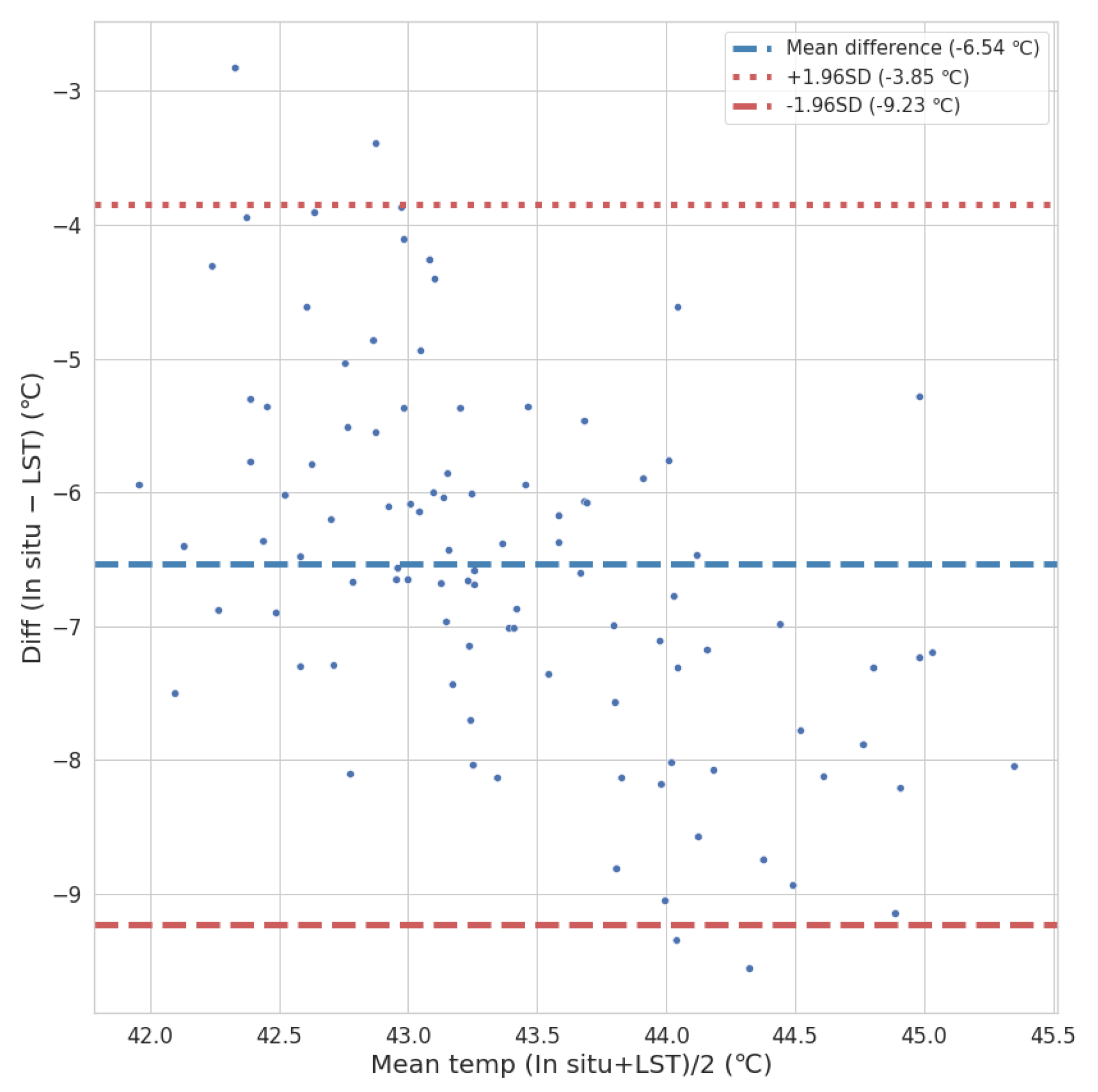
• Accuracy via Median Error (MdE): −10.30281
• Precision via Median Absolute Deviation (MdAD): 0.73945
• Uncertainty via Root Mean Squared Difference (RMSD): 10.39249

The results of these experiments (

Table 4. Performance of various models to adjust LST (as calculated by the mean of 28 August and September values) vs. the in situ air temperature (as calculated by the mean T_air for 100 measurement sites across all hours of the day, n = 3393). Predicting in situ temperature with LST + NDBI with Random Forest (RF) had the lowest error (MdE): −0.00071. LST + NDVI with RF had the greatest precision (MdAD): 0.28195. LST + NDBI + NDVI with RF had the lowest uncertainty (RMSD): 0.43689.

Covariates	Results
	Multiple Regression (OLS)	Bayesian Ridge Regression	Random Forest Regression (RF)	XGBoost
LST	MdE: 0.00899	MdE: 0.00763	MdE: 0.06445	MdE: 0.06939
	MdAD: 0.32680	MdAD: 0.33245	MdAD: 0.33256	MdAD: 0.36972
	RMSD: 0.45234	RMSD: 0.45324	RMSD: 0.50124	RMSD: 0.55704
LST + NDBI	MdE: 0.00920	MdE: −0.00596	MdE: 0.00071	MdE: −0.00458
	MdAD: 0.29650	MdAD: 0.32716	MdAD: 0.30350	MdAD: 0.37120
	RMSD: 0.45724	RMSD: 0.45738	RMSD: 0.44736	RMSD: 0.46745
LST + NDVI	MdE: 0.02020	MdE: 0.02479	MdE: 0.01321	MdE: −0.00904
	MdAD: 0.31834	MdAD: 0.33382	MdAD: 0.28195	MdAD: 0.31588
	RMSD: 0.46866	RMSD: 0.46594	RMSD: 0.46163	RMSD: 0.48696
LST + NDBI + NDVI	MdE: 0.01115	MdE: 0.00891	MdE: 0.00792	MdE: 0.00874
	MdAD: 0.31269	MdAD: 0.34037	MdAD: 0.30645	MdAD: 0.35008
	RMSD: 0.48220	RMSD: 0.46355	RMSD: 0.43689	RMSD: 0.46911

) suggest that, overall, the four evaluated methods performed relatively similarly across data inputs and methods, indicating a consistent association between LST and T_air. However, the more complex models (Random Forest and XGBoost) predicted an adjusted LST value closer to the actual T_air, particularly with the addition of NDVI and NDBI as inputs. Namely, LST combined with NDBI and NDVI inputs, adjusted with a nonlinear model, was a relatively strong predictor of T_air (LST + NDBI with Random Forest had the lowest MdE at 0.00071, LST + NDVI with Random Forest had the lowest MdAD at 0.28195, and LST + NDBI + NDVI with Random Forest had the lowest RMSD at 0.43689). A Spearman correlation test of this model’s output (i.e., Random Forest model with LST + NDBI + NDVI inputs) with T_air resulted in an R² of 0.41 (p < 0.001), suggesting that this model explained 41% of the variance in T_air.

Additionally, the analysis across all data and methods to determine an “adjusted” LST performed much better across the error metrics (i.e., the adjusted LST values were closer to T_air) than the baseline of LST and T_air alone, indicating that using models that capture unobserved dynamics or latent relationships across spatial and temporal dimensions and covariates provide an effective way to proxy T_air, as long as proper guards against over-fitting are observed (i.e., results hold up on out-of-sample data).

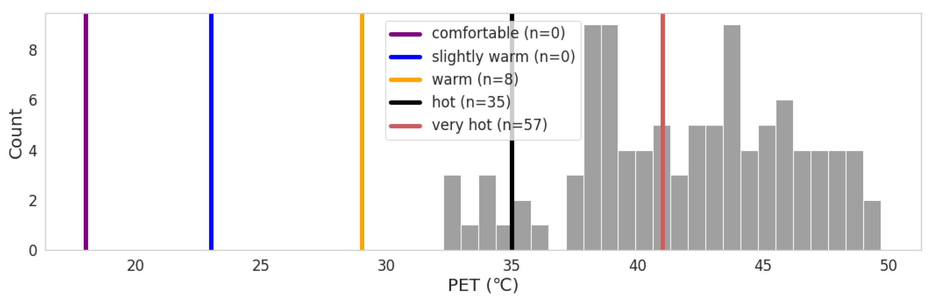
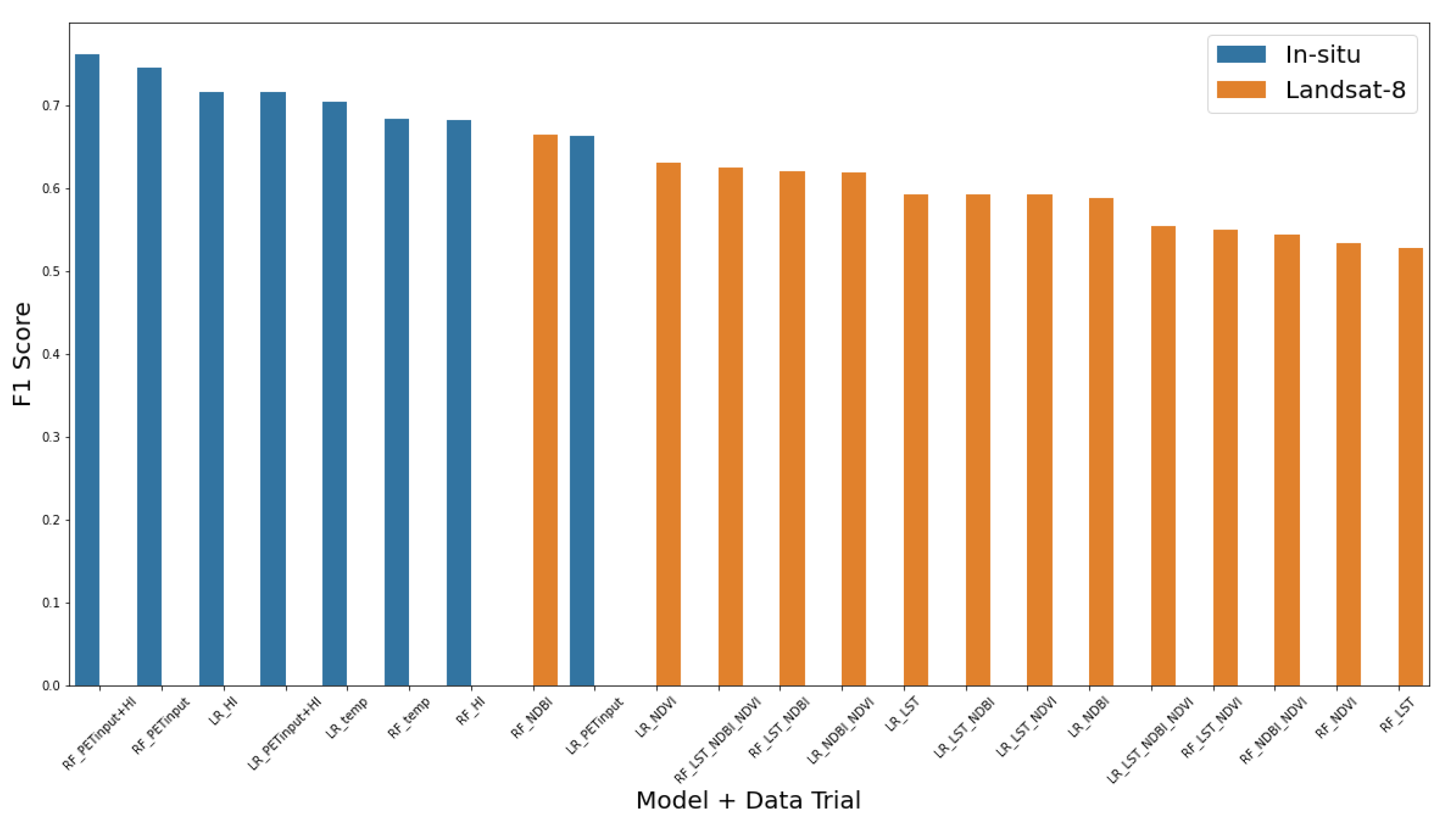
3.3. Inferring Thermal Comfort with In Situ and Landsat-8 Data

Next, we evaluated the association between T_air and the Physiological Equivalent Temperature (PET) as a heat-balance model of the human body. As expected, we found a strong and statistically significant correlation between PET and T_air (r = 0.95, p < 0.001). This relationship held when looking at the mean PET and T_air across all observations for each location (r = 0.73; p < 0.001), as is clearly illustrated in Figure 9a. There was also a significant correlation between PET and heat index for each location (r = 0.75, p < 0.001) (Figure 9b). This indicates that the relationship between PET and in situ measurements held over time as a general trend and lends insight into spatial characteristics of these locations. We also found that mean PET correlated with LST (the mean of 28 August and 13 September Landsat-8 overpasses), albeit at a weaker and lower statistical threshold (r = 0.23, p = 0.02) (Figure 9c). We also evaluated the association between the LST derived from the two Landsat overpasses and the daily PET measurements. The results show a significant correlation between LST and the PET measurements on 5 September, 7 September and 9 September. The correlation ranged between r = 0.22 and r = 0.29 (between LST derived from Landsat’s 28 August overpass and PET measurements from 7 September and 9 September, respectively, p = 0.03 for 7 September, and p = 0.004 for 9 September) and between r = 0.20 and r = 0.32 (between LST derived from Landsat’s 13 September overpass and PET measurements from 5 September and 9 September, respectively, p = 0.04 for 5 September and p = 0.001 for 9 September).

However, as described above, the main objective of this study was not to merely compare the absolute measurement values, but also to demonstrate the potential use of remotely sensed derived LST measures to identify “hot spots” of “uncomfortable areas”, at least according to PET. For this aim, a series of logistic regression and Random Forest models were used to infer whether a location could be categorized as “very hot” (i.e., a median PET above 41 °C). Both models were fit to in situ air temperature alone, the heat index alone, to all the inputs to the PET model (i.e., air temperature, relative humidity, wind speed, cloud coverage) and to all these inputs combined (i.e., air temperature, relative humidity, wind speed, cloud coverage, and heat index) (Figure 10). When the same models were used to infer “very hot” locations using only combinations of remotely sensed data (LST, NDBI, NDVI), they performed surprisingly well. In fact, a Random Forest model with NDBI outperformed one of the models using in situ data.

As expected, the models using in situ data performed well given that they were based on the same input data as those used in the RayMan model to develop the PET score. The best model (i.e., a Random Forest model with air temperature, relative humidity, average wind speed, cloud coverage and heat index as inputs) attained an F1 score of 0.76116. However, the top-performing model using only remote sensing data (Random Forest with NDBI) attained an F1 score of 0.66429, which was competitive with the in situ based models and even outperformed one model that used in situ data. Other variations of Random Forest using only remote sensing data performed comparably as well.

4. Discussion

Many studies have investigated the characteristics of Urban Heat Island (UHI) and the various factors that impact its spatial patterns and intensity. With the increased availability of remotely sensed satellite and airborne measurements, there is a growing interest in developing methods that utilize remotely sensed observations to estimate the characteristics and extent of UHI. Moreover, both UHI and UCI have immense impacts on people’s well-being and must be mapped and evaluated continuously to ensure sustainable development. Because in situ measurements to detect and map the distribution of UHI and UCI are not always available and are hard to collect, other sources of data and methodologies, such as using satellite data to estimate LST, have been increasingly adopted. The objective of this study was to evaluate the potential use of remotely sensed derived LST as proxy for spatial patterns of T_air and thermal comfort (PET).

We show that patterns of UHI and UCI detected by satellite measurements can be used to identify UHI and UCI. We found a clear relationship between the built environment, climatological measures, measures of thermal comfort (PET) and, importantly, an indication that remotely sensed data, such as LST and various spectral indices, can characterize thermal comfort at micro-scales at a performance level comparable to that of in situ data.

We found a significant positive correlation between T_air and LST (r = 0.45, p < 0.001). Despite the temporal inconsistency between the collection of the LST data and the in situ measurements, we were still able to find an agreement between these two measures via the Bland-Alman method. We also detected some systemic bias, such that the overall LST temperatures were on average 6.54 °C above that of T_air. This bias tended to increase as the temperature increased. According to [90], T_air is often lower than LST, especially when vegetation cover is low to moderate; over non-vegetated surfaces the difference may even exceed 20 °C.

We also evaluated the relationship between LST and T_air using several regression models. The Random Forest model performed best; however, all models fared far better than just the baseline comparison between LST and T_air, attaining error rates two orders of magnitude lower, indicating their potential to capture latent dynamics in the data that can be exploited to approximate T_air. Nonparametric models such as Random Forests are capable of combining the benefits of interpretability and flexibility [91]. Here, we show that Random Forest Regression can be used to infer T_air with LST, NDBI and NDVI, which together can predict up to 41% of the variation of T_air. These findings support other studies of more complex models, such as Random Forest, to infer T_air from LST [92,93].

Furthermore, we evaluated the potential use of LST to infer thermal comfort, i.e., the subjective perception of the thermal conditions by humans. We estimated thermal comfort using the Physiological Equivalent Temperature (PET) as a heat-balance model of the human body. Similar to [94], our results support the validity of PET as a measure of thermal comfort in local spatial and temporal (intra-day) scales and highlight its value in investigating the effects of UHI and UCI in micro-urban spaces. While the correlation between LST and PET was relatively low (r = 0.23, p = 0.02), a Random Forest regression was able to infer “very hot” locations using only combinations of remotely sensed data (LST, NDBI, NDVI). By classifying in situ measurement sites according to their median PET values and identifying “very hot” sites, we demonstrated that both logistic regression and Random Forest classifiers were able to infer levels of thermal comfort using a few input variables collected in situ, with the top model attaining an F1 score of 0.761157. This further affirms that PET might be useful in quantifying UHI and UCI effects using some basic measurements and a model, such as the RayMan model, for PET. What was perhaps more interesting was our finding that Random Forest classifiers using only remote sensing data (LST, NDBI, NDVI) were able to achieve comparable results (e.g., a Random Forest classifier using only NDBI attained an F1 score of 0.664286), demonstrating the potential to investigate predictions of thermal comfort at micro-scales using satellite data. Given the cost and inability to scale ground-based instrumentation, this is an encouraging sign, although more data and studies are needed.

Finally, we evaluated the relationship between in situ measurements, remotely sensed data and LULC characteristics. The results show variations in spatial patterns of LST that were closely related to the characteristics of the LULC, including the spatial distribution of green vegetated spaces, bare land, paved surfaces, built-up structures, and building materials. The spatial resolution of Landsat-8 (30 m) was high enough to distinguish between the temperature of sites separated by only a few hundred meters and characterized by different types of land use and land cover (LULC) (e.g., green spaces and parking lots). Similar to [95], we found that green spaces were characterized by lower LST compared to paved built surfaces and bare land (the difference between the maximum and minimum LST across the 100 measurement sites was 5.5 °C). This trend was indicated by a high and significant correlation between LST and two spectral indices representing green vegetation (NDVI) and built-up land cover (NDBI) (r = −0.45 and r = 0.6, respectively, p < 0.001 for both). These results align with previous studies that show a positive correlation between LST and NDBI and a negative correlation with NDVI [96,97,98]. To illustrate, [99] found a negative correlation between LST and NDVI (up to r = −0.63) and a positive correlation with NDBI (up to r = 0.67).

As expected, and similar to [100], we found that T_air was lower in sites located in areas covered with green vegetation and higher in areas covered with built-up or paved surfaces and bare land. However, we found a lower correlation between the average T_air, NDVI and NDBI (r = −0.29, p = 0.003 and r = 0.36, p < 0.001, respectively). We explain this relatively low correlation by the fact that the in situ temperature measurements represent a single location and are subject to various micro-climate conditions that are more significant than the overall vegetation cover around the location.

We note a few limitations to this study. First, in situ measurements were collected over a period of one week. Although the climate of Jeddah, Saudi Arabia, does not tend to vary much between seasons, a future study should also look at seasonal variations in predicting T_air. Second, the validation of in situ data and remotely sensed data is best done with observations that are precisely aligned. Third, this study was conducted in Saudi Arabia, which is an arid region. A future study should evaluate the potential of LST to predict T_air and thermal comfort in diverse types of climatological regions, including semi-arid and tropical. Fourth, in this study we used constant emissivity parameters to estimate LST. However, these parameters may differ by region and be subject to the land characteristics. While this was not the aim of the current study, a future study could investigate methods to improve the accuracy of T_air predictions by identifying the optimal emissivity parameters.

5. Conclusions

Rapid urbanization processes together with temperature increases due to climate change are expected to result in an intensification of the Urban Heat Island (UHI) phenomenon by approximately 1 °C per decade, impacting the environment, ecology, biodiversity and people’s well-being. Monitoring the extent and characteristics of the UHI is fundamental for the maintenance of sustainable urban systems and allows human settlements to be more inclusive, safe, resilient, and sustainable.

Traditional methods to measure UHI include the use of in situ measurements of climatological parameters, which are often collected ad hoc and are expensive and sparse. The increasing availability of new sources of medium spatial resolution remotely sensed satellite measurements in the last decade has triggered the development of new methods to estimate the Land Surface Temperature (LST) as a proxy for UHI. However, the majority of these studies evaluate the potential of these measurements to estimate the temperature of the air (T_air) at large geographical scales, due in part to the potential limitations due to the spatial resolution of the data. Furthermore, most studies utilize satellite measurements to estimate LST rather than the subjective thermal comfort, or sensation, of the thermal environment.

Three main conclusions arise from this study:

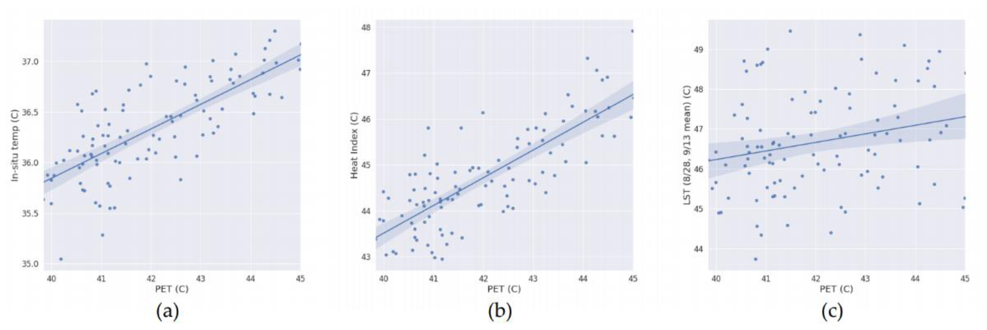
• There is a significant correlation between LST, T_air and PET, which are all also related to LULC characteristics (including those indicated by NDVI and NDBI spectral indices).
• There is a correspondence between spatial patterns of UHI and UCI, as detected by means of remotely sensed and in situ observations.
• Logistic regression and Random Forest models can be used to infer if a location is categorized as “very hot” (per PET), even when just considering LST, NDBI and NDVI.

Urban planning, mitigation and intervention efforts can help mitigate the UHI effect. This can be done, for example, by increasing green vegetation in urban areas or by planting trees along roadsides in dry areas (e.g., [101]). However, as noted by [102], there is no one mitigation solution that fits all cases, and any mitigation must consider the specific characteristics of the specific geographic area.

References

1. Chen, M.; Zhou, Y.; Hu, M.; Zhou, Y. Influence of Urban Scale and Urban Expansion on the Urban Heat Island Effect in Metropolitan Areas: Case Study of Beijing–Tianjin–Hebei Urban Agglomeration. Remote Sens. 2020, 12, 3491. [Google Scholar] [CrossRef]
2. Memon, R.A.; Leung, D.Y.C.; Chunho, L. A Review on the Generation, Determination and Mitigation of Urban Heat Island. J. Environ. Sci. 2008, 20, 120–128. [Google Scholar] [CrossRef]
3. Wen, L.J.; Lü, S.H.; Chen, S.Q.; Meng, X.H.; Bao, Y. Numerical Simulation of Cold Island Effect in Jinta Oasis Summer. Plateau Meteorol. 2005, 24, 865–871. [Google Scholar]
4. Shashua-Bar, L.; Pearlmutter, D.; Erell, E. The Influence of Trees and Grass on Outdoor Thermal Comfort in a Hot-Arid Environment. Int. J. Climatol. 2011, 31, 1498–1506. [Google Scholar] [CrossRef]
5. Rasul, A.; Balzter, H.; Smith, C.; Remedios, J.; Adamu, B.; Sobrino, J.A.; Srivanit, M.; Weng, Q. A Review on Remote Sensing of Urban Heat and Cool Islands. Land 2017, 6, 38. [Google Scholar] [CrossRef] [Green Version]
6. Yang, X.; Li, Y.; Luo, Z.; Chan, P.W. The Urban Cool Island Phenomenon in a High-rise High-density City and Its Mechanisms. Int. J. Climatol. 2017, 37, 890–904. [Google Scholar] [CrossRef]
7. Haashemi, S.; Weng, Q.; Darvishi, A.; Alavipanah, S.K. Seasonal Variations of the Surface Urban Heat Island in a Semi-Arid City. Remote Sens. 2016, 8, 352. [Google Scholar] [CrossRef] [Green Version]
8. Maimaitiyiming, M.; Ghulam, A.; Tiyip, T.; Pla, F.; Latorre-Carmona, P.; Halik, Ü.; Sawut, M.; Caetano, M. Effects of Green Space Spatial Pattern on Land Surface Temperature: Implications for Sustainable Urban Planning and Climate Change Adaptation. ISPRS J. Photogramm. Remote Sens. 2014, 89, 59–66. [Google Scholar] [CrossRef] [Green Version]
9. Mirzaei, M.; Verrelst, J.; Arbabi, M.; Shaklabadi, Z.; Lotfizadeh, M. Urban Heat Island Monitoring and Impacts on Citizen’s General Health Status in Isfahan Metropolis: A Remote Sensing and Field Survey Approach. Remote Sens. 2020, 12, 1350. [Google Scholar] [CrossRef]
10. Saneinejad, S.; Moonen, P.; Carmeliet, J. Comparative Assessment of Various Heat Island Mitigation Measures. Build. Environ. 2014, 73, 162–170. [Google Scholar] [CrossRef]
11. Deng, Y.; Wang, S.; Bai, X.; Tian, Y.; Wu, L.; Xiao, J.; Chen, F.; Qian, Q. Relationship among Land Surface Temperature and LUCC, NDVI in Typical Karst Area. Sci. Rep. 2018, 8, 1–12. [Google Scholar] [CrossRef]
12. Bokaie, M.; Zarkesh, M.K.; Arasteh, P.D.; Hosseini, A. Assessment of Urban Heat Island Based on the Relationship between Land Surface Temperature and Land Use/Land Cover in Tehran. Sustain. Cities Soc. 2016, 23, 94–104. [Google Scholar] [CrossRef]
13. Zhou, W.; Huang, G.; Cadenasso, M.L. Does Spatial Configuration Matter? Understanding the Effects of Land Cover Pattern on Land Surface Temperature in Urban Landscapes. Landsc. Urban Plan. 2011, 102, 54–63. [Google Scholar] [CrossRef]
14. Weng, Q.; Liu, H.; Liang, B.; Lu, D. The Spatial Variations of Urban Land Surface Temperatures: Pertinent Factors, Zoning Effect, and Seasonal Variability. IEEE J. Sel. Top. Appl. Earth Obs. Remote Sens. 2008, 1, 154–166. [Google Scholar] [CrossRef]
15. Mallick, J.; Kant, Y.; Bharath, B.D. Estimation of Land Surface Temperature over Delhi Using Landsat-7 ETM+. J Ind Geophys Union 2008, 12, 131–140. [Google Scholar]
16. Zhibin, R.; Haifeng, Z.; Xingyuan, H.; Dan, Z.; Xingyang, Y. Estimation of the Relationship between Urban Vegetation Configuration and Land Surface Temperature with Remote Sensing. J. Indian Soc. Remote Sens. 2015, 43, 89–100. [Google Scholar] [CrossRef]
17. Rotem-Mindali, O.; Michael, Y.; Helman, D.; Lensky, I.M. The Role of Local Land-Use on the Urban Heat Island Effect of Tel Aviv as Assessed from Satellite Remote Sensing. Appl. Geogr. 2015, 56, 145–153. [Google Scholar] [CrossRef]
18. Guo, G.; Zhou, X.; Wu, Z.; Xiao, R.; Chen, Y. Characterizing the Impact of Urban Morphology Heterogeneity on Land Surface Temperature in Guangzhou, China. Environ. Model. Softw. 2016, 84, 427–439. [Google Scholar] [CrossRef]
19. Abutaleb, K.; Ngie, A.; Darwish, A.; Ahmed, M.; Arafat, S.; Ahmed, F. Assessment of Urban Heat Island Using Remotely Sensed Imagery over Greater Cairo, Egypt. Adv. Remote Sens. 2015, 4, 35. [Google Scholar] [CrossRef] [Green Version]
20. Bakarman, M.A.; Chang, J.D. The Influence of Height/Width Ratio on Urban Heat Island in Hot-Arid Climates. Procedia Eng. 2015, 118, 101–108. [Google Scholar] [CrossRef]
21. Schatz, J.; Kucharik, C.J. Seasonality of the Urban Heat Island Effect in Madison, Wisconsin. J. Appl. Meteorol. Climatol. 2014, 53, 2371–2386. [Google Scholar] [CrossRef]
22. Arnfield, A.J. Two Decades of Urban Climate Research: A Review of Turbulence, Exchanges of Energy and Water, and the Urban Heat Island. Int. J. Climatol. J. R. Meteorol. Soc. 2003, 23, 1–26. [Google Scholar] [CrossRef]
23. Fabrizi, R.; Bonafoni, S.; Biondi, R. Satellite and Ground-Based Sensors for the Urban Heat Island Analysis in the City of Rome. Remote Sens. 2010, 2, 1400–1415. [Google Scholar] [CrossRef] [Green Version]
24. Voogt, J.A.; Oke, T.R. Thermal Remote Sensing of Urban Climates. Remote Sens. Environ. 2003, 86, 370–384. [Google Scholar] [CrossRef]
25. Gartland, L.M. Heat Islands: Understanding and Mitigating Heat in Urban Areas; Routledge: London, UK, 2012; ISBN 1-136-56421-7. [Google Scholar]
26. Oke, T.R. Initial Guidance to Obtain Representative Meteorological Observations at Urban Sites; WMO: Geneva, Switzerland, 2006. [Google Scholar]
27. Mirzaei, P.A.; Haghighat, F. Approaches to Study Urban Heat Island–Abilities and Limitations. Build. Environ. 2010, 45, 2192–2201. [Google Scholar] [CrossRef]
28. Peng, S.; Piao, S.; Ciais, P.; Friedlingstein, P.; Ottle, C.; Bréon, F.-M.; Nan, H.; Zhou, L.; Myneni, R.B. Surface Urban Heat Island across 419 Global Big Cities. Environ. Sci. Technol. 2012, 46, 696–703. [Google Scholar] [CrossRef] [PubMed]
29. Göttsche, F.-M.; Olesen, F.-S.; Bork-Unkelbach, A. Validation of Land Surface Temperature Derived from MSG/SEVIRI with in Situ Measurements at Gobabeb, Namibia. Int. J. Remote Sens. 2013, 34, 3069–3083. [Google Scholar] [CrossRef]
30. Martin, M.A.; Ghent, D.; Pires, A.C.; Göttsche, F.-M.; Cermak, J.; Remedios, J.J. Comprehensive In Situ Validation of Five Satellite Land Surface Temperature Data Sets over Multiple Stations and Years. Remote Sens. 2019, 11, 479. [Google Scholar] [CrossRef] [Green Version]
31. Srivastava, P.K.; Majumdar, T.J.; Bhattacharya, A.K. Surface Temperature Estimation in Singhbhum Shear Zone of India Using Landsat-7 ETM+ Thermal Infrared Data. Adv. Space Res. 2009, 43, 1563–1574. [Google Scholar] [CrossRef]
32. Yuan, F.; Bauer, M.E. Comparison of Impervious Surface Area and Normalized Difference Vegetation Index as Indicators of Surface Urban Heat Island Effects in Landsat Imagery. Remote Sens. Environ. 2007, 106, 375–386. [Google Scholar] [CrossRef]
33. Dash, P.; Göttsche, F.-M.; Olesen, F.-S.; Fischer, H. Land Surface Temperature and Emissivity Estimation from Passive Sensor Data: Theory and Practice-Current Trends. Int. J. Remote Sens. 2002, 23, 2563–2594. [Google Scholar] [CrossRef]
34. Yang, Y.Z.; Cai, W.H.; Yang, J. Evaluation of MODIS Land Surface Temperature Data to Estimate Near-Surface Air Temperature in Northeast China. Remote Sens. 2017, 9, 410. [Google Scholar] [CrossRef] [Green Version]
35. Li, Z.-L.; Tang, B.-H.; Wu, H.; Ren, H.; Yan, G.; Wan, Z.; Trigo, I.F.; Sobrino, J.A. Satellite-Derived Land Surface Temperature: Current Status and Perspectives. Remote Sens. Environ. 2013, 131, 14–37. [Google Scholar] [CrossRef] [Green Version]
36. Soltani, A.; Sharifi, E. Daily Variation of Urban Heat Island Effect and Its Correlations to Urban Greenery: A Case Study of Adelaide. Front. Archit. Res. 2017, 6, 529–538. [Google Scholar] [CrossRef]
37. Cui, Y.Y.; de Foy, B. Seasonal Variations of the Urban Heat Island at the Surface and the Near-Surface and Reductions Due to Urban Vegetation in Mexico City. J. Appl. Meteorol. Climatol. 2012, 51, 855–868. [Google Scholar] [CrossRef]
38. Imhoff, M.L.; Zhang, P.; Wolfe, R.E.; Bounoua, L. Remote Sensing of the Urban Heat Island Effect across Biomes in the Continental USA. Remote Sens. Environ. 2010, 114, 504–513. [Google Scholar] [CrossRef] [Green Version]
39. Pinheiro, A.C.T.; Mahoney, R.; Privette, J.L.; Tucker, C.J. Development of a Daily Long Term Record of NOAA-14 AVHRR Land Surface Temperature over Africa. Remote Sens. Environ. 2006, 103, 153–164. [Google Scholar] [CrossRef]
40. Zhang, P.; Bounoua, L.; Imhoff, M.L.; Wolfe, R.E.; Thome, K. Comparison of MODIS Land Surface Temperature and Air Temperature over the Continental USA Meteorological Stations. Can. J. Remote Sens. 2014, 40, 110–122. [Google Scholar]
41. Prakash, S.; Norouzi, H. Land Surface Temperature Variability across India: A Remote Sensing Satellite Perspective. Theor. Appl. Climatol. 2020, 139, 773–784. [Google Scholar] [CrossRef]
42. Fu, P.; Weng, Q. A Time Series Analysis of Urbanization Induced Land Use and Land Cover Change and Its Impact on Land Surface Temperature with Landsat Imagery. Remote Sens. Environ. 2016, 175, 205–214. [Google Scholar] [CrossRef]
43. Jenerette, G.D.; Harlan, S.L.; Buyantuev, A.; Stefanov, W.L.; Declet-Barreto, J.; Ruddell, B.L.; Myint, S.W.; Kaplan, S.; Li, X. Micro-Scale Urban Surface Temperatures Are Related to Land-Cover Features and Residential Heat Related Health Impacts in Phoenix, AZ USA. Landsc. Ecol. 2016, 31, 745–760. [Google Scholar] [CrossRef]
44. Barbierato, E.; Bernetti, I.; Capecchi, I.; Saragosa, C. Quantifying the Impact of Trees on Land Surface Temperature: A Downscaling Algorithm at City-Scale. Eur. J. Remote Sens. 2019, 52, 74–83. [Google Scholar] [CrossRef] [Green Version]
45. Feng, Y.; Du, S.; Myint, S.W.; Shu, M. Do Urban Functional Zones Affect Land Surface Temperature Differently? A Case Study of Beijing, China. Remote Sens. 2019, 11, 1802. [Google Scholar] [CrossRef] [Green Version]
46. Renard, F.; Alonso, L.; Fitts, Y.; Hadjiosif, A.; Comby, J. Evaluation of the Effect of Urban Redevelopment on Surface Urban Heat Islands. Remote Sens. 2019, 11, 299. [Google Scholar] [CrossRef] [Green Version]
47. Keeratikasikorn, C.; Bonafoni, S. Urban Heat Island Analysis over the Land Use Zoning Plan of Bangkok by Means of Landsat 8 Imagery. Remote Sens. 2018, 10, 440. [Google Scholar] [CrossRef]
48. Zhao, C.; Jensen, J.; Weng, Q.; Weaver, R. A Geographically Weighted Regression Analysis of the Underlying Factors Related to the Surface Urban Heat Island Phenomenon. Remote Sens. 2018, 10, 1428. [Google Scholar] [CrossRef] [Green Version]
49. Moffett, K.B.; Makido, Y.; Shandas, V. Urban-Rural Surface Temperature Deviation and Intra-Urban Variations Contained by an Urban Growth Boundary. Remote Sens. 2019, 11, 2683. [Google Scholar] [CrossRef] [Green Version]
50. Addas, A.; Goldblatt, R.; Rubinyi, S. Utilizing Remotely Sensed Observations to Estimate the Urban Heat Island Effect at a Local Scale: Case Study of a University Campus. Land 2020, 9, 191. [Google Scholar] [CrossRef]
51. Qaid, A.; Lamit, H.B.; Ossen, D.R.; Shahminan, R.N.R. Urban Heat Island and Thermal Comfort Conditions at Micro-Climate Scale in a Tropical Planned City. Energy Build. 2016, 133, 577–595. [Google Scholar] [CrossRef]
52. Camuffo, D. Chapter 2 - Temperature: A Key Variable in Conservation and Thermal Comfort. In Microclimate for Cultural Heritage, 3rd ed.; Camuffo, D., Ed.; Elsevier: Amsterdam, The Netherlands, 2019; pp. 15–42. ISBN 978-0-444-64106-9. [Google Scholar]
53. Ličina, V.F.; Cheung, T.; Zhang, H.; De Dear, R.; Parkinson, T.; Arens, E.; Chun, C.; Schiavon, S.; Luo, M.; Brager, G. Development of the ASHRAE Global Thermal Comfort Database II. Build. Environ. 2018, 142, 502–512. [Google Scholar] [CrossRef] [Green Version]
54. Epstein, Y.; Moran, D.S. Thermal Comfort and the Heat Stress Indices. Ind. Health 2006, 44, 388–398. [Google Scholar] [CrossRef] [Green Version]
55. Hiemstra, J.A.; Saaroni, H.; Amorim, J.H. The Urban Heat Island: Thermal Comfort and the Role of Urban Greening. In The Urban Forest: Cultivating Green Infrastructure for People and the Environment; Pearlmutter, D., Calfapietra, C., Samson, R., O’Brien, L., Krajter Ostoić, S., Sanesi, G., Alonso del Amo, R., Eds.; Future City; Springer International Publishing: Cham, Switzerland, 2017; pp. 7–19. ISBN 978-3-319-50280-9. [Google Scholar]
56. Yang, B.; Yang, X.; Leung, L.R.; Zhong, S.; Qian, Y.; Zhao, C.; Chen, F.; Zhang, Y.; Qi, J. Modeling the Impacts of Urbanization on Summer Thermal Comfort: The Role of Urban Land Use and Anthropogenic Heat. J. Geophys. Res. Atmos. 2019, 124, 6681–6697. [Google Scholar] [CrossRef]
57. Ng, E.; Cheng, V. Urban Human Thermal Comfort in Hot and Humid Hong Kong. Energy Build. 2012, 55, 51–65. [Google Scholar] [CrossRef]
58. Lai, D.; Guo, D.; Hou, Y.; Lin, C.; Chen, Q. Studies of Outdoor Thermal Comfort in Northern China. Build. Environ. 2014, 77, 110–118. [Google Scholar] [CrossRef]
59. Nikolopoulou, M.; Baker, N.; Steemers, K. Thermal Comfort in Outdoor Urban Spaces: Understanding the Human Parameter. Sol. Energy 2001, 70, 227–235. [Google Scholar] [CrossRef]
60. Taleghani, M.; Kleerekoper, L.; Tenpierik, M.; van den Dobbelsteen, A. Outdoor Thermal Comfort within Five Different Urban Forms in the Netherlands. Build. Environ. 2015, 83, 65–78. [Google Scholar] [CrossRef]
61. Feng, L.; Zhao, M.; Zhou, Y.; Zhu, L.; Tian, H. The Seasonal and Annual Impacts of Landscape Patterns on the Urban Thermal Comfort Using Landsat. Ecol. Indic. 2020, 110, 105798. [Google Scholar] [CrossRef]
62. Coccolo, S.; Pearlmutter, D.; Kaempf, J.; Scartezzini, J.-L. Thermal Comfort Maps to Estimate the Impact of Urban Greening on the Outdoor Human Comfort. Urban For. Urban Green. 2018, 35, 91–105. [Google Scholar] [CrossRef]
63. Aram, F.; Solgi, E.; Garcia, E.H.; Mosavi, A. Urban Heat Resilience at the Time of Global Warming: Evaluating the Impact of the Urban Parks on Outdoor Thermal Comfort. Environ. Sci. Eur. 2020, 32, 117. [Google Scholar] [CrossRef]
64. Lauwaet, D.; Maiheu, B.; De Ridder, K.; Boënne, W.; Hooyberghs, H.; Demuzere, M.; Verdonck, M.-L. A New Method to Assess Fine-Scale Outdoor Thermal Comfort for Urban Agglomerations. Climate 2020, 8, 6. [Google Scholar] [CrossRef] [Green Version]
65. Thom, E.C. The Discomfort Index. Weatherwise 1959, 12, 57–61. [Google Scholar] [CrossRef]
66. Yaglou, C.P.; Minaed, D. Control of Heat Casualties at Military Training Centers. Arch Indust Health 1957, 16, 302–316. [Google Scholar]
67. Höppe, P. The Physiological Equivalent Temperature—A Universal Index for the Biometeorological Assessment of the Thermal Environment. Int. J. Biometeorol. 1999, 43, 71–75. [Google Scholar] [CrossRef]
68. Jendritzky, G.; Maarouf, A.; Staiger, H. Looking for a Universal Thermal Climate Index (UTCI) for Outdoor Applications. In Proceedings of the Windsor-Conference on Thermal Standards. 2001, pp. 5–8. Available online: https://www.researchgate.net/publication/267953388 (accessed on 9 April 2021).
69. Deb, C.; Ramachandraiah, A. The Significance of Physiological Equivalent Temperature (PET) in Outdoor Thermal Comfort Studies. Int. J. Eng. Sci. Technol. 2010, 2, 2825–2828. [Google Scholar]
70. Duan, S.B.; Li, Z.L.; Li, H.; Göttsche, F.M.; Wu, H.; Zhao, W.; Leng, P.; Zhang, X.; Coll, C. Validation of Collection 6 MODIS land surface temperature product using in situ measurements. Remote Sens. Environ. 2019, 225, 16–29. [Google Scholar] [CrossRef] [Green Version]
71. Ige, S.O.; Ajayi, V.O.; Adeyeri, O.E.; Oyekan, K.S.A. Assessing Remotely Sensed Temperature Humidity Index as Human Comfort Indicator Relative to Landuse Landcover Change in Abuja, Nigeria. Spat. Inf. Res. 2017, 25, 523–533. [Google Scholar] [CrossRef]
72. Nichol, J.E.; To, P.H. Temporal Characteristics of Thermal Satellite Images for Urban Heat Stress and Heat Island Mapping. ISPRS J. Photogramm. Remote Sens. 2012, 74, 153–162. [Google Scholar] [CrossRef]
73. Cohen, P.; Potchter, O.; Matzarakis, A. Human Thermal Perception of Coastal Mediterranean Outdoor Urban Environments. Appl. Geogr. 2013, 37, 1–10. [Google Scholar] [CrossRef]
74. Matzarakis, A.; Rutz, F.; Mayer, H. Modelling Radiation Fluxes in Simple and Complex Environments—Application of the RayMan Model. Int. J. Biometeorol. 2007, 51, 323–334. [Google Scholar] [CrossRef]
75. Matzarakis, A.; Rutz, F.; Mayer, H. Modelling Radiation Fluxes in Simple and Complex Environments: Basics of the RayMan Model. Int. J. Biometeorol. 2010, 54, 131–139. [Google Scholar] [CrossRef] [Green Version]
76. Matzarakis, A.; Rutz, F.; Mayer, H. Modelling the Thermal Bioclimate in Urban Areas with the RayMan Model. In Proceedings of the International Conference on Passive and Low Energy Architecture; Citeseer: Princeton, NJ, USA, 2006; Volume 23, pp. 449–453. [Google Scholar]
77. Rothfusz, L.P. “The Heat Index Equation (or, More Than You ever Wanted to Know about Heat Index),” Tech. Attachment, SR/SSD 90-23, NWS S. Reg. Headquarters, Forth Worth, TX. 1990. Available online: http://www.srh.noaa.gov/images/ffc/pdf/ta_htindx.PDF (accessed on 9 April 2021).
78. Steadman, R.G. The Assessment of Sultriness. Part I: A Temperature-Humidity Index Based on Human Physiology and Clothing Science. J. Appl. Meteorol. Climatol. 1979, 18, 861–873. [Google Scholar] [CrossRef] [Green Version]
79. Pettorelli, N.; Vik, J.O.; Mysterud, A.; Gaillard, J.-M.; Tucker, C.J.; Stenseth, N.C. Using the Satellite-Derived NDVI to Assess Ecological Responses to Environmental Change. Trends Ecol. Evol. 2005, 20, 503–510. [Google Scholar] [CrossRef] [PubMed]
80. Zha, Y.; Gao, J.; Ni, S. Use of Normalized Difference Built-up Index in Automatically Mapping Urban Areas from TM Imagery. Int. J. Remote Sens. 2003, 24, 583–594. [Google Scholar] [CrossRef]
81. Kokoska, S.; Zwillinger, D. CRC Standard Probability and Statistics Tables and Formulae, Student Edition; CRC Press: Boca Raton, FL, USA, 2000; ISBN 978-0-8493-0026-4. [Google Scholar]
82. Altman, D.G.; Bland, J.M. Measurement in Medicine: The Analysis of Method Comparison Studies. J. R. Stat. Soc. Ser. Stat. 1983, 32, 307–317. [Google Scholar] [CrossRef]
83. MacKay, D.J. Bayesian Interpolation. Neural Comput. 1992, 4, 415–447. [Google Scholar] [CrossRef]
84. Tipping, M.E. Sparse Bayesian Learning and the Relevance Vector Machine. J. Mach. Learn. Res. 2001, 1, 211–244. [Google Scholar]
85. Breiman, L. Random Forests. Mach. Learn. 2001, 45, 5–32. [Google Scholar] [CrossRef] [Green Version]
86. Chen, T.; Guestrin, C. Xgboost: A Scalable Tree Boosting System. In Proceedings of the 22nd ACM Sigkdd International Conference on Knowledge Discovery and Data Mining, San Francisco, CA, USA, 13–17 August 2016; pp. 785–794. [Google Scholar]
87. Guillevic, P.; Göttsche, F.; Nickeson, J.; Hulley, G.; Ghent, D.; Yu, Y.; Trigo, I.; Hook, S.; Sobrino, J.A.; Remedios, J.; et al. Land Surface Temperature Product Validation Best Practice Protocol. Version 1.1. Guillevic, P., Göttsche, F., Nickeson, J., Román, M., Eds.; Good Practices for Satellite-Derived Land Product Validation (p. 58): Land Product Validation Subgroup (WGCV/CEOS); 2018. Available online: https://lpvs.gsfc.nasa.gov/PDF/CEOS_LST_PROTOCOL_Feb2018_v1.1.0_light.pdf (accessed on 9 April 2021). [CrossRef]
88. Matzarakis, A.; Mayer, H. Another Kind of Environmental Stress: Thermal Stress. WHO Newsl. 1996, 18, 7–10. [Google Scholar]
89. Giavarina, D. Understanding Bland Altman Analysis. Biochem. Medica Biochem. Medica 2015, 25, 141–151. [Google Scholar] [CrossRef] [Green Version]
90. Good, E.J.; Ghent, D.J.; Bulgin, C.E.; Remedios, J.J. A Spatiotemporal Analysis of the Relationship between Near-Surface Air Temperature and Satellite Land Surface Temperatures Using 17 Years of Data from the ATSR Series. J. Geophys. Res. Atmos. 2017, 122, 9185–9210. [Google Scholar] [CrossRef]
91. McAlexander, R.J.; Mentch, L. Predictive Inference with Random Forests: A New Perspective on Classical Analyses. Res. Polit. 2020, 7, 2053168020905487. [Google Scholar] [CrossRef] [Green Version]
92. Xu, Y.; Knudby, A.; Ho, H.C. Estimating daily maximum air temperature from MODIS in British Columbia, Canada. Int. J. Remote Sens. 2014, 35, 8108–8121. [Google Scholar] [CrossRef]
93. Otgonbayar, M.; Atzberger, C.; Mattiuzzi, M.; Erdenedalai, A. Estimation of Climatologies of Average Monthly Air Temperature over Mongolia Using MODIS Land Surface Temperature (LST) Time Series and Machine Learning Techniques. Remote Sens. 2019, 11, 2588. [Google Scholar] [CrossRef] [Green Version]
94. Gómez, F.; Cueva, A.P.; Valcuende, M.; Matzarakis, A. Research on Ecological Design to Enhance Comfort in Open Spaces of a City (Valencia, Spain). Utility of the Physiological Equivalent Temperature (PET). Ecol. Eng. 2013, 57, 27–39. [Google Scholar] [CrossRef]
95. Gonçalves, A.; Ornellas, G.; Castro Ribeiro, A.; Maia, F.; Rocha, A.; Feliciano, M. Urban Cold and Heat Island in the City of Bragança (Portugal). Climate 2018, 6, 70. [Google Scholar] [CrossRef] [Green Version]
96. Guha, S.; Govil, H.; Dey, A.; Gill, N. Analytical Study of Land Surface Temperature with NDVI and NDBI Using Landsat 8 OLI and TIRS Data in Florence and Naples City, Italy. Eur. J. Remote Sens. 2018, 51, 667–678. [Google Scholar] [CrossRef]
97. Chen, L.; Li, M.; Huang, F.; Xu, S. Relationships of LST to NDBI and NDVI in Wuhan City Based on Landsat ETM+ Image. In Proceedings of the 2013 6th International Congress on Image and Signal Processing (CISP), Hangzhou, China, 16–18 December 2013; Volume 2, pp. 840–845. [Google Scholar]
98. Malik, M.S.; Shukla, J.P.; Mishra, S. Relationship of LST, NDBI and NDVI Using Landsat-8 Data in Kandaihimmat Watershed, Hoshangabad, India. Available online: https://core.ac.uk/download/pdf/297996963.pdf2019 (accessed on 9 April 2021).
99. Kaplan, G.; Avdan, U.; Avdan, Z.Y. Urban heat island analysis using the landsat 8 satellite data: A case study in Skopje, Macedonia. Multidiscip. Digit. Publ. Inst. Proc. 2018, 2, 358. [Google Scholar] [CrossRef] [Green Version]
100. Shiflett, S.A.; Liang, L.L.; Crum, S.M.; Feyisa, G.L.; Wang, J.; Jenerette, G.D. Variation in the Urban Vegetation, Surface Temperature, Air Temperature Nexus. Sci. Total Environ. 2017, 579, 495–505. [Google Scholar] [CrossRef]
101. Ferwati, S.; Skelhorn, C.; Shandas, V.; Makido, Y. A Comparison of Neighborhood-Scale Interventions to Alleviate Urban Heat in Doha, Qatar. Sustainability 2019, 11, 730. [Google Scholar] [CrossRef] [Green Version]
102. Makido, Y.; Hellman, D.; Shandas, V. Nature-Based Designs to Mitigate Urban Heat: The Efficacy of Green Infrastructure Treatments in Portland, Oregon. Atmosphere 2019, 10, 282. [Google Scholar] [CrossRef] [Green Version]
103. Wang, M.; Zhang, Z.; Hu, T.; Liu, X. A Practical Single-Channel Algorithm for Land Surface Temperature Retrieval: Application to Landsat Series Data. J. Geophys. Res. Atmospheres 2019, 124, 299–316. [Google Scholar] [CrossRef]
104. García-Santos, V.; Cuxart, J.; Martínez-Villagrasa, D.; Jiménez, M.A.; Simó, G. Comparison of Three Methods for Estimating Land Surface Temperature from Landsat 8-Tirs Sensor Data. Remote Sens. 2018, 10, 1450. [Google Scholar] [CrossRef] [Green Version]
105. Jiménez-Muñoz, J.C.; Cristóbal, J.; Sobrino, J.A.; Sòria, G.; Ninyerola, M.; Pons, X. Revision of the Single-Channel Algorithm for Land Surface Temperature Retrieval from Landsat Thermal-Infrared Data. IEEE Trans. Geosci. Remote Sens. 2008, 47, 339–349. [Google Scholar] [CrossRef]
106. Cristóbal, J.; Jiménez-Muñoz, J.C.; Prakash, A.; Mattar, C.; Skoković, D.; Sobrino, J.A. An Improved Single-Channel Method to Retrieve Land Surface Temperature from the Landsat-8 Thermal Band. Remote Sens. 2018, 10, 431. [Google Scholar] [CrossRef] [Green Version]
107. Sobrino, J.A.; Jiménez-Muñoz, J.C.; Paolini, L. Land Surface Temperature Retrieval from LANDSAT TM 5. Remote Sens. Environ. 2004, 90, 434–440. [Google Scholar] [CrossRef]
Figure 1. The location of the measurement sites on the King Abdulaziz University (KAU) campus, Jeddah, Saudi Arabia, and four surrounding neighborhoods: Al Sulaymaniyah, Abruq Ar Rughamah, Al Jami’ahand and Al Fayha’a.
Land 10 00410 g001
Figure 2. Survey site photos (selected measurement sites) (sites labeled ‘C’ are on campus and sites labeled ‘N’ are outside of campus as seen on the orientation map, Figure 1): (C1) Parking lot; (C2) Pedestrian walkway made of granite and precast concrete; (C3) Grassy park; (C4) Roundabout with vegetation and a water fountain made of granite; (C5) Large parking lot; (C6) Park with a central walkway made of precast concrete; (C7) Large road; (C8) Parking lot with shading structures; (C9) Brick pedestrian walkway with some vegetation; (C10) Small park with grass and trees; (C11) Large parking lot; (C12) Artificial turf field; (N1) Local neighborhood street; (N2) Parking lot with trees; (N3) Local neighborhood street; (N4) Playground with no vegetation; (N5) Park with small grassy patches; (N6) Main road; (N7) Local neighborhood street; (N8) Open area with no vegetation.
Land 10 00410 g002
Figure 3. A histogram shows the distribution of median PET per location (n = 100) across several thermal comfort levels. Following the scale presented in Table 1, there are 57 locations with median PET in the “very hot” range (above 41 °C), 35 locations with median PET in the “hot” range (above 35 °C and up to and including 41 °C), 8 locations with median PET in the “warm” range (above 29 °C and up to and including 35 °C), and no locations with median PET below the 29 °C threshold.
Land 10 00410 g003
Figure 4. The 20 primary locations against the LST estimates (top); Normalized Difference Vegetation Index (NDVI) and Normalized Difference Built-up Index (NDBI) distribution (bottom left and bottom right, respectively). These composite images are the median values for the four Landsat-8 overpasses (12 August, 28 August, 13 September, 29 September).
Land 10 00410 g004
Figure 5. Distributions of Tair (°C) measured in situ across 100 measurement sites (outliers removed) for Morning, Afternoon, Evening and Night for shaded (blue, n = 1724) and non-shaded (red, n = 1659) observations.
Land 10 00410 g005
Figure 6. The Bland-Altman plot shows the upper (red dotted) and lower (red dashed) thresholds of 1.96 standard deviations from the mean difference in Tair (measurements taken across all 100 sites between 12 p.m. and 1 p.m. local time, n = 869) and LST (28 August and 13 September mean composite), with 96% of the data within these limits. The mean difference (blue dashed) is below 0, indicating a bias such that LST is consistently higher, a difference that appears to increase as the temperature increases.
Land 10 00410 g006
Figure 7. A scatterplot of the relationship between LST (the mean of 28 August and 13 September) and mean in situ air temperature in degrees Celsius for pixels overlapping each given measurement site (n = 100) and across all observations (n = 3393), with a Spearman rank coefficient of 0.45 (p < 0.001).
Land 10 00410 g007
Figure 8. A visual comparison between LST (28 August and 13 September mean) and average air temperature per site (n = 100). The LST temperature is represented by the pixel gradient of the image and Tair is represented by the gradient of the site and location rectangles.
Land 10 00410 g008
Figure 9. A scatterplot of (a) mean PET per location vs. mean in situ air temperature per location (n = 100), where there was a significant correlation (r = 0.73, p < 0.001); (b) mean PET per location vs. mean Heat Index (r = 0.75, p < 0.001); (c) mean PET per location and LST (28 August and 13 September mean), which was weakly correlated and not significant to the same degree, but still showed a relationship (r = 0.23, p = 0.02).
Land 10 00410 g009
Figure 10. The model and data trials used to classify which of the locations (n = 100) were “very hot” with median PET over 41 °C. As expected, the models using in situ data (blue) did better, with the top-performing model (Random Forest (RF) with air temperature, relative humidity, average wind speed, cloud coverage, and heat index) attaining an F1 score of 0.76116. However, the top-performing model using only remote sensing data (RF with NDBI) attained an F1 score of 0.66429, which was competitive with the in situ based models and even outperformed a linear regression (LR) model using in situ data.
Land 10 00410 g010