
Sovereign Debt and Currency Crises Prediction Models Using Machine Learning Techniques
by
 , ,
, ,
David Alaminos
1,2,* ,
,
José Ignacio Peláez
3,4,
M. Belén Salas
5,6 and
Manuel A. Fernández-Gámez
6,7 1
PhD Program in Mechanical Engineering and Energy Efficiency, Universidad de Málaga, 29071 Málaga, Spain
2
Department of Financial Management, Universidad Pontificia Comillas, 28015 Madrid, Spain
3
Department of Languages and Computer Science, Biomedical Research Institute (IBIMA), Universidad de Málaga, 29071 Málaga, Spain
4
Applied Social Research Center (CISA), Universidad de Málaga, 29071 Málaga, Spain
5
PhD Program in Economics and Business, Universidad de Málaga, 29071 Málaga, Spain
6
Department of Finance and Accounting, Universidad de Málaga, 29071 Málaga, Spain
7
Cátedra de Economía y Finanzas Sostenibles, Universidad de Málaga, 29071 Málaga, Spain
*
Author to whom correspondence should be addressed.
Symmetry 2021, 13(4), 652; https://doi.org/10.3390/sym13040652
Submission received: 13 March 2021
/
Revised: 30 March 2021
/
Accepted: 8 April 2021
/
Published: 12 April 2021
(This article belongs to the Special Issue Symmetry and IoT Intelligence in the Post Pandemic Economy)
Abstract
:Sovereign debt and currencies play an increasingly influential role in the development of any country, given the need to obtain financing and establish international relations. A recurring theme in the literature on financial crises has been the prediction of sovereign debt and currency crises due to their extreme importance in international economic activity. Nevertheless, the limitations of the existing models are related to accuracy and the literature calls for more investigation on the subject and lacks geographic diversity in the samples used. This article presents new models for the prediction of sovereign debt and currency crises, using various computational techniques, which increase their precision. Also, these models present experiences with a wide global sample of the main geographical world zones, such as Africa and the Middle East, Latin America, Asia, Europe, and globally. Our models demonstrate the superiority of computational techniques concerning statistics in terms of the level of precision, which are the best methods for the sovereign debt crisis: fuzzy decision trees, AdaBoost, extreme gradient boosting, and deep learning neural decision trees, and for forecasting the currency crisis: deep learning neural decision trees, extreme gradient boosting, random forests, and deep belief network. Our research has a large and potentially significant impact on the macroeconomic policy adequacy of the countries against the risks arising from financial crises and provides instruments that make it possible to improve the balance in the finance of the countries.
1. Introduction
The study of crisis events in international finance has received considerable attention in the field of economics over the last two decades, especially the prediction of sovereign debt and currency crises, due to their enormous importance in economic activity. This great research effort has produced a huge range of prediction models, supported in turn by varied methodologies [1,2,3,4].
The current importance of models for predicting crisis events is increased by the last global financial crisis, which showed that even developed countries, that is, those that in theory, are in a better situation and economic stability. The globalization process and economic development have led to the emergence of greater complexity in the macroeconomic and financial environment [1]. This has created a new space for research, and the demand to build new models to forecast this event, not just at the level of a country but to explain the common characteristics of these crises for a wide geographic spectrum [4,5].
One of the paths initially taken by the literature on the prediction of international financial crisis events was the development of models built with samples made up of emerging economies since they tend to be more vulnerable countries and have statistically suffered a higher frequency of crises. However, at this initial stage, specific samples composed of only one country, or a reduced set of countries, were considered, and therefore could well be considered as regional models. Subsequently, the development of the literature in the construction of regional models was due to mere necessity [6]. Recently, various so-called global models have also appeared that have used samples of economies from different regions of the world for their construction. Almost all of these global models have been built to predict situations in emerging economies, including some advanced economies [7].
The results obtained by studies, such as that of [8], confirm the convenience, both explanatory and potential classification capacity, of global models for predicting these crisis events in comparison with regional models or with information from a single country. Besides, there is a demand for more research on global models connected with the increase of accuracy and the scope of the information used, since the studies that have obtained high levels of precision used very small samples, mainly from a single country, and, therefore, with short-term conclusions [6,9,10]. Many of these works have lacked methodological comparisons to find which empirical technique or which type of method could be the most appropriate for prediction [11,12,13]. Therefore, the literature shows how necessary it is to deepen the use of computational techniques, also called ‘machine learning techniques’, to find alternatives with greater precision to anticipate and prevent future financial crises [3,4].
These sovereign debt and currency crises prediction models can be useful to more accurately assess the reputation of a country in the world [14,15,16,17,18,19]. Country reputation explains how the most important characteristics of a country, for example, social and economic factors, influence the image or brand in which the country is projected to the world. In particular, it can influence the market expectations of energy companies, where bilateral relations between countries are key, and the role of reputation shows the international trust that exists in the country. Various authors [16,17,18,19,20,21,22] have expressed the need to incorporate data and variables on the economic and financial stability of the countries as one more important factor concerning the reputation of the country.
The present study tries to answer the research question of whether it is possible to make global crisis prediction models more accurate relative to those in previous literature, taking into account not only statistical techniques such as logistic regression or function Probit but also computational techniques that have yielded excellent classification results in recent decades in matters of economic prediction [23]. To offer greater explanatory and comparative diversity, both global and regional models have been used for Africa and the Middle East, Asia, Latin America, and Europe. The results reached have made it possible to verify a greater precision of computational methods compared to traditional statistical techniques. Even very novel computational techniques have shown interesting potential in the precision of these events of the crisis.
The structure of this research work is as described below. In Section 2, a review of the previous literature on the prediction of the mentioned crisis events is carried out: sovereign debt crisis and currency crisis. Section 3 presents the methodology used. Section 4 details the variables and data used in the research, and the results achieved are examined in Section 5. Lastly, the conclusions of the investigation and its implications are presented.
2. Literature Review
The review carried out on the sovereign debt and currency crisis prediction literature has allowed us to obtain precise conclusions on the studies carried out to date and on where future research should be oriented. In this sense, it has been found that, on the one hand, there are studies that aim to develop a prediction model to forecast some of the two mentioned crisis events, and that facilitate classifying countries as in a state of crisis or without crisis episodes. These are by far the majority of studies. This group could also include those whose model proposes to be an “early warning” in anticipation of the event of the crisis. On the other hand, it has also been found that in the last decade, global models have emerged to predict these crises, or with samples from various regions. These models have generally looked for the determinants of crises in countries of a relatively broad geographic region.
2.1. Sovereign Debt Crises Prediction
The existing literature on sovereign debt crisis prediction has focused mainly on emerging countries [7,10,11,24,25,26,27,28]. For their part, some studies have addressed predictions of the sovereign debt crisis in emerging and developing countries [3,29,30]. Finally, refs. [5,31] modeled public debt default to predict it both for different regions (Africa, Latin America, Asia, and Europe) and globally. Among them, Reference [26] proved that not every crisis is the same: they vary according to if the government is faced with insolvency, lack of liquidity, or diverse macroeconomic risks. Besides, they characterized the group of fundamental elements that can be linked to a so-called “risk-free” zone. This is an important classification for discussing appropriate policy options to avoid crises and respond to them promptly.
Regarding the methods used, a considerable number of researchers have applied statistical methods to predict the sovereign debt crisis, highlighting the logit model [5,10,24,25,26,29,32]. On the other hand, the authors [3,7] develop regression models to forecast the sovereign debt crisis. For their part, [11] applies a non-parametric method based on artificial neural networks (ANN). Finally, Reference [27] develops the application of the self-organization map (SOM), a display instrument based on ANN. Among them, Reference [11] concludes that thanks to the excellent versatility of ANNs and their nonlinear relationship approximation capability, an early warning system founded on ANN can, in certain conditions, improve on more conventional techniques. Reference [27] shows that the SOM is a viable tool to monitor sovereign default indicators, facilitating the monitoring of multidimensional financial data.
On the other hand, it is also found that previous studies have determined a series of significant variables in the previous literature in the prediction of the sovereign debt crisis. For example, Reference [11] exposes as explanatory variables the growth of Gross Domestic Product (GDP), the profitability of the US Treasury bill, and the level of external debt over total reserves. Other authors have shown that the interest rate of the US Federal Reserve has an essential role to play in increasing the probability of default [3,30]. Finally, Reference [5] shows that the country’s total debt, the global interest rate, and the current account in the payment balance are the main determinants of the defaults of countries at the global level.
Finally, regarding the level of precision achieved in said sovereign debt crisis prediction literature, the studies by [10,24,25,29,30] stand out with a precision range between 70% and 80%. With a higher rank level (80–90%), we find the investigations of [3,5,11,26]. These last authors proposed a new crisis variable specification that allows for the prediction of new-onset of crises, and their results were more precise in comparison with those in the existing literature. They yielded a forecast capacity of 87% for the global model.
2.2. Currency Crises Prediction
The literature that has previously covered the prediction of currency crises has been mostly for emerging economies; therefore, the evidence is poor for advanced economies. Among the research from emerging countries, we highlight those of [2,12,33,34,35,36,37,38]. Other authors have focused on Asian countries for currency crisis prediction [39,40,41,42]. For their part, Reference [43] investigates the differences in a common set of indicators used in early alert systems for currency crises in the situation of Jordan and Egypt. Reference [44] empirically analyzes the causes of currency crises for a set of Organisation for Economic Co-operation and Development (OECD) countries.
Regarding the methods used, a considerable number of researchers have applied statistical methods to predict the currency crisis, highlighting Logit [2,12,37,38,43,45], and Probit [44,46,47]. Also, previous studies have developed computational techniques such as RNA [6,33,40,41], auto-organization map [34], support vector machine (SVM) [35], and deep neural decision trees [48]. For their part, Reference [39] used a switching model of nonlinear Markov to carry out a systemic analogy and assessment of three different causes of currency crises: contagion, fundamentals, and soft economics. Reference [34] concluded that their model based on the self-organization map (SOM) is a viable tool to predict currency crises, obtaining an accuracy of 91.6%. For their part, Reference [35] showed that the support vector machine computing technique provides reasonably accurate results and helps policymakers to identify situations in which a currency crisis may occur.
From another point of view, taking into account the explanatory variables of the models, the most prominent among the authors have been exports [2,6,33,34,36,43,44,49], the real exchange rate of the currency [33,36,43,44,49,50], relationship between the reserve and the money supply [2,33,34,43,49], current account balance [12,34,51], and GDP growth [12,49,51]. For their part, Reference [42] found that global financial shocks and the growth rate of domestic credit are the main currency crisis indicators.
Following the level of precision of the models, most of the previous studies reach a precision range of 67–85% [2,38,39,46,50,51]. With a higher precision range level (90–97%) we find the investigations of [6,12,33,34,35,36,37,40,41,48]. Among them, Reference [35] achieved 96% accuracy and his results showed that the currency crisis could be adequately predicted using only a small fraction of sample data.
Therefore, the previous literature shows a greater predictive capacity of machine learning methodologies over statistical methodologies. But this same literature shows that the results obtained so far are not enough and that this type of methodologies can achieve a higher level of precision [8,11]. Also, it is detailed in previous works that the use of data has been very limited in time horizon and geographic space, making it a challenge to increase it for future works [4,9,13]. Finally, there is a need to test different computational methodologies in the prediction of financial crises [3,5,10,12]. This is due to the weaknesses shown by some methodologies such as SVM and ANN on the difficulty of managing large databases and the difficulty of interpretation.
3. Methodologies
As previously stated, to resolve the research question, we used a variety of methods in the design of the crisis prediction models. Applying different methods aims to achieve a robust model, which is tested not only through one classification technique but also by implementing all previous classification techniques that have been successful in previous literature. Specifically, multilayer perceptron, support vector machines, fuzzy decision trees, AdaBoost, extreme gradient boosting, random forests, deep belief network, and deep learning neural decision trees have been applied. The following is a summary of the methodological aspects of each of these classification techniques.
3.1. Multilayer Perceptron
The multilayer perceptron (MLP) is an RNA methodology composed of a layer of input units, an output layer and other intermediate layers also called hidden layers. These last layers have no connections with the outside. The system is designed for supervised feedback. All the layers would be connected so that the input nodes are connected with the nodes of the second layer, these in turn with those of the third layer, and so on. The methodology aims to form a correspondence between a set of initial observations at the input with the set of outputs desired for the output layer.
The work [52] develops the MLP learning scheme as its case, in which initially there is no knowledge about the underlying model of the applied data. This scheme needs to find a function that captures the learning patterns, as well as a generalization process to be able to analyze individuals not included in the learning stage [53]. It is necessary to adjust the weights considering the sample data, assuming that the information on the architecture of the network is available, where the objective is to achieve weights that minimize the learning error. Therefore, given a set of pairs of learning patterns {(x1, y1), (x2, y2)… (xp, yp)} and an error function ε (W, X, Y), the training stage is It composes in identifying the set of weights that minimizes the learning error E (W) [54], as it appears in (1).
3.2. Support Vector Machines
Support vector machines (SVM) have registered good results when applied to problems of a very diverse nature, where the generalization error needs to be minimized. SVM is defined as the attempt to classify a surface (σi) that divides positive and negative data by as large a margin as possible [55].
All possible surfaces (σ1, σ2, …) in the A-dimensional space that differentiates the positive data from the negative ones in the training observations are used to find the smallest possible distance. The positive and negative data are linearly separable and therefore the decision surfaces are |A|-1-hyperplanes. Attention must be paid to the best decision surface and is identified through a small set of training data called support vectors. SVM allows the construction of non-linear classifiers, that is, the algorithm represents non-linear training data in a high-dimensional space.
In our analysis, the minimum sequential optimization (SMO) method is applied to train the SVM algorithm. The SMO technique separates quadratic programming (QP) problems to be solved in SVM by smaller QP problems.
3.3. Fuzzy Decision Trees (FDT)
This is an algorithm based on the famous C4.5 technique where a decision tree is built based on characteristics that are composed of smaller subsets, basing the decision of the formation of the decision tree on the possibility of deriving a value from the information [56]. This algorithm can collect hidden information from large data sets and produce its own rules for optimal classification [57]. Therefore, C4.5 is made up of features such as the selection of attributes as root, the possibility of producing a branch for each value, and being able to repeat the process for each branch until all branch cases have the same class. The highest gain is used for the selection of attributes as the root, as expressed in Equation (2):
where S is the set of cases, A is the attributes, n represents the partition number of the attribute A, and Si represents the number of cases in the partition i-th.
The result of Entropy is computed as appears in Equation (3):
where S establishes the set of cases, n identifies the number of partitions of S, and pi represents the proportion of S.
The fuzzy decision trees show an initial architecture identical to the decision trees developed at the beginning. Fuzzy decision trees allow observations to be developed in different branches of a node at the same time and with different levels of satisfaction in the interval (0–1) [58,59]. Fuzzy decision trees differ from standard decision trees because they apply division criteria related to fuzzy constraints, their inference techniques are different, and the fuzzy sets representing the observations should not change. On the other hand, the stimulus of the fuzzy decision tree is composed of two factors, such as a procedure to build a fuzzy decision tree and an inference development for decision making. The fuzzy modification has achieved better results in previous studies in comparison with the C4.5 algorithm [59].
3.4. AdaBoost
AdaBoost is a meta-algorithm-based learning technique that can be applied to other types of learning algorithms to increase your ability to hit. This procedure performs a weighted sum to obtain the result from the other algorithms, called weak classifiers, with the driven classifier such as AdaBoost. This classifier adapts to the rest of the weak algorithms to hit in favor of the cases badly classified by the previous classifiers. AdaBoost has the characteristic of being sensitive to samples with noise and outliers, but, in some classification problems, it may be less sensitive than other classifiers [60].
AdaBoost develops a particular technique of training a powered classifier [61]. A Boost classifier is a classifier composed as it shows in Equation (4):
where a ft represents a weak learner which takes an object x as input and returns a real value result pointing out the class of the object. The predicted object class and absolute value show a level of confidence in the classification problem through the signal from the weak classifier output. For its part, the sign T of the classifier will be positive in the case that the sample is within a positive class, and negative otherwise.
Every classifier indicates an output, the hypothesis h(xi), for each sample in the training set. In iteration t, a weak classifier has chosen ft and provides a coefficient αt, so the training error adds Et, this classifier having the mission of minimizing the level of error, as shown in Equation (5).
where Ft−1 represents the driven classifier generated in the prior step of training, E(F) defines the error function, and ft(x) = αth(x) is the weak beginner that sums to the final classifier.
3.5. Extreme Gradient Boosting (XGBoost)
XGBoost is an algorithm based on increasing the gradient and has shown superior predictive power to many computational methodologies widely used in the previous literature [58,62,63]. It is an algorithm that can be applied to supervised learning situations and is made up of sets of regression and classification trees (CART). Initially, the variable to be predicted can be defined as yi, XGBoost is defined as it appears in Equation (6).
where K represents the total number of trees, for the tree, defines a function in the functional space F, and F shows the possible set of all CARTs.
For the trained and trained CART, they will try to mimic the level of residues thrown by the model in the training step. The objective function is optimized in step (t + 1) as defined in Equation (7).
where l (.) represents the loss function in the training step, shows the validation value in this training step, describes the prediction value in step t, and is fixed starting the regularization defines in Equation (8).
In this Equation (8), T represents the number of leaves and wj defines the score obtained for the sheet jth. Once optimized (8), the expansive Taylor rule is applied to carry out the descent of the gradient and collect different loss functions. Significant variables are chosen during the training step as a node in the trees, eliminating non-significant variables.
3.6. Random Forests
Random forests (RF) are an ensemble method that averages the forecasts of a high number of uncorrelated decision trees [64,65]. They usually display good performance with better generalization properties than individual trees, are generally relatively robust to outliers, and need virtually no parameter turning [66]. Random forests are supported by two domain ideas: packaging to build each tree on a different starter sample of the training data and random selection of features to decorate the trees. The training algorithm is quite simple and can be described as follows: For each of the trees in the set, a sample of the training data is drawn. By growing the tree Tb over Z, characteristics that are available as candidates for the division at the respective node are randomly chosen [67]. Lastly, the grown tree is added Tb to the whole. During the inference, each of the trees provides a prediction for the class label of the new observation x. The final random forest prediction is then the majority vote of the trees, that is, .
Inspired by [64], RF holds 100 trees, each with a maximum depth of 10 for the simulation study. The trees all use cross-entropy as the error minimization measure and m = √p characteristics are set as the default option for the classification configuration of this algorithm.
3.7. Deep Belief Network
The Deep Belief Network (DBN) is a variant of a deep neural network made up of two upper layers joined together as an undirected bipartite associative memory, called restricted Boltzmann machines (RBM).
The lower layers form a directed graphical pattern, called the sigmoid belief network. The difference between sigmoid belief networks and DBN is found in the way the hidden layers are parameterized [68], as indicated in Equation (9).
where v represents the vector of visible units, defines the conditional probability of visible units at the level k. The joint distribution at the top level, , is an RBM, being . Another way to show DBN as a generative model can be pointed out in the expression (10):
DBN is made up of the accumulation of RBMs. The visible layer of each RBM in this composition constitutes the hidden layer of the previous RBM. In the way that a model fits a data set, the mission is to establish a model for the true posterior . The approximations for the higher-level posterior are determined by the posterior , , where the upper-level RBM gives the possibility to calculate the inference procedure [68].
3.8. Deep Neural Decision Trees
Deep Neural Decision Trees (DNDT) are composed of decision tree models computed using deep learning neural networks. In these trees, a combination of weights is assigned to DNDT, which belongs to a specific decision tree, its result being interpretable [69]. DNDT starts with a “soft clustering” function [70] to evaluate the level of residues contained in each node, which allows obtaining split decisions in DNDT. The “grouping” function is defined as using a real scalar as input x and getting an index of the “containers” that x belongs to.
In the case of having a variable x, it can be joined in n + 1 intervals. The need to generate n cut points is created, which are trainable variables within the algorithm. These cutoff points are called [β1, β2, …, βn] and move in an increasing monotonic fashion, hence, β1 < β2 < … < βn.
The function of the activation of the DNDT method starts from a neural network to make the computation, as is defined in Equation (11).
where w is a constant and its value is set as w = [1, 2, …, n + 1], τ > 0 is a factor temperature, and b is constructed as defined by Equation (12).
π = fw,b,τ (x) = softmax((wx + b)/τ)
b = [0, −β1, −β1 − β2, …, −β1 − β2 − … − βn]
The neural network, which is defined in Equation (12), produces an encoding of the ‘binning’ function x. In case τ approaches 0 (which is the case most often), the vector is sampled via the straight-through (ST) method Gumbel-Softmax [71]. Considering our ‘binning’ function defined above, the main idea is to create the decision tree through the Kronecker product. Suppose we get an input instance x ∈ RD with D features. Interleaving each feature xd with its neural network fd(xd), we can find all the final nodes of the decision trees, as expressed in Equation (13).
where z is now also a vector indicating the index of the leaf node where the instance arrives x. Finally, we suppose that a linear classifier at every sheet z sorts the instances that arrive there. DNDT scales well with the number of inputs because of the mini-batch training of the neural network. However, a key design drawback is that, due to the use of the Kronecker product, it is not scalable concerning the number of features. In our implementation today, we avoid this problem with large data sets by having a forest with random subspace training [65].
z = f1(x1) ⊗ f2(x2) ⊗ ⋯ ⊗ fD(xD)
3.9. Sensitivity Analysis
In Machine Learning techniques, it is also necessary to analyze the impact of variables as occurs in traditional statistical techniques, after using data samples that contain a wide variety of variables. To carry out this evaluation, a sensitivity analysis must be applied. The objective of this procedure is to determine the level of significance of the independent variables over the dependent variable [72,73]. Therefore, it tries to determine those models that are made up of the most important ones, and therefore, eliminate the variables that are not significant. For a variable to be considered significant, it must have a variance greater than the mean of the rest of the variables that make up the model. The Sobol method [74] is the technique chosen to decompose the variance of the total V (Y) given by the following equations expressed in (14).
where Vi = V(E(Y|Xi)y, Vij = V(E|Xi, Xj)) − Vi − Vj.
The sensitivity indices are obtained by Sij = Vij/V, where Sij denotes the effect of interaction between two factors. The Sobol decomposition makes it possible to estimate a total sensitivity index STi, measuring the total sensitivity effects implied by the independent variables.
4. Sample, Data, and Variables
4.1. Sample and Data
From the 1970–2017 period, two samples have been obtained, each used for its purpose, which has been for analyzing the forecast of a sovereign debt crisis and the prediction of a currency crisis. For this, the samples have been classified by world regions, specifically Africa and the Middle East, Latin America, Asia, Europe, and the total (global) set. The database has been obtained from macroeconomic and financial data from the main international economic institutions like the International Monetary Fund (the database called ‘The World Economic Outlook’) and the World Bank (the database called ‘Open World Bank Data’).
The dataset of the sample has been classified into three groups that are mutually exclusive, reserving 70% for training samples, 10% for validation samples, and for the test samples, the remaining 20%. Next, we selected the variables set that provided the most number of classification hits in the verification set, and we have presented results based on the average number of hits in the test set. The classification and prediction finally involve using the developed model to produce predictions for the analyzed crises.
4.2. Variables
4.2.1. Sovereign Debt Crises
The database used for the construction of the sovereign debt crisis prediction models consisting of a comprehensive set of information (30 crude or converted significant variables, with annual periodicity) concerning a panel (unbalanced) of 115 developed and emerging markets in the period 1970–2017. An attempt is made to replicate the sample used by Dawood, Horsewood, and Strobel (2017) as a reference work, expanding the time range and the number of countries, as well as including the attributes of the indicators on policy conditions and credit scoring. The macroeconomic variables have been obtained from the World Bank, while the credit rating indicators are derived from Fitch Ratings statistics and the political variables from the POLITY IV project, carried out by the Center for Systemic Peace (http://www.systemicpeace.org/inscrdata.html (accessed on 5 March 2020)). The sample includes the four main regions worldwide, such as Africa and the Middle East, Asia, Latin America and Europe.
The dependent variable is formed like most of the previous literature, like the work of Dawood, Horsewood, and Strobel (2017). For emerging emerging countries, the dependent variable indicates the value 1 in the event of any of the following events and zero otherwise: interest and/or capital arrears increase above 5% of the pending debt; loans obtained from the International Monetary Fund (IMF) that exceed 100% of the country’s quota; the accumulated credit lent by the IMF exceeds 200% of the quota; participation in a debt restructuring or rescheduling plan involving a volume greater than 20% of the outstanding debt. For developed countries, in addition to the two related events around IMF loans, the dependent variable is identified as 1 if public debt exceeds 150% of GDP. Table 1 describes the variables used, and Table A1 in Appendix A shows the selected crisis years for each country from the database used.
4.2.2. Currency Crises
The database used for the construction of the currency crisis prediction models includes 32 explanatory variables from 163 developed, emerging, and developing countries in the period 1970–2017. The dependent variable is constructed from the definition of [75]: a currency crisis is a depreciation of the nominal value of the currency against the US dollar of at least 30 percent, which is at least 10 points percentage higher than the depreciation index in the previous year. The macroeconomic variables have been extracted from the World Bank Open Data (see: https://data.worldbank.org/ (accessed on 11 March 2020)) and chosen from the experiences of [6,36,76]. For their part, the political variables come from the POLITY IV project, following the factors used by [77]. Table 2 shows the set of variables used, with their definition and expected sign, and Table A2 of Appendix A details the years of crisis for the country by country in the sample. The Table A3 of Appendix A summaries the number of crises occurred in the period previously mentioned.
5. Results
This chapter completes the development of the empirical aspects of this research work, offering detail of the results obtained. These results are presented for the global and regional models, and for each of the crisis events considered. The results of the sensitivity analysis have been performed using the Sobol method described in Section 3.9, and those variables that have yielded a sensitivity level equal to or greater than 0.4 have been chosen as the most significant of each model.
To be more effective in demonstrating the superiority of machine learning techniques for the prediction of the crises treated in this study, a Logit analysis has been carried out (see results in Table A4 and Table A5 of Appendix A). The results of the Logit models performed show an accuracy of 86.11–79.17% for training data and an accuracy range of 83.03–78.14% for testing data. As explained in the Introduction, we applied machine learning techniques to increase the precision capacity.
5.1. Results for Sovereign Debt Crises
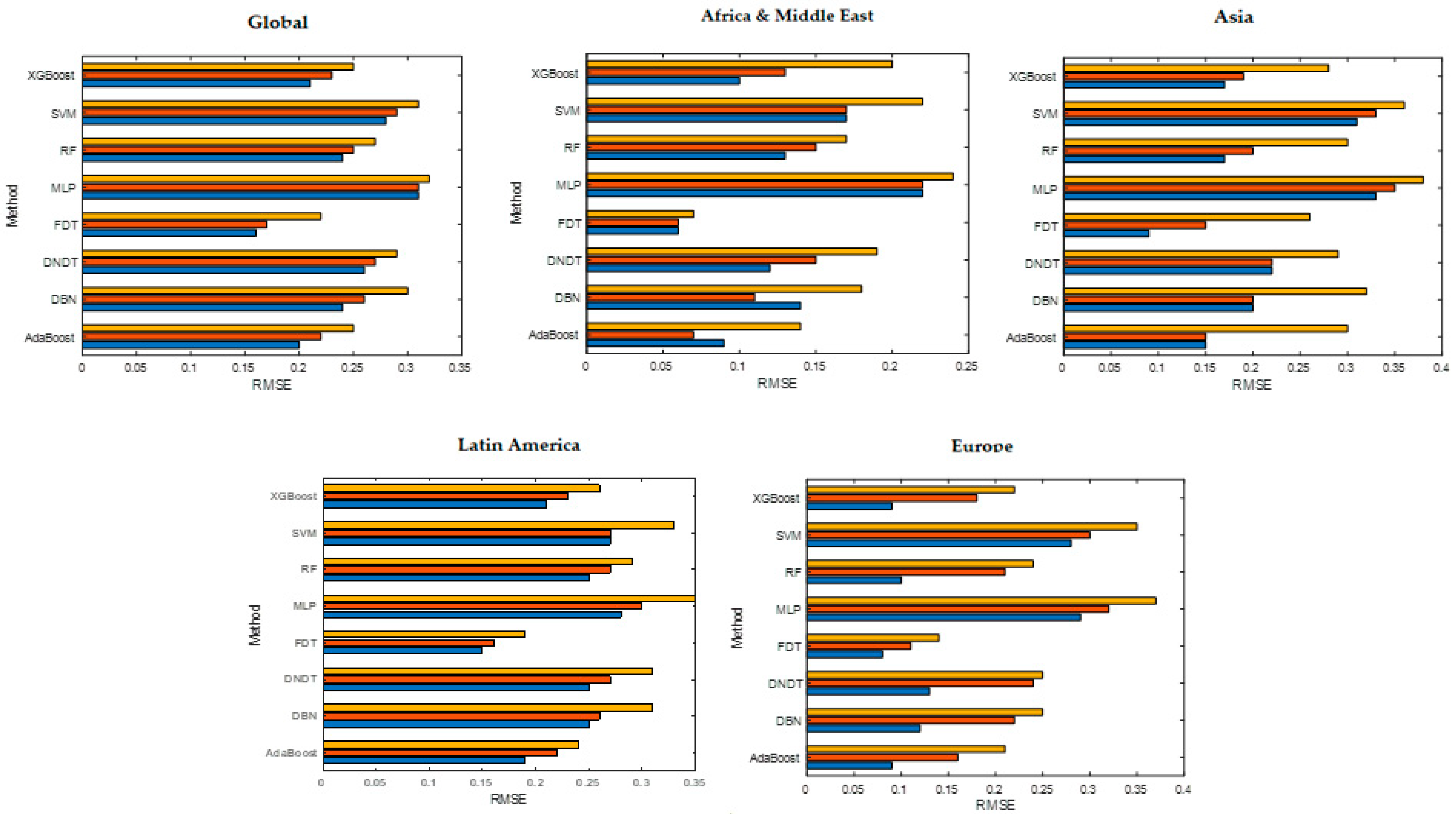
The results of the sensitivity and precision analysis obtained in each stage according to the data subsample (training, validation, and testing) of the global model, Africa, and the Middle East, Asia, Latin America, and Europe, are shown in Table 3 and Table 4, respectively. After observing the results of the sensitivity analysis, the global model shows that variables such as ORR are significant in all the applied methodologies. Another variable that shows the same dynamics is FXR, showing high levels of sensitivity. For their part, the variables that represent credit quality, such as SCFR and SBS, also have high importance according to the results obtained. If we generalize the model in the test sample, the classification level moves in the range 87.67–97.80%, showing the FDT technique with a precision of 97.80% with test data. Finally, the Root Mean Squared Error (RMSE) values (Figure 1) resulting from the methodologies used move in an interval of 0.33–0.22, showing that FDT provides the lowest error (0.22).
The results of the analysis of the sensitivity of the model built with the sample from Africa and the Middle East indicate that the most significant variables are IMFC, M2R, SCFR, and SBS. Regarding the precision results obtained, if we generalize the model in the test sample, the classification level moves in a range of 88.67–100%, with the FDT technique being the one with the highest precision, 100% (testing). Other techniques like AdaBoost and XGBoost show a high level of precision (exceeding 95%). The RMSE values (Figure 1) produced by the methodologies used move in an interval of 0.24–0.07, showing again the FDT technique as the algorithm with the lowest error (0.07).
The variables TRO, FXR, SCFR, and SBS have the greatest impact on the sensitivity analysis of the Asian model. Regarding the precision results, the classification level moves in a range of 8.44–96.82%, showing that FDT presents a precision of 96.82% with test data. In this Asian model, the RMSE values (Figure 1) move in an interval of 0.38–0.26, being again the FDT technique as the algorithm that yields the lowest error (0.26). Regarding the Latin American model, it is observed that the most significant variables are TRO, FXR, SCFR, and SBS. The classification level moves in a range of 87.65–98.85%, showing that FDT obtains the best precision results. In this model, FDT also achieves a lower RMSE. Finally, after examining the results of the sensitivity analysis, the European model shows that the variables with the greatest impact are TDEB, M2R, FXR, SCFR, and SBS. The classification level moves in a range of 86.36–99.76%, with the FDT technique being the one with the highest precision (99.76%). Other techniques such as AdaBoost and XGBoost have also obtained high levels of precision, exceeding 98% in the sample of testing. In this European model, the FDT technique shows the lowest error (0.14).
5.2. Results for Currency Crises
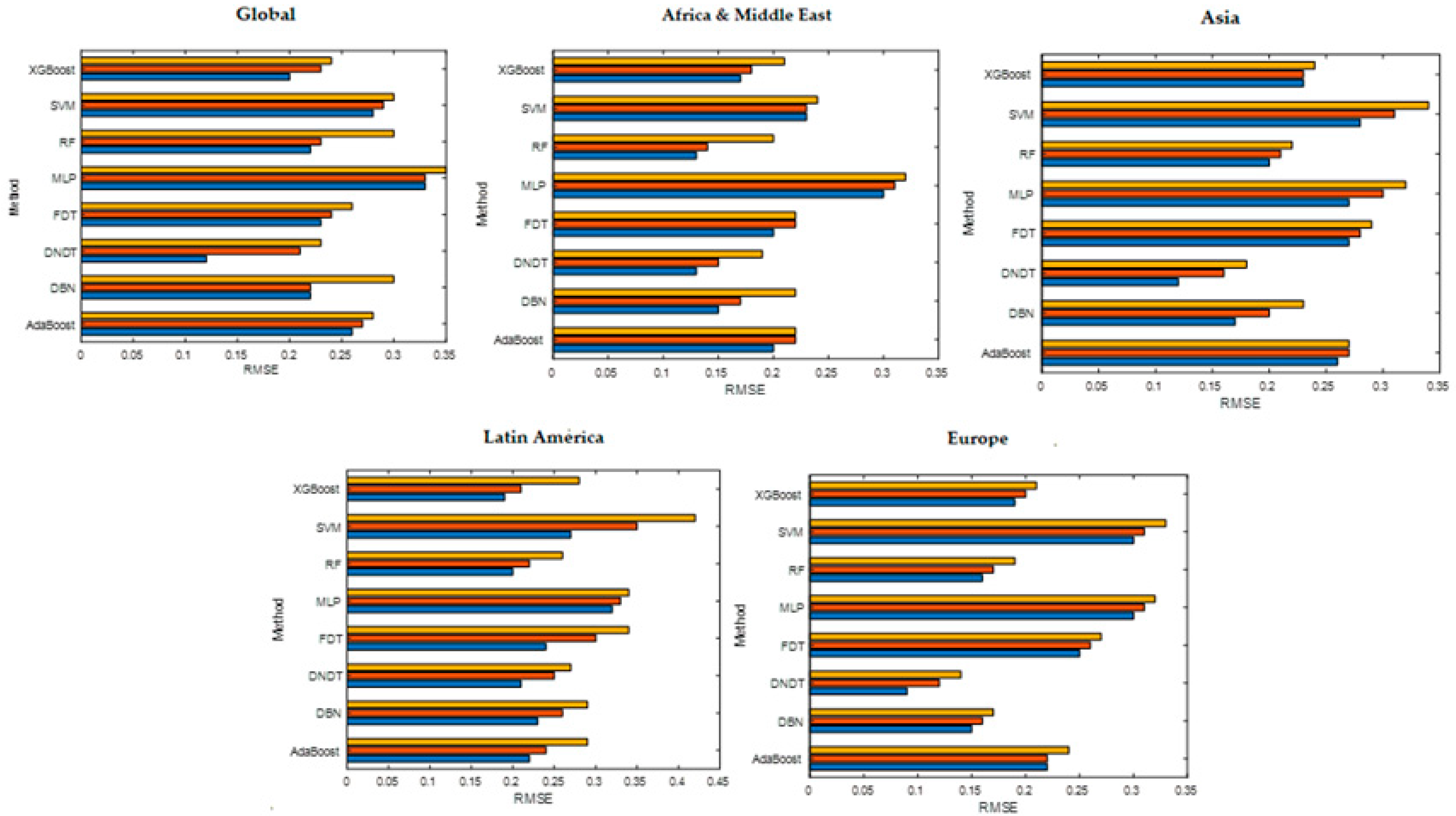
Table 5 and Table 6 detail the results of the sensitivity and precision analysis obtained in each stage according to the data subsample (training, validation, and testing) with the data related to currency crises. In the global model, the most significant variables are M2M, M2R, TRO, FDI, and REER. This shows that a considerable rise in the money supply and foreign investment flows can decide the existence of a global currency crisis. If we generalize the model in the test sample, the classification level moves in a range of 91.83–98.43%, showing that the DNDT technique reaches the highest precision (98.43% with test data). In this global model, the RMSE values (Figure 2) are within the interval 0.35–0.23, showing that the lowest error (0.23) is obtained with FDT.
The Africa and Middle East model shows that M2M, M2R, and FDI are significant with most of the techniques used. Therefore, increases in the money supply and with it, a growth in the proportion of this supply over the country’s foreign exchange reserves, and a low rate of foreign direct investment flows are the best predictors of currency crises in Europe. Regarding the precision of this model, the classification level moves in a range of 92.18–98.24%, showing that the DNDT technique obtains the best fit (precision of 98.24% with test data). Figure 2 details the RMSE values, being the DNDT technique the one with the lowest error (0.19).
The Asian model shows that the variables FXR, TRO, M2R, and CACC show high levels of sensitivity. Therefore, a large increase in the money supply and poor balance of payments and foreign exchange reserve levels appear to be the best currency crisis predictors in Asia. The DNDT technique is the one that offers the highest precision (98.54% with test data). The error range is 0.34–0.18, again being the DNDT technique the one that obtains the lowest (Figure 2). The variables TRO, RGDP, TDEB, and M2R are significant in most of the models built in Latin America. These results indicate that a significant rise in the proportion of the money supply to reserves and a low level of economic growth and trade openness, as well as a high level of public debt, are the main factors in predicting a currency crisis. For its part, the DNDT method is the best prediction technique, with a precision of 96.90% in test data. In this Latin American model, the RMSE values presented by the methods used are located in the interval of 0.34–0.26, with the RF technique being the algorithm with the lowest error (0.26). The results of the sensitivity analysis in the European model show that the variables of M2M, DCRE, FCF, and TDEB are the ones with the greatest impact in most of the applied techniques. These results suggest that an important expansion in the growth of the money supply and high levels of the balance of payments credit and public debt are especially significant in detecting currency crises in Europe. The level of precision is in the range of 92.93–99.07%, with the DNDT technique being the one that reaches a greater success of 99.07% in the testing stage. Figure 2 also details the RMSE values, being the DNDT technique the one with the lowest error (0.14).
5.3. Discussion of Results
The results obtained for the sovereign debt crises forecast reveal a set of robust variables that are reproduced in almost all of the estimated models. Variables of the debt exposure attribute such as TDEB and IMFC mean that the increase in debt levels also causes an increased likelihood of a public debt crisis. These significant variables coincide with the results of the previous works by [3,5], which indicate the great relevance of the debt level on the probability of default. For their part, banking sector variables are significant in previous studies [5], but they have not been validated in our estimates. On the contrary, it has been more common in our models to observe greater significance in variables of the foreign sector attribute such as FXR and M2R, which imply a high accumulation of foreign currency for the payment of the debt of the public institutions of a country. This fact has not been refuted, or at least not with such significance by previous works [7,10]. There are other significant variables such as SCFR and SBS that have not been contrasted either by the prior literature. These variables reflect the fact that a downgrading of the country’s credit rating and an increase in interest payments make it more difficult to access financing and pay the debt, which increases the risk of default due to difficulties in refinancing said debt [3,78]. Lastly, the most sensitive political variables, but with a weaker intensity than those mentioned above, have been: SFI (in the Latin American and Global models) which shows the state’s capacity to carry out public policies, and POLI that shows the country’s level of democracy. In previous literature, only POLI has been identified as significant [3].
The results on sovereign debt default show that models developing with fuzzy C4.5 (FDT) raise the ability to forecast sovereign debt crises, obtaining better ratios of both precision and other selection criteria. Most notably, the global model achieves an accuracy of 97.8%, higher than the 87.1% obtained by [5] employing logistic regression. The same work also reveals the improvement of the precision of their regional models. Along the same lines, it improves the results reported by [3], which had 87% accuracy with regression trees for emerging countries. Likewise, our methodology also improves the prediction capacity of other computational techniques such as neural networks used by [11], with which it obtained 85% accuracy for a sample of emerging countries. Reference [29] achieved 88.6% accuracy with their K-means method for a sample of emerging and developing countries. Even so, other methodologies have shown a consistent predictive capacity throughout the models built, both globally and regionally. These are the case of the AdaBoost, XGBoost, and DNDT techniques, which have shown an average prediction in testing close to 95% correct, making them interesting options to treat the prediction of a sovereign debt crisis. Regarding the level of residuals measured by RMSE, the levels obtained show that the models carried out have a high degree of fit, since the specific statistical literature indicates that those levels below unity present good goodness of fit and that those results less than 0.5 indicate particularly good goodness of fit [79,80]. Therefore, our results show a unique set of variables, in addition to achieving better precision results than the rest of the previous literature.
For their part, the results obtained in the study of currency crises also show a group of explanatory variables that is common in a large part of the estimated models. The FCF variable has been important in most of the models, showing the importance of the evolution of a country’s net investment in increasing the threat of a currency crisis. This result is in contradiction to the findings of [7], in which this variable was not statistically relevant. Continuing with the domestic macroeconomic variables, the variables concerning the money supply (M2M and M2R) have shown high significance, showing that a drastic increase in the money supply hurts the price of the currency. On the other side, the INF variable is not significant, in contrast to works like those of [6,35]. Another variable such as REER has not been refuted as a significant factor either, unlike that shown in the works of [38,45]. Likewise, variables of the foreign sector attribute such as TRO and CACC are shown as more significant variables due to the importance of a country’s international trade performance on price, something that refutes the results of the previous works of [2,36]. In turn, the variables of the banking sector have been relevant in previous investigations [2,6], but they have not obtained a huge significance in our estimates. Regarding the debt variables, the TDEB variable (in connection with the debt accumulation) has been largely significant, indicating that high public debt ratios decrease the currency’s value. Finally, the most important political variables in our models have been: DUR and YEAR (Africa and Asia) that show the state’s capacity to implement public policies, and POLI that shows the level of democracy in the country. These variables have not been pointed as significant in the prior literature [77].
The results on the case of currency crises conclude that the models built with DNDT obtain a forecasting ability close to 100% for currency crises in the regional and global models, with higher levels of accuracy than in other studies. The precision of the global model is 96.38%, but a comparison of this model is complex as it is the first model developed to predict currency crises worldwide. Other studies have obtained lower levels of precision, such as [2], with an accuracy of 84.62% based on the dynamic panel model. In the same way, we have also improved the results obtained by [6], who reached 93.8% accuracy employing neural networks for Turkey. Our methodology is also more powerful in prediction than other computational methods such as the k-nearest neighbor hybrid algorithm and vector support machines (kNN-SVM), which had an accuracy of 97% for a sample of emerging markets [36].
6. Conclusions
The present study developed robust global and regional models to predict international financial crises, specifically those related to sovereign debt and the price of the currency. Similarly, an attempt is made to show the superiority of computational techniques over statistics in terms of the level of precision. An attempt has been made to clarify these issues by overcoming the previous absence of definitive conclusions due to the lack of homogeneity caused by the disparity of methodologies, approaches, available databases, periods, and countries, among other issues.
The results of the study carried out have allowed us to obtain the conclusions that appear below. First, to confirm the existence of differences between the global and regional models, and that the global models can even show a precision capacity similar to the mean of the regional models. To this end, the global sovereign debt prediction models for the studied regions (Africa and the Middle East, Asia, Latin America, and Europe) have obtained an accuracy capacity of 97.80%, 100%, 96.82%, 98%, 85%, and 99.76%, respectively. For its part, this precision relationship for the models built in the study of the currency crisis shows a precision of 98.43%, 98.24%, 98.54%, 96.90%, and 99.07% for the Global sample, Africa and the Middle East, Asia, Latin America, and Europe, respectively. This shows the high level of robustness of the models built concerning previous works.
Second, about the objective that postulated that the application of computational methods could improve the level of precision shown by statistical techniques, our empirical evidence has allowed us to accept it for the analyzed crises, all based on the comparison made between levels of success for test sample data and obtained RMSE values. The best methods for the sovereign debt crisis have been FDT, AdaBoost, XGBoost, and DNDT. While for the prediction of the currency crisis, the best techniques have been DNDT, XGBoost, RF, and DBN.
Regarding the explanatory variables of sovereign debt crises, in the set of estimated models, some variables have appeared as significant continuously. They are the variables related to the exposure to the country’s debt, more specifically TDEB, which shows the importance of a high level of public debt in sovereign default, and IMFC, which indicates the influence of high dependence on credit provided by the IMF as a possible cause of the increased probability of default. On the other hand, the foreign sector variables related to the amount of foreign exchange reserves accumulated by a country, such as FXR and M2R, show the importance of a high level of foreign exchange reserves with which to be able to face international debt payments. Lastly, the SCFR and SBS variables also show continued significance, showing that interest paid and credit rating are important factors when evaluating the possibility of a sovereign default.
The results of the currency crisis prediction models also show that a small group of variables are consistently significant. This is the case of the FCF variable, indicating how a low level of dynamism in net investment in the country can cause a strong drop in the currency’s value. Similarly, the variables that the money supply represents, such as M2M and M2R, indicate that a rise in the money supply in the market makes the currency lose its price. Variables of the foreign sector attribute such as TRO and CACC are also presented as significant variables due to the importance of the commercial opening of a country in the price of its currency. Finally, in the case of naming the most significant political variables in a general way, the variables DUR and YEAR indicate a higher incidence of currency crises in those countries where political regimes are perpetuated, i.e., close to totalitarianism.
6.1. Implications
The above conclusions have important theoretical and practical implications. From a theoretical approach, the models developed can help provide tools for the prevision of sovereign debt and currency crises that are able to avoid international financial crises both at the regional level and as a whole (global), since a high level of robustness in these models concerning previous works. This study is a great contribution to the field of international finance, as the results presented in this work have considerable implications for further decisions, providing tools that help governments and financial markets achieve financial stability. Given the need of countries to obtain financing and establish international relations, our models can help to foresee sovereign debt and currency crises in them, avoiding financial disturbances and imbalances and reducing the possibility of damages in the financial intermediation process. All this implies an improvement in the functioning of financial markets, debt sustainability, the profitability of credit institutions, and the non-banking financial sector, such as investment funds. From a practical point of view, our sovereign debt and currency crisis prediction models can be useful to assess the reputation of a country more accurately. In a globalized world, companies always try to expand into markets outside their own, which makes it vital to enjoying a good image of the country of origin to improve the perception of the goods and services offered. A poor reputation of a country in terms of paying its debt obligations, as well as an unstable currency, can have a negative impact on companies from that country in other markets about seeking financing, suppliers, and partnerships with other companies. Therefore, a better perception of the country’s financial management can improve on the one hand, its position in the financial markets, and, on the other side, the country’s reputation for the benefit of its companies.
6.2. Limitations and Further Research
This investigation has certain limitations, principally the historical data available for emerging economies. As this research was conducted from a globally oriented perspective, it requires a much larger range of information compared to other studies in this field. Furthermore, future studies may delve into other types of political information to deepen their influence both on the financial crises studied and on the impact of the country’s reputation. It would be convenient to relate the influence of the financial crises suffered by a country on exports or tourism, important dimensions in the country’s reputation through modifications of the country strength models, as the main tools for measuring reputation. Likewise, and to increase the generalization of the results in the study of the country’s reputation, further analysis could be included on the impact that the financial strength of a country has on corporate reputation, both in large companies and in those that wish to expand internationally, for instance energy companies.
Machine learning techniques show a great capacity to absorb observations, the use of large data samples being vital to obtain a high level of accuracy. Therefore, it shows a greater margin to achieve better precision ratios and a low level of error. But some of the weaknesses of these computational techniques compared to statistics is their higher computational cost to perform the analyzes, as well as greater difficulty in interpreting some methodologies. Therefore, leaving aside the superiority of machine learning methodologies demonstrated in this study and a multitude of previous works, it is necessary to find new techniques that can mitigate the weaknesses described. An interesting technique to test powerful alternatives for predicting international financial crises, such as their effect on the management of the country’s reputation, would be dynamic systems. This technique has been used in different areas of management, obtaining very satisfactory results in simulations of medium and long-term scenarios [81,82,83,84].
Author Contributions
This study has been designed and performed by all of the authors. D.A and J.I.P. collected the data. D.A., J.I.P. and M.B.S. analyzed the data. The introduction and literature review were written by D.A. and M.A.F.-G. All of the authors wrote the discussion and conclusions. All authors have read and agreed to the published version of the manuscript.
Funding
This research was funded by Cátedra de Economía y Finanzas Sostenibles, Universidad de Málaga, Spain.
Institutional Review Board Statement
Not applicable.
Informed Consent Statement
Not applicable.
Data Availability Statement
Data available on request due to restrictions.
Conflicts of Interest
The authors declare no conflict of interest.
Appendix A

Table A1.
Sovereign debt crisis by country and by year.
| Country | Years | Country | Years | Country | Years |
|---|---|---|---|---|---|
| Albania | 1990 | Finland | Nicaragua | 1980 | |
| Germany | Francia | Niger | 1983 | ||
| Algeria | Gabon | 1986, 2002 | Nigeria | 1983 | |
| Angola | 1988 | Gambia | 1986 | Norway | |
| Argentina | 1982, 2001, 2014 | Georgia | New Zealand | ||
| Armenia | Ghana | Netherlands | |||
| Australia | Grenada | 2004 | Panama | 1983 | |
| Austria | Greece | 2012 | Paraguay | 1982 | |
| Bangladesh | Guinea | 1985 | Perú | 1978 | |
| Belgium | Equatorial Guinea | Poland | 1981 | ||
| Belize | 2007, 2012, 2017 | Guyana | 1982 | Portugal | |
| Bolivia | 1980 | Haiti | United Kingdom | ||
| Brazil | 1983 | Honduras | 1981 | Central African Republic | |
| Brunei | Hong Kong | Czech Republic | |||
| Bulgaria | 1990 | Hungary | Dominican Rep. | 1982, 2003 | |
| Camerún | 1989 | India | Romania | 1982 | |
| Canada | Indonesia | 1999 | Russia | 1998 | |
| Chad | Iran, R.I. | 1992 | Senegal | 1981 | |
| Chile | 1983 | Ireland | Seychelles | 2008 | |
| China, R.P. | Israel | Sierra Leone | 1977 | ||
| Cyprus | 2013 | Italy | Singapore | ||
| Colombia | Jamaica | 1978, 2010 | Syria | ||
| Congo, Rep. | 1986 | Japan | South Africa | 1985 | |
| Congo, D.R. | 1976 | Jordan | 1989 | Sudan | 1979 |
| South Korea | Kazajistan | Sweden | |||
| Ivory Coast | 1984, 2001, 2010 | Kenya | Switzerland | ||
| Costa Rica | 1981 | Kuwait | Thailand | ||
| Croatia | Lebanon | Tanzania | 1984 | ||
| Denmark | Liberia | 1980 | Togo | 1979 | |
| Dominica | 2002 | Libya | Trinidad y Tobago | 1989 | |
| Ecuador | 1982, 1999, 2008 | Madagascar | 1981 | Tunisia | |
| Egypt | 1984 | Malasia | Turkey | 1978 | |
| Slovakia | Malawi | 1982 | Ukraine | 1998, 2015 | |
| Spain | Morocco | 1983 | Uganda | 1981 | |
| United States | Mexico | 1982 | Uruguay | 1983, 2002 | |
| Estonia | Moldavia | 2002 | Venezuela | 1982, 2017 | |
| Ethiopia | Mozambique | 1984 | Vietnam | 1985 | |
| Philippines | 1983 | Namibia | Zambia | 1983 |
Table A2.
Currency crisis by country and by year.
| Country | Years | Country | Years | Country | Years |
|---|---|---|---|---|---|
| Albania | 1997 | Denmark | Jordan | 1989 | |
| Germany | Dominica | Kazajistan | 1999, 2015 | ||
| Algeria | 1988, 1994 | Ecuador | 1982, 1999 | Kenya | 1993 |
| Angola | 1991, 1996, 2015 | Egypt | 1979, 1990, 2016 | Kirguistan | 1997 |
| Argentina | 1975, 1981, 1987, 2002, 2013 | El Salvador | 1986 | Kuwait | |
| Armenia | Eritrea | Laos, R.D.P. | 1972, 1978, 1986, 1997 | ||
| Australia | Slovakia | Lesoto | 1985, 2015 | ||
| Austria | Slovenia | Latvia | 1992 | ||
| Azerbaiyán | 2015 | Spain | 1983 | Lebanon | 1984, 1990 |
| Bangladesh | 1976 | United States | Liberia | ||
| Barbados | Estonia | 1992 | Libya | 2002 | |
| Belgium | Ethiopia | 1993 | Lithuania | 1992 | |
| Belice | Fiji | 1998 | Luxemburgo | ||
| Benín | 1994 | Filipinas | 1983, 1998 | Macedonia | |
| Belarus | 1997, 2009, 2015 | Finland | 1993 | Madagascar | 1984, 1994, 2004 |
| Bolivia | 1973, 1981 | Francia | Malasia | 1998 | |
| Bosnia y Herzegovina | Gabon | 1994 | Malawi | 1994, 2012 | |
| Botsuana | 1984 | Gambia | 1985, 2003 | Maldives | 1975 |
| Brazil | 1976, 1982, 1987, 1992, 1999, 2015 | Georgia | 1992, 1999 | Mali | 1994 |
| Brunei | Ghana | 1978, 1983, 1993, 2000, 2009, 2014 | Morocco | 1981 | |
| Bulgaria | 1996 | Grenada | Mauricio | ||
| Burkina Faso | 1994 | Greece | 1983 | Mauritania | 1993 |
| Burundi | Guatemala | 1986 | Mexico | 1977, 1982, 1995 | |
| Bhutan | Guinea | 1982, 2005 | Moldavia | 1999 | |
| Cape Verde | Equatorial Guinea | 1980, 1994 | Mongolia | 1990, 1997 | |
| Camboya | 1971, 1992 | Guinea-Bissau | 1980, 1994 | Mozambique | 1987, 2015 |
| Cameroon | 1994 | Guyana | 1987 | Myanmar | 1975, 1990, 1996, 2001,2007, 2012 |
| Canada | Haiti | 1992, 2003 | Namibia | 1984, 2015 | |
| Chad | 1994 | Honduras | 1990 | Nepal | 1984, 1992 |
| Chile | 1972, 1982 | Hong Kong | Nicaragua | 1979, 1985, 1990 | |
| China, R.P. | Hungary | Niger | 1994 | ||
| Cyprus | India | Nigeria | 1983, 1989, 1997, 2016 | ||
| Perú | 1976, 1981, 1988 | Sierra Leona | 1983, 1989, 1998 | Trinidad and Tobago | 1986 |
| Poland | Singapore | Tunisia | |||
| Portugal | 1983 | Syria | 1988 | Turkmenistan | 2008 |
| United Kingdom | Sri Lanka | 1978 | Turkey | 1978, 1984, 1991, 1996, 2001 | |
| Central African Republic | 1994 | Swaziland | 1985, 2015 | Ukraine | 1998, 2009, 2014 |
| Czech Republic | South Africa | 1984, 2015 | Uganda | 1980, 1988 | |
| Dominican Rep. | 1985, 1990, 2003 | Sudan | 1981, 1988, 1993, 2012 | Uruguay | 1972, 1983, 1990, 2002 |
| Ruanda | 1991 | South Sudan | 2015 | Uzbekistan | 2000 |
| Romania | 1996 | Sweden | 1993 | Venezuela | 1984, 1989, 1994, 2002, 2010 |
| Russia | 1998, 2014 | Switzerland | Vietnam | 1972, 1981, 1987 | |
| San Cristóbal y Nieves | Surinam | 1990, 1995, 2001, 2016 | Yemen | 1985, 1995 | |
| São Tomé and Príncipe | 1987, 1992, 1997 | Thailand | 1998 | Zambia | 1983, 1989, 1996, 2009, 2015 |
| Senegal | 1994 | Tayikistan | 1999, 2015 | Zimbabue | 1983, 1991, 1998, 2003 |
| Serbia | 2000 | Tanzania | 1985, 1990 | ||
| Seychelles | 2008 | Togo | 1994 |
Table A3.
Frequency of crisis event (number per year).
| Year | Currency Crises | Sovereign Debt Crises |
|---|---|---|
| 1970 | ||
| 1971 | 1 | |
| 1972 | 5 | |
| 1973 | 1 | |
| 1974 | ||
| 1975 | 5 | |
| 1976 | 4 | 1 |
| 1977 | 1 | 1 |
| 1978 | 5 | 3 |
| 1979 | 3 | 2 |
| 1980 | 4 | 3 |
| 1981 | 10 | 6 |
| 1982 | 5 | 9 |
| 1983 | 12 | 9 |
| 1984 | 10 | 4 |
| 1985 | 10 | 3 |
| 1986 | 4 | 3 |
| 1987 | 6 | |
| 1988 | 5 | 1 |
| 1989 | 8 | 3 |
| 1990 | 10 | 2 |
| 1991 | 6 | |
| 1992 | 6 | 1 |
| 1993 | 8 | |
| 1994 | 20 | |
| 1995 | 4 | |
| 1996 | 6 | |
| 1997 | 7 | |
| 1998 | 10 | 2 |
| 1999 | 7 | 2 |
| 2000 | 4 | |
| 2001 | 3 | 2 |
| 2002 | 5 | 4 |
| 2003 | 4 | 1 |
| 2004 | 1 | 1 |
| 2005 | 1 | |
| 2006 | ||
| 2007 | 1 | 1 |
| 2008 | 3 | 2 |
| 2009 | 5 | |
| 2010 | 1 | 2 |
| 2011 | ||
| 2012 | 3 | 2 |
| 2013 | 2 | 1 |
| 2014 | 3 | 1 |
| 2015 | 13 | 1 |
| 2016 | 4 | |
| 2017 | 2 | |
| Total | 236 | 75 |
Table A4.
Results of Logit analysis for sovereign debt crises.
| Variables | Coefficients | Sig. (Wald) | ROC Curve | R2 Nagelkerke | Classification (%) | ||
|---|---|---|---|---|---|---|---|
| Training | Testing | ||||||
| Global | SBS | 0.731 | 0.000 | 0.675 | 0.582 | 79.17 | 77.38 |
| TRO | −0.826 | 0.006 | |||||
| FXR | −0.294 | −0.005 | |||||
| INF | 0.502 | 0.000 | |||||
| Africa and Middle East | IMFC | 1.038 | 0.001 | 0.718 | 0.638 | 85.36 | 81.24 |
| GOVS | 0.592 | 0.007 | |||||
| TDEB | 0.291 | −0.004 | |||||
| SCFR | −0.374 | 0.000 | |||||
| POLI | −0.105 | 0.000 | |||||
| Asia | REER | −1.274 | 0.000 | 0.659 | 0.572 | 81.93 | 78.51 |
| CACC | −0.682 | 0.000 | |||||
| NSAV | −0.719 | 0.007 | |||||
| POLI | −0.073 | 0.000 | |||||
| TDEB | 0.388 | −0.009 | |||||
| Latin America | TRO | −0.737 | 0.000 | 0.725 | 0.653 | 80.28 | 78.14 |
| GOVS | 1.193 | −0.008 | |||||
| SFI | 0.159 | 0.000 | |||||
| IMFC | 0.461 | 0.003 | |||||
| SCLR | −0.153 | 0.005 | |||||
| INF | 0.274 | 0.000 | |||||
| Europe | TDEB | 0.955 | −0.012 | 0.750 | 0.674 | 82.46 | 79.62 |
| M2R | 0.684 | 0.000 | |||||
| GOVS | 1.003 | 0.000 | |||||
| GINT | 0.241 | −0.003 | |||||
| EFEE | −0.639 | 0.000 | |||||
| CDS | 0.146 | 0.000 | |||||
The sample has been divided into 70% for training and 30% for testing.
Table A5.
Results of Logit analysis for currency crises.
| Variables | Coefficients | Sig. (Wald) | ROC Curve | R2 Nagelkerke | Classification (%) | ||
|---|---|---|---|---|---|---|---|
| Training | Testing | ||||||
| Global | M2M | 1.048 | −0.003 | 0.625 | 0.545 | 83.48 | 80.57 |
| M2R | 0.734 | 0.000 | |||||
| POLI | −0.382 | −0.004 | |||||
| REER | −0.285 | 0.013 | |||||
| CACC | −0.419 | 0.000 | |||||
| TRO | −0.118 | 0.000 | |||||
| Africa and Middle East | FDI | −0.892 | 0.000 | 0.727 | 0.621 | 85.94 | 82.26 |
| FCF | −0.537 | −0.008 | |||||
| DCRE | 0.583 | 0.000 | |||||
| CACC | −0.242 | 0.006 | |||||
| Asia | CACC | −1.235 | 0.000 | 0.650 | 0.529 | 86.11 | 83.03 |
| TRO | −0.728 | 0.000 | |||||
| EXP | −0.326 | 0.000 | |||||
| PINV | −0.440 | −0.017 | |||||
| REER | −0.962 | 0.005 | |||||
| DCRE | 0.287 | ||||||
| Latin America | TRO | −0.937 | 0.006 | 0.715 | 0.692 | 84.20 | 81.83 |
| FCF | −0.629 | −0.004 | |||||
| RGDP | −0.249 | 0.000 | |||||
| TDEB | 0.385 | 0.000 | |||||
| DCRE | 0.273 | −0.001 | |||||
| Europe | DCRE | 0.849 | −0.011 | 0.725 | 0.644 | 85.19 | 82.62 |
| M2M | 0.393 | −0.003 | |||||
| RGDP | −0.741 | 0.000 | |||||
| TDEB | 0.361 | 0.004 | |||||
| FCF | −0.104 | 0.000 | |||||
| STD | 0.215 | 0.003 | |||||
The sample has been divided 70% for training and 30% for testing.
References
- Feenstra, R.C.; Taylor, A.M. International Macroeconomics, 2nd ed.; Worth Publishers: New York, NY, USA, 2012. [Google Scholar]
- Candelon, B.; Dumitrescu, E.I.; Hurlin, C. Currency crisis early warning systems: Why they should be Dynamic. Int. J. Forecast. 2014, 30, 1016–1029. [Google Scholar] [CrossRef]
- Savona, R.; Vezzoli, M. Fitting and Forecasting Sovereign Defaults using Multiple Risk Signals. Oxf. Bull. Econ. Stat. 2015, 77, 66–92. [Google Scholar] [CrossRef] [Green Version]
- Ristolainen, K. Predicting Banking Crises with Artificial Neural Networks: The Role of Nonlinearity and Heterogeneity. Scand. J. Econ. 2018, 120, 31–62. [Google Scholar] [CrossRef]
- Dawood, M.; Horsewood, N.; Strobel, F. Predicting Sovereign Debt Crises: An Early Warning System Approach. J. Financ. Stab. 2017, 28, 16–28. [Google Scholar] [CrossRef]
- Sevim, C.; Oztekin, A.; Bali, O.; Gumus, S.; Guresen, E. Developing an early warning system to predict currency crises. Eur. J. Oper. Res. 2014, 237, 1095–1104. [Google Scholar] [CrossRef]
- Boonman, T.M.; Jacobs, J.P.A.M.; Kuper, G.H. Sovereign Debt Crises in Latin America: A Market Pressure Approach. Emerg. Mark. Financ. Trade 2015, 51, S80–S93. [Google Scholar] [CrossRef] [Green Version]
- Alaminos, D.; Fernández, S.M.; García, F.; Fernández, M.A. Data Mining for Municipal Financial Distress Prediction, Advances in Data Mining, Applications and Theoretical Aspects. In Advances in Data Mining. Applications and Theoretical Aspects, Proceedings of the 18th Industrial Conference, ICDM 2018, New York, NY, USA, 11–12 July 2018; Lecture Notes in Computer Science; Springer: Cham, Switzerland, 2018; Volume 10933, pp. 296–308. [Google Scholar] [CrossRef]
- Ari, A.; Cergibozan, R. The Twin Crises: Determinants of Banking and Currency Crises in the Turkish Economy. Emerg. Mark. Financ. Trade 2016, 52, 123–135. [Google Scholar] [CrossRef]
- Dufrénot, G.; Paret, A.G. Sovereign debt in emerging market countries: Not all of them are serial defaulters. Appl. Econ. 2018, 50, 6406–6443. [Google Scholar] [CrossRef]
- Fioramanti, M. Predicting sovereign debt crises using artificial neural networks: A comparative approach. J. Financ. Stab. 2008, 4, 149–164. [Google Scholar] [CrossRef]
- Comelli, F. Comparing Parametric and Non-parametric Early Warning Systems for Currency Crises in Emerging Market Economies; IMF Working Paper, WP/13/134; International Monetary Fund: Washington, DC, USA, 2013. [Google Scholar]
- Caggiano, G.; Calice, P.; Leonida, L. Early warning systems and systemic banking crises in low income countries: A multinomial logit approach. J. Bank. Financ. 2014, 47, 258–269. [Google Scholar] [CrossRef]
- Leiva-Soto, R. The media reputation of Spain during the global financial crisis. Commun. Soc. 2014, 27, 1–20. [Google Scholar]
- Mariutti, F.; Tech, R. Are we talking the Same Language? Challenging Complexity in Country Brand Models. Athens J. Bus. Econ. 2015, 1, 49–62. [Google Scholar] [CrossRef]
- Teodorović, M.; Popesku, J. Country Brand Equity Model: Sustainability Perspective. Marketing 2016, 47, 111–128. [Google Scholar] [CrossRef] [Green Version]
- Papadopoulos, N.; Ibrahim, Y.; De Nisco, A.; Napolitano, M.R. The Role of Country Brandingin Attracting Foreign Investment: Country Characteristics and Country Image. Available online: https://www.francoangeli.it/riviste/Scheda_Rivista.aspx?IDArticolo=61808&Tipo=ArticoloPDF (accessed on 18 March 2020).
- Amador, M.; Phelan, C. Reputation and Sovereign Default; Staff Report 564; Federal Reserve Bank of Minneapolis: Minneapolis, MN, USA, 2018. [Google Scholar]
- Melnyk, T.M.; Varibrusova, A.S. Variable indicators affecting the country’s brand strategy effectiveness and competitiveness in the world. Manag. Sci. Lett. 2019, 9, 1685–1700. [Google Scholar] [CrossRef]
- Vaccaro, G.; Cabrera, F.E.; Pelaez, J.I.; Vargas, G. Comparison matrix geometric index: A qualitative online reputation metric. Appl. Soft Comput. 2020, 96, 106687. [Google Scholar] [CrossRef]
- Charette, F.; d’Astous, A. Country Image Effects in the Era of Protectionism. J. Int. Consum. Mark. 2020, 32, 271–286. [Google Scholar] [CrossRef]
- Lascu, D.; Ahmed, Z.U.; Ahmed, I.; Min, T.H. Dynamics of country image: Evidence from Malaysia. Asia Pac. J. Mark. Logist. 2020, 32, 1675–1697. [Google Scholar] [CrossRef]
- Billio, M.; Casarin, R.; Costola, M.; Pasqualini, A. An entropy-based early warning indicator for systemic risk. J. Int. Financ. Mark. Inst. Money 2016, 45, 42–59. [Google Scholar] [CrossRef] [Green Version]
- Manasse, P.; Roubini, N.; Schimmelpfennig, A. Predicting Sovereign Debt Crises (November 2003); IMF Working Paper, No. 03/221; International Monetary Fund: Washington, DC, USA, 2003; pp. 1–41. [Google Scholar]
- Ciarlone, A.; Trebeschi, G. Designing an early warning system for debt crises. Emerg. Mark. Rev. 2005, 6, 376–395. [Google Scholar] [CrossRef]
- Manasse, P.; Roubini, N. “Rules of thumb” for sovereign debt crises. J. Int. Econ. 2009, 78, 192–205. [Google Scholar] [CrossRef]
- Sarlin, P. Sovereign debt monitor: A visual Self-organizing maps approach. In Proceedings of the 2011 IEEE Symposium on Computational Intelligence for Financial Engineering and Economics (CIFEr), Paris, France, 11–15 April 2011. [Google Scholar]
- Dsoulia, O.; Khan, N.; Kakabadse, N.K.; Skouloudis, A. Mitigating the Davos dilemma: Towards a global self-sustainability index. Int. J. Sustain. Dev. World Ecol. 2018, 25, 81–98. [Google Scholar] [CrossRef] [Green Version]
- Fuertes, A.M.; Kalotychou, E. Optimal design of early warning systems for sovereign debt crises. Int. J. Forecast. 2007, 23, 85–100. [Google Scholar] [CrossRef]
- Arazmuradov, A. Assessing sovereign debt default by efficiency. J. Econ. Asymmetries 2016, 13, 100–113. [Google Scholar] [CrossRef]
- Alaminos, D.; Fernández, S.M.; Neves, P.M.; Santos, J.C. Predicting Sovereign Debt Crises with Fuzzy Decision Trees. J. Sci. Ind. Res. 2019, 78, 733–737. [Google Scholar]
- Lukkezen, J.; Rojas-Romagosa, H. A Stochastic Indicator for Sovereign Debt Sustainability. FinanzArchiv/Public Financ. Anal. 2016, 72, 229–267. [Google Scholar] [CrossRef] [Green Version]
- Lin, C.S.; Khan, H.A.; Chang, R.Y.; Wang, Y.C. A new approach to modeling early warning systems for currency crises: Can a machine-learning fuzzy expert system predict the currency crises effectively? J. Int. Money Financ. 2008, 27, 1098–1121. [Google Scholar] [CrossRef] [Green Version]
- Sarlin, P.; Marghescu, D. Visual predictions of currency crises using self-organizing maps. Intell. Syst. Account. Financ. Manag. 2011, 18, 15–38. [Google Scholar] [CrossRef]
- Chaudhuri, A. Support Vector Machine Model for Currency Crisis Discrimination. arXiv 2014, arXiv:1403.0481. [Google Scholar]
- Ramli, N.A.; Ismail, M.T.; Hooy, H.C. Measuring the accuracy of currency crisis prediction with combined classifiers in designing early warning system. Mach. Learn. 2015, 101, 85–103. [Google Scholar] [CrossRef] [Green Version]
- Mulder, C.; Perrelli, R.; Rocha, M.D. The Role of Bank and Corporate Balance Sheets on Early Warning Systems of Currency Crises—An Empirical Study. Emerg. Mark. Financ. Trade 2016, 52, 1542–1561. [Google Scholar] [CrossRef]
- Boonman, T.M.; Jacobs, J.P.A.M.; Kuper, G.H.; Romero, A. Early Warning Systems for Currency Crises with Real-Time Data. Open Econ. Rev. 2019, 30, 813–835. [Google Scholar] [CrossRef] [Green Version]
- Fratzscher, M. On currency crises and contagion. Int. J. Financ. Econ. 2003, 8, 109–129. [Google Scholar] [CrossRef] [Green Version]
- Yu, L.; Lai, K.K.; Wang, S.Y. Currency Crisis Forecasting with General Regression Neural Networks. Int. J. Inf. Technol. Decis. Mak. 2006, 5, 437–454. [Google Scholar] [CrossRef]
- Yu, L.; Wang, S.; Lai, K.K.; Cong, G. Currency Crisis Forecasting with a Multi-Resolution Neural Network Learning Approach. In Proceedings of the KSS’2007: The Eighth International Symposium on Knowledge and Systems Sciences, Ishikawa, Japan, 5–7 November 2007; Japan Advanced Institute of Science and Technology: Ishikawa, Japan, 2007. [Google Scholar]
- Pham, T.H.A. Are global shocks leading indicators of currency crisis in Vietnam? Res. Int. Bus. Financ. 2017, 42, 605–615. [Google Scholar] [CrossRef] [Green Version]
- Al-Assaf, G. An Early Warning System for Currency Crisis: A Comparative Study for the Case of Jordan and Egypt. Int. J. Econ. Financ. Issues 2017, 7, 43–50. [Google Scholar]
- Karimi, M.; Voia, M.C. Empirics of currency crises: A duration analysis approach. Rev. Financ. Econ. 2019, 37, 428–449. [Google Scholar] [CrossRef]
- Boonman, T.M.; Urbina, A.E.S. Extreme Bounds Analysis in Early Warning Systems for Currency Crises. Open Econ. Rev. 2020, 31, 431–470. [Google Scholar] [CrossRef]
- Berg, B.; Pattillo, C. Predicting currency crises: The indicators approach and an alternative. J. Int. Money Financ. 1999, 18, 561–586. [Google Scholar] [CrossRef]
- Steinberg, D.A.; Koesel, K.J.; Thompson, N.W. Political Regimes and Currency Crises. Econ. Politics 2015, 27, 337–361. [Google Scholar] [CrossRef]
- Alaminos, D.; Becerra-Vicario, R.; Fernández-Gámez, M.A.; Cisneros-Ruiz, A.J. Currency Crises Prediction using Deep Neural Decision Trees. Appl. Sci. 2019, 9, 5227. [Google Scholar] [CrossRef] [Green Version]
- Reinhart, C.; Kaminsky, G.; Lizondo, S. Leading Indicators of Currency Crises; IMF Staff Papers; International Monetary Fund: Washington, DC, USA, 1998; Volume 45, pp. 1–48. [Google Scholar]
- Cumperayot, P.; Kouwenberg, R. Early warning systems for currency crises: A multivariate extreme value approach. J. Int. Money Financ. 2013, 36, 151–171. [Google Scholar] [CrossRef]
- Bucevska, V. Currency Crises in EU Candidate Countries: An Early Warning System Approach. Panoeconomicus 2015, 62, 493–510. [Google Scholar] [CrossRef]
- Núñez de Castro, L.; Von Zuben, F.J. Optimised Training Techniques for Feedforward Neural Networks; Technical Report DCA RT 03/98; Department of Computer Engineering and Industrial Automation, FEEC, UNICAMP: Campinas, Brazil, 1998. [Google Scholar]
- Heidari, E.; Sobati, M.A.; Movahedirad, S. Accurate prediction of nanofluid viscosity using a multilayer perceptron artificial neural network (MLP-ANN). Chemom. Intell. Lab. Syst. 2016, 155, 73–85. [Google Scholar] [CrossRef]
- Lee, D.; Yeo, H. Real-Time Rear-End Collision-Warning System using a Multilayer Perceptron Neural Network. IEEE Trans. Intell. Transp. Syst. 2016, 17, 3087–3097. [Google Scholar] [CrossRef]
- Hearst, M.; Schölkopf, B.; Dumais, S.; Osuna, E.; Platt, J. Trends and controversies–Support vector machines. IEEE Intell. Syst. 1998, 13, 18–28. [Google Scholar] [CrossRef] [Green Version]
- Rawal, B.; Agarwal, R. Improving Accuracy of Classification Based on C4.5 Decision Tree Algorithm Using Big Data Analytics. Computational Intelligence in Data Mining. Adv. Intell. Syst. Comput. 2019, 711, 203–211. [Google Scholar]
- Kingsford, C.; Salzberg, S.L. What are the decision trees? Nat. Biotechnol. 2008, 26, 1011–1013. [Google Scholar] [CrossRef] [PubMed]
- Lee, Y.C.; Chung, P.H.; Shyu, J.Z. Performance evaluation of medical device manufacturers using a hybrid fuzzy MCDM. J. Sci. Ind. Res. 2017, 76, 28–31. [Google Scholar]
- Prashanth, K.D.; Parthiban, P.; Dhanalakshmi, R. Evaluation and ranking of criteria affecting the supplier’s performance of a heavy industry by fuzzy AHP method. J. Sci. Ind. Res. 2018, 77, 268–270. [Google Scholar]
- Alfaro, E.; García, N.; Gámez, M.; Elizondo, D. Bankruptcy forecasting: An empirical comparison of AdaBoost and neural networks. Decis. Support Syst. 2008, 45, 110–122. [Google Scholar] [CrossRef]
- Zhou, L.; Lai, K.K. AdaBoost Models for Corporate Bankruptcy Prediction with Missing Data. Comput. Econ. 2017, 50, 69–94. [Google Scholar] [CrossRef]
- Chen, T.; Guestrin, C. XGBoost: A scalable tree boosting system. arXiv 2016, arXiv:1603.02754. [Google Scholar]
- Chang, Y.C.; Chang, K.H.; Wu, G.J. Application of eXtreme gradient boosting trees in the construction of credit risk assessment models for financial institutions. Appl. Soft Comput. 2018, 73, 914–920. [Google Scholar] [CrossRef]
- Breiman, L. Random forests. Mach. Learn. 2001, 45, 5–32. [Google Scholar] [CrossRef] [Green Version]
- Ho, T.K. Random decision forests. In Proceedings of the International Conference on Document Analysis and Recognition, Montreal, QC, Canada, 14–16 August 1995; IEEE Computer Society: Los Alamitos, CA, USA, 1995. [Google Scholar]
- Raschka, S. Python Machine Learning; Packt Publishing Ltd.: Birmingham, UK, 2015. [Google Scholar]
- Hastie, T.; Tibshirani, R.; Friedman, J. Random Forests. In The Elements of Statistical Learning: Data Mining, Inference, and Prediction, 2nd ed.; Springer: New York, NY, USA, 2009; pp. 587–603. [Google Scholar]
- Bengio, Y. Learning Deep Architectures for Artificial Intelligence. Found. Trends Mach. Learn. 2009, 2, 1–127. [Google Scholar] [CrossRef]
- Yang, Y.; Garcia-Morillo, I.; Hospedales, T.M. Deep Neural Decision Trees. In Proceedings of the 2018 ICML Workshop on Human Interpretability in Machine Learning (WHI 2018), Stockholm, Sweden, 14 July 2018. [Google Scholar]
- Dougherty, J.; Kohavi, R.; Sahami, M. Supervised and unsupervised discretization of continuous features. In Machine Learning: Proceedings of the Twelfth International Conference, Tahoe City, CA, USA, 9–12 July 1995; Morgan Kaufmann Publishers: San Francisco, CA, USA, 1995. [Google Scholar]
- Jang, E.; Gu, S.; Poole, B. Categorical reparameterization with Gumbel-Softmax. arXiv 2016, arXiv:1611.01144. [Google Scholar]
- Delen, D.; Kuzey, C.; Uyar, A. Measuring firm performance using financial ratios: A decision tree approach. Expert Syst. Appl. 2013, 40, 3970–3983. [Google Scholar] [CrossRef]
- Efimov, D.; Sulieman, H. Sobol Sensitivity: A Strategy for Feature Selection. In Mathematics across Contemporary Sciences; AUS-ICMS 2015; Springer Proceedings in Mathematics & Statistics; Springer: Cham, Switzerland, 2015; Volume 190. [Google Scholar]
- Saltelli, A. Making best use of model evaluations to compute sensitivity indices. Comput. Phys. Commun. 2002, 145, 280–297. [Google Scholar] [CrossRef]
- Laeven, L.; Valencia, F. Systemic Banking Crises Revisited; IMF Working Paper, WP/18/206; International Monetary Fund: Washington, DC, USA, 2018. [Google Scholar]
- Kaminsky, G.L. Currency and Banking Crises: The Early Warnings of Distress; International Finance Discussion Papers 629; Board of Governors of the Federal Reserve System: Washington, DC, USA, 1998. [Google Scholar]
- Rother, B. The Determinants of Currency Crises: A Political-Economy Approach Hardcover; Palgrave Macmillan: London, UK, 2009. [Google Scholar]
- Baum, C.F.; Schäfer, D.; Stephan, A. Credit rating agency downgrades and the Eurozone sovereign debt crises. J. Financ. Stab. 2016, 24, 117–131. [Google Scholar] [CrossRef] [Green Version]
- Kalapanidas, E.; Avouris, N.; Craciun, M.; Neagu, D. Machine Learning Algorithms: A Study on Noise Sensitivity. In Proceedings of the First Balkan Conference in Informatics, Thessaloniki, Greece, 21–23 November 2003; pp. 356–365. [Google Scholar]
- Wang, W.; Lu, Y. Analysis of the Mean Absolute Error (MAE) and the Root Mean Square Error (RMSE) in Assessing Rounding Model. In IOP Conference Series: Materials Science and Engineering, Proceedings of the 5th International Conference on Mechanical Engineering, Materials Science and Civil Engineering, Kuala Lumpur, Malaysia, 15–16 December 2017; IOP Publishing: Bristol, UK, 2017; Volume 324, p. 012049. [Google Scholar]
- Di Nardo, M. Developing a Conceptual Framework Model of Industry 4.0 for Industrial Management. Ind. Eng. Manag. Syst. 2020, 19, 551–560. [Google Scholar] [CrossRef]
- Alaminos, D.; León-Gómez, A.; Fernández-Gámez, M.A.; Ferreira, T.S. Next Reaction Method for Solving Dynamic Macroeconomic Models: A Growth Regressions Simulation. J. Sci. Ind. Res. 2020, 79, 277–280. [Google Scholar]
- Di Nardo, M.; Madonna, M.; Murino, T.; Castagna, F. Modelling a Safety Management System Using System Dynamics at the Bhopal Incident. Appl. Sci. 2020, 10, 903. [Google Scholar] [CrossRef] [Green Version]
- Di Nardo, M.; Gallo, M.; Murino, T.; Santillo, L.C. System Dynamics Simulation for Fire and Explosion Risk Analysis in Home Environment. Int. Rev. Model. Simul. 2017, 10, 43–54. [Google Scholar] [CrossRef]
Figure 1.
RMSE values for sovereign debt crises prediction models. Note: training (blue); validation (orange); testing (yellow).
Figure 1.
RMSE values for sovereign debt crises prediction models. Note: training (blue); validation (orange); testing (yellow).

Figure 2.
RMSE values for currency crises prediction models. Note: training (blue); validation (orange); testing (yellow).
Figure 2.
RMSE values for currency crises prediction models. Note: training (blue); validation (orange); testing (yellow).

Table 1.
Definition of the independent variables for the sovereign debt crises.
| Attribute | Abbreviation | Description | Exp. Sign. |
|---|---|---|---|
| Exposure to debt | TDEB | Gross external debt as% of GDP | + |
| IMFC | Loans from the IMF as% of GDP | + | |
| GINT | Global LIR | + | |
| Foreign Sector | FXR | Total reserves (excluding gold) as% of GDP | − |
| TRO | Ratio of exports plus imports to GDP | +/− | |
| EXPG | Annual export growth ratio | − | |
| CACC | Balance of payments account as% of GDP | − | |
| FDI | Foreign direct investment flows as% of GDP | − | |
| Domestic Macroeconomic Factors | RGDP | Annual growth of real GDP | − |
| INF | Rate of change in the consumer price index | + | |
| M2R | Money supply ratio (M2) divided by reserves | + | |
| REER | Deviation of the ratio of the real effective exchange rate of the currency (moving average of the last 5 years) | − | |
| GOVS | Final central government spending as% of GDP | +/− | |
| NSAV | Total savings as% of GDP | − | |
| CON | Sovereign debt crisis event in a country in the same region (t − 1) | + | |
| Banking Sector | DCRE | Domestic credit ratio as% of GDP | +/− |
| BASS | Ratio of bank assets as% of GDP | − | |
| GBL | Net bank claims on the central government | + | |
| Credit Rating Indicators | SCLR | Local currency long-term government bond credit quality scale | +/− |
| SCFR | Scale of the credit quality of the long-term government bond in foreign currency | +/− | |
| SBS | Ratio of interest paid on 10-year public debt bond | + | |
| CDS | Price of public debt bond default insurance | + | |
| Political Factors | FRAG | Political fragmentation score (regional/ethnic tensions) | + |
| POLI | Combined politics score (autocracy score minus democracy score) | +/− | |
| DUR | Durability of the political regime (‘POLI’ control variable) | + | |
| PERS | Number of years since the last radical and abrupt political change. (‘POLI’ control variable) | + | |
| RIR | Score of the magnitude of civil war episodes involving the country (by year) | + | |
| SFI | State fragility index | + | |
| EFEE | Effectiveness of economic policy measured by GDP per capita | − |
Table 2.
Definition of the independent variables for the currency crises.
| Attribute | Abbreviation | Description | Exp. Sign. |
|---|---|---|---|
| Exposure to debt | TDEB | Gross external debt as % of GDP Short-term gross external debt as% of GDP Credit interest rate adjusted for inflation | + |
| STD | Gross external debt as % of GDP Short-term gross external debt as% of GDP Credit interest rate adjusted for inflation | + | |
| RIR | Gross external debt as % of GDP Short-term gross external debt as% of GDP Credit interest rate adjusted for inflation | + | |
| Foreign Sector | FXR | Total reserves (excluding gold) as % of GDP | − |
| TRO | Ratio of exports plus imports to GDP | +/− | |
| IMP | Imports of goods and services in current dollars (USD) | +/− | |
| EXP | Exports of goods and services in current dollars (USD) | − | |
| CACC | Balance of payments account as % of GDP | − | |
| PINV | Net portfolio investment in current dollars (USD) | − | |
| FDI | Foreign direct investment flows as % of GDP | − | |
| Domestic Macroeconomic Factors | RGDP | Annual real GDP in current dollars (USD) | − |
| GDPG | Annual growth of real GDP | − | |
| INF | Rate of change in the consumer price index | + | |
| M2M | Annual growth of money supply (M2) | + | |
| M2R | Money supply ratio (M2) divided by reserves | + | |
| REER | Deviation of the ratio of the real effective exchange rate of the currency (moving average of the last five years) | − | |
| GOVS | Final central government spending as % of GDP | +/− | |
| FCF | Gross fixed capital formation in current dollars (USD) | − | |
| UNE | Total unemployment as % of the total labor force | + | |
| CON | Sovereign debt crisis event in a country in the same region (with a delay of one year) | + | |
| SPEG | Exchange rate regime applied to a currency to keep its value stable against a reserve currency. | + | |
| PEG | Exchange rate regime in which the value of a currency is set against the value of another country’s currency. | + | |
| Banking Sector | DCRE | Domestic credit ratio as % of GDP | +/− |
| LIR | Bank rate that meets the financing needs in the short and medium term | − | |
| DIR | Rate paid by banks for demand, time, or savings deposits | − | |
| Political Factors | POLI | Combined politics score (autocracy score minus democracy score) | − |
| DUR | Durability of the political regime expressed in years (‘POLI’ control variable) | + | |
| PERS | Number of years elapsed since the last radical and abrupt political change (control variable for ‘POLI’) | + | |
| SFI | State frailty index (The higher the score, the greater the risk of frailty) | + | |
| LGOV | Binary variable denoted by 1 if the government has a left ideology, and 0 otherwise | + | |
| ELEC | Binary variable denoted by 1 if it is the year of general elections, and 0 otherwise | + | |
| TURN | Annual rotation of political agents with veto (1—year in which there has been a change of government; 0—otherwise) | + | |
| YEAR | Years in office as president of the national government | + | |
| EFEE | Effectiveness of economic policy measured by GDP per capita | − |
Table 3.
Sensitivity analysis of sovereign debt crises.
| MLP | SVM | FDT | AdaBoost | XGBoost | RF | DBN | DNDT | |||||||||
|---|---|---|---|---|---|---|---|---|---|---|---|---|---|---|---|---|
| Variables | Sensitivity | Variables | Sensitivity | Variables | Sensitivity | Variables | Sensitivity | Variables | Sensitivity | Variables | Sensitivity | Variables | Sensitivity | Variables | Sensitivity | |
| Global | SBS | 0.624 | SBS | 0.482 | TRO | 0.875 | TRO | 0.915 | TRO | 0.767 | TRO | 0.927 | TRO | 0.712 | TRO | 0.755 |
| TRO | 0.619 | FXR | 0.428 | FXR | 0.752 | SCFR | 0.651 | FXR | 0.724 | INF | 0.452 | FXR | 0.561 | FXR | 0.727 | |
| FXR | 0.482 | INF | 0.415 | SCFR | 0.452 | SBS | 0.562 | SFI | 0.406 | SFI | 0.451 | SFI | 0.325 | SFI | 0.652 | |
| SFI | 0.375 | TRO | 0.345 | INF | 0.375 | FXR | 0.519 | SCFR | 0.319 | SCFR | 0.282 | SCFR | 0.321 | |||
| GINT | 0.304 | SFI | 0.375 | |||||||||||||
| Africa & Middle East | IMFC | 1.294 | IMFC | 1.601 | IMFC | 1.370 | IMFC | 0.916 | IMFC | 1.039 | IMFC | 1.023 | IMFC | 1.261 | IMFC | 1.069 |
| POLI | 0.621 | TDEB | 0.612 | TDEB | 0.493 | SCFR | 0.634 | GOVS | 0.526 | TDEB | 0.521 | POLI | 0.542 | TDEB | 0.653 | |
| SCFR | 0.458 | POLI | 0.452 | GOVS | 0.452 | TDEB | 0.451 | TDEB | 0.427 | M2R | 0.378 | GOVS | 0.346 | M2R | 0.631 | |
| M2R | 0.325 | POLI | 0.452 | GOVS | 0.175 | SCFR | 0.237 | SBS | 0.325 | M2R | 0.315 | POLI | 0.329 | |||
| GDPG | 0.321 | SCFR | 0.355 | POLI | 0.194 | GOVS | 0.315 | SCFR | 0.301 | |||||||
| GOVS | 0.305 | GDPG | 0.312 | |||||||||||||
| Asia | CACC | 1.350 | CACC | 1.342 | CACC | 1.157 | CACC | 0.897 | CACC | 1.309 | CACC | 1.215 | CACC | 0.945 | CACC | 1.051 |
| POLI | 0.615 | GDPG | 0.621 | REER | 0.626 | TDEB | 0.436 | REER | 0.571 | SCLR | 0.623 | TDEB | 0.621 | REER | 0.548 | |
| SCLR | 0.521 | M2R | 0.385 | NSAV | 0.502 | NSAV | 0.421 | TDEB | 0.425 | POLI | 0.525 | IMFC | 0.324 | NSAV | 0.451 | |
| NSAV | 0.502 | POLI | 0.317 | TDEB | 0.428 | GINT | 0.325 | FXR | 0.381 | REER | 0.519 | POLI | 0.317 | SCLR | 0.329 | |
| REER | 0.493 | POLI | 0.317 | NSAV | 0.359 | FXR | 0.417 | POLI | 0.308 | |||||||
| GDPG | 0.345 | TDEB | 0.314 | |||||||||||||
| GDPG | 0.312 | |||||||||||||||
| Latin America | TRO | 1.682 | GOVS | 0.910 | TRO | 1.145 | TRO | 1.206 | TRO | 1.243 | TRO | 1.324 | TRO | 0.910 | TRO | 1.231 |
| SFI | 0.956 | TDEB | 0.653 | SFI | 0.625 | SFI | 0.625 | SCLR | 0.652 | GOVS | 0.563 | IMFC | 0.675 | SCLR | 0.634 | |
| SCLR | 0.679 | IMFC | 0.611 | SCLR | 0.452 | IMFC | 0.362 | GOVS | 0.423 | SCLR | 0.458 | SCLR | 0.452 | IMFC | 0.564 | |
| IMFC | 0.454 | TRO | 0.563 | IMFC | 0.427 | GOVS | 0.324 | INF | 0.321 | GINT | 0.328 | SFI | 0.346 | SFI | 0.415 | |
| REER | 0.428 | INF | 0.510 | REER | 0.329 | SFI | 0.315 | SBS | 0.324 | GINT | 0.357 | |||||
| SBS | 0.421 | SFI | 0.462 | GINT | 0.317 | GINT | 0.314 | |||||||||
| SCLR | 0.452 | |||||||||||||||
| REER | 0.323 | |||||||||||||||
| FXR | 0.322 | |||||||||||||||
| Europe | TDEB | 1.428 | TDEB | 1.351 | TDEB | 1.351 | TDEB | 1.452 | TDEB | 1.046 | M2R | 1.014 | M2R | 0.988 | TDEB | 1.152 |
| M2R | 1.145 | M2R | 1.05 | M2R | 1.145 | M2R | 1.231 | M2R | 1.023 | TDEB | 0.965 | TDEB | 0.872 | M2R | 1.061 | |
| GOVS | 0.851 | GINT | 0.452 | GOVS | 0.325 | GINT | 0.514 | GOVS | 0.627 | GDPG | 0.621 | GINT | 0.329 | GOVS | 0.324 | |
| EFEE | 0.462 | EFEE | 0.344 | CACC | 0.347 | CDS | 0.325 | GOVS | 0.384 | GOVS | 0.314 | CACC | 0.314 | |||
| CACC | 0.321 | CDS | 0.322 | GINT | 0.316 | CDS | 0.312 | |||||||||
| GOVS | 0.307 | EFEE | 0.261 | |||||||||||||
Note: Variables with a significance coefficient greater than 0.4 have been chosen.
Table 4.
Accuracy analysis for sovereign debt crises.
| Method | Classification | Global | Africa and Middle East | Asia | Latin America | Europe |
|---|---|---|---|---|---|---|
| MLP | Training | 88.88 | 90.28 | 88.70 | 87.35 | 88.82 |
| Validation | 87.96 | 89.04 | 86.04 | 86.39 | 86.76 | |
| Testing | 87.67 | 88.67 | 85.44 | 87.65 | 86.36 | |
| SVM | Training | 91.09 | 92.80 | 91.30 | 90.06 | 91.12 |
| Validation | 89.41 | 90.98 | 88.41 | 89.72 | 90.67 | |
| Testing | 88.62 | 90.02 | 88.01 | 88.42 | 89.45 | |
| FDT | Training | 98.95 | 100.00 | 100.00 | 99.22 | 100.00 |
| Validation | 98.13 | 100.00 | 98.52 | 99.03 | 99.91 | |
| Testing | 97.80 | 100.00 | 96.82 | 98.95 | 99.76 | |
| AdaBoost | Training | 98.48 | 97.30 | 99.49 | 98.74 | 99.49 |
| Validation | 97.63 | 99.34 | 96.54 | 98.33 | 99.75 | |
| Testing | 96.08 | 98.40 | 95.97 | 97.13 | 99.45 | |
| XGBoost | Training | 97.38 | 96.71 | 97.84 | 97.33 | 99.29 |
| Validation | 96.65 | 96.12 | 96.02 | 97.81 | 99.65 | |
| Testing | 94.42 | 95.26 | 95.43 | 95.44 | 98.19 | |
| RF | Training | 95.46 | 97.95 | 97.25 | 94.88 | 98.92 |
| Validation | 94.68 | 96.25 | 95.89 | 96.28 | 97.80 | |
| Testing | 92.49 | 95.40 | 94.98 | 93.83 | 95.50 | |
| DBN | Training | 95.30 | 95.27 | 96.83 | 94.10 | 98.46 |
| Validation | 93.17 | 94.69 | 94.20 | 95.06 | 96.46 | |
| Testing | 91.71 | 93.70 | 93.95 | 93.76 | 94.02 | |
| DNDT | Training | 96.29 | 97.13 | 97.81 | 94.12 | 99.36 |
| Validation | 94.79 | 96.22 | 96.44 | 95.70 | 98.94 | |
| Testing | 93.43 | 95.30 | 95.20 | 94.23 | 97.58 |
Note: Values expressed in percentage.
Table 5.
Sensitivity analysis of currency crises.
| MLP | SVM | FDT | AdaBoost | XGBoost | RF | DBN | DNDT | |||||||||
|---|---|---|---|---|---|---|---|---|---|---|---|---|---|---|---|---|
| Variables | Sensitivity | Variables | Sensitivity | Variables | Sensitivity | Variables | Sensitivity | Variables | Sensitivity | Variables | Sensitivity | Variables | Sensitivity | Variables | Sensitivity | |
| Global | M2M | 1.315 | TRO | 1.314 | TDEB | 0.872 | M2M | 1.248 | M2R | 1.627 | M2M | 1.248 | M2M | 1.307 | M2M | 1.248 |
| POLI | 0.632 | M2R | 0.981 | M2M | 0.865 | M2R | 1.172 | M2M | 0.827 | RGDP | 0.624 | M2R | 1.152 | M2R | 1.172 | |
| FCF | 0.553 | FCF | 0.814 | M2R | 0.691 | TRO | 0.834 | TRO | 0.725 | REER | 0.524 | TRO | 0.928 | TRO | 0.834 | |
| M2R | 0.523 | TDEB | 0.720 | REER | 0.482 | CACC | 0.624 | FDI | 0.608 | TDEB | 0.501 | TDEB | 0.563 | CACC | 0.624 | |
| TDEB | 0.497 | FDI | 0.689 | FDI | 0.387 | REER | 0.597 | TDEB | 0.472 | TRO | 0.442 | CACC | 0.528 | REER | 0.597 | |
| CACC | 0.437 | POLI | 0.445 | POLI | 0.382 | POLI | 0.382 | REER | 0.425 | POLI | 0.331 | GOVS | 0.520 | TDEB | 0.439 | |
| TRO | 0.435 | GOVS | 0.421 | PINV | 0.335 | FDI | 0.375 | POLI | 0.422 | FDI | 0.324 | REER | 0.517 | POLI | 0.382 | |
| REER | 0.321 | CACC | 0.418 | DCRE | 0.317 | TDEB | 0.318 | FCF | 0.341 | FDI | 0.375 | |||||
| Africa and Middle East | FDI | 1.237 | PINV | 1.428 | FDI | 1.342 | FDI | 1.304 | FDI | 1.12 | M2R | 1.542 | FDI | 1.248 | M2M | 1.732 |
| M2M | 1.226 | FDI | 1.121 | FCF | 0.837 | FCF | 1.283 | TRI | 0.953 | M2M | 1.173 | M2M | 1.228 | FDI | 1.178 | |
| REER | 0.985 | TRO | 0.925 | PINV | 0.628 | M2M | 0.728 | DCRE | 0.871 | FDI | 0.924 | M2R | 0.824 | FCF | 0.785 | |
| FCF | 0.742 | M2M | 0.825 | M2R | 0.62 | TRO | 0.685 | FCF | 0.843 | FCF | 0.824 | DCRE | 0.708 | TRO | 0.748 | |
| M2R | 0.653 | GOVS | 0.756 | TRO | 0.582 | CACC | 0.572 | PINV | 0.781 | CACC | 0.651 | TRO | 0.694 | DCRE | 0.627 | |
| POLI | 0.653 | FCF | 0.647 | POLI | 0.573 | GOVS | 0.561 | M2M | 0.527 | TRO | 0.546 | PINV | 0.675 | M2R | 0.62 | |
| CACC | 0.652 | DCRE | 0.357 | GOVS | 0.561 | POLI | 0.452 | REER | 0.473 | GDPG | 0.379 | CACC | 0.639 | PINV | 0.531 | |
| SFI | 0.582 | POLI | 0.349 | SFI | 0.525 | M2R | 0.34 | POLI | 0.375 | FCF | 0.624 | POLI | 0.493 | |||
| DCRE | 0.538 | CACC | 0.391 | SFI | 0.304 | POLI | 0.315 | CACC | 0.483 | |||||||
| PINV | 0.368 | |||||||||||||||
| Asia | CACC | 1.652 | PINV | 1.562 | M2R | 1.582 | TRO | 1.351 | TRO | 1.067 | TRO | 0.952 | CACC | 1.275 | TRO | 1.351 |
| TRO | 1.223 | TRO | 1.132 | TRO | 1.214 | CACC | 1.181 | DCRE | 0.705 | REER | 0.951 | TRO | 1.274 | CACC | 1.181 | |
| M2R | 0.562 | FXR | 0.924 | EXP | 1.159 | EXP | 0.657 | EXP | 0.621 | FCF | 0.572 | REER | 0.854 | EXP | 0.657 | |
| RIR | 0.523 | FDI | 0.896 | CACC | 0.859 | FXR | 0.634 | FDI | 0.571 | PINV | 0.412 | FXR | 0.634 | FXR | 0.634 | |
| TDEB | 0.452 | POLI | 0.651 | FCF | 0.625 | REER | 0.349 | M2R | 0.481 | RGDP | 0.354 | EXP | 0.512 | REER | 0.349 | |
| EXP | 0.377 | CACC | 0.563 | DCRE | 0.527 | CACC | 0.437 | TDEB | 0.198 | |||||||
| FCF | 0.327 | EXP | 0.547 | REER | 0.349 | RIR | 0.309 | POLI | 0.185 | |||||||
| POLI | 0.324 | GDPG | 0.524 | RGDP | 0.345 | |||||||||||
| Latin America | TRO | 1.314 | GDPG | 1.505 | TRO | 1.528 | TRO | 1.253 | TRO | 1.342 | TRO | 1.321 | TRO | 1.164 | TRO | 1.253 |
| RGDP | 1.256 | TRO | 1.285 | TDEB | 0.899 | RGDP | 1.173 | RGDP | 1.206 | GOVS | 0.851 | RGDP | 1.132 | RGDP | 1.173 | |
| FCF | 0.788 | M2M | 0.895 | GDPG | 0.649 | FCF | 0.593 | FCF | 0.972 | TDEB | 0.715 | TDEB | 0.627 | TDEB | 0.726 | |
| TDEB | 0.687 | DCRE | 0.852 | M2M | 0.618 | TDEB | 0.435 | DCRE | 0.628 | FCF | 0.627 | FCF | 0.505 | FCF | 0.593 | |
| FDI | 0.649 | FCF | 0.683 | POLI | 0.524 | IMP | 0.415 | TDEB | 0.582 | FDI | 0.582 | DCRE | 0.425 | IMP | 0.415 | |
| DCRE | 0.427 | TDEB | 0.652 | DCRE | 0.521 | RIR | 0.317 | FDI | 0.418 | POLI | 0.537 | DCRE | 0.301 | |||
| POLI | 0.354 | FDI | 0.649 | FDI | 0.415 | DCRE | 0.301 | REER | 0.391 | EXP | 0.324 | |||||
| Europe | DCRE | 1.528 | FCF | 1.528 | RGDP | 1.162 | DCRE | 1.518 | M2M | 1.62 | M2M | 1.494 | M2M | 1.529 | DCRE | 1.518 |
| M2M | 1.234 | M2M | 1.293 | M2M | 0.925 | M2M | 1.494 | DCRE | 1.372 | RGDP | 0.952 | DCRE | 1.152 | M2M | 1.494 | |
| FCF | 1.176 | DCRE | 1.184 | DCRE | 0.693 | FCF | 0.843 | TDEB | 0.983 | TDEB | 0.925 | FCF | 0.581 | FCF | 0.843 | |
| PINV | 0.965 | STD | 0.765 | STD | 0.641 | TDEB | 0.648 | FCF | 0.843 | DCRE | 0.527 | TDEB | 0.421 | TDEB | 0.586 | |
| TDEB | 0.326 | TDEB | 0.652 | PINV | 0.581 | STD | 0.415 | PINV | 0.721 | EXP | 0.517 | |||||
| EXP | 0.315 | PINV | 0.541 | GOVS | 0.521 | STD | 0.473 | FCF | 0.355 | |||||||
| SFI | 0.437 | TDEB | 0.458 | GDPG | 0.318 | |||||||||||
Note: Variables with a significance coefficient greater than 0.4 have been chosen.
Table 6.
Accuracy analysis for currency crises.
| Method | Classification | Global | Africa & Middle East | Asia | Latin America | Europe |
|---|---|---|---|---|---|---|
| MLP | Training | 94.84 | 94.44 | 95.06 | 94.12 | 95.43 |
| Validation | 94.27 | 93.91 | 94.52 | 93.37 | 95.10 | |
| Testing | 93.76 | 93.62 | 94.13 | 92.85 | 94.46 | |
| SVM | Training | 93.33 | 93.38 | 93.47 | 93.04 | 93.81 |
| Validation | 92.65 | 92.57 | 93.02 | 92.68 | 93.22 | |
| Testing | 91.83 | 92.18 | 92.61 | 91.95 | 92.93 | |
| FDT | Training | 96.52 | 95.90 | 95.18 | 94.62 | 95.56 |
| Validation | 96.14 | 95.08 | 93.73 | 93.20 | 93.87 | |
| Testing | 95.79 | 94.59 | 93.03 | 92.72 | 93.06 | |
| AdaBoost | Training | 95.95 | 95.25 | 96.17 | 95.08 | 96.86 |
| Validation | 95.34 | 94.57 | 95.64 | 94.21 | 96.42 | |
| Testing | 94.28 | 94.11 | 95.19 | 93.36 | 95.73 | |
| XGBoost | Training | 98.36 | 96.81 | 96.45 | 98.26 | 97.78 |
| Validation | 97.87 | 98.87 | 95.52 | 96.19 | 96.23 | |
| Testing | 97.25 | 95.41 | 95.34 | 95.71 | 96.33 | |
| RF | Training | 96.48 | 98.83 | 98.38 | 98.01 | 98.88 |
| Validation | 94.79 | 97.79 | 97.07 | 97.12 | 97.58 | |
| Testing | 94.01 | 96.52 | 96.17 | 95.93 | 97.01 | |
| DBN | Training | 96.63 | 98.97 | 99.42 | 98.27 | 99.70 |
| Validation | 95.80 | 97.52 | 97.42 | 97.61 | 98.90 | |
| Testing | 94.57 | 96.79 | 96.45 | 96.17 | 98.13 | |
| DNDT | Training | 99.16 | 99.17 | 99.68 | 98.42 | 100.00 |
| Validation | 98.87 | 98.85 | 99.03 | 97.79 | 99.61 | |
| Testing | 98.43 | 98.24 | 98.54 | 96.90 | 99.07 |
Note: Values expressed in percentage.
Publisher’s Note: MDPI stays neutral with regard to jurisdictional claims in published maps and institutional affiliations. |
© 2021 by the authors. Licensee MDPI, Basel, Switzerland. This article is an open access article distributed under the terms and conditions of the Creative Commons Attribution (CC BY) license (https://creativecommons.org/licenses/by/4.0/).
Share and Cite
MDPI and ACS Style
Alaminos, D.; Peláez, J.I.; Salas, M.B.; Fernández-Gámez, M.A. Sovereign Debt and Currency Crises Prediction Models Using Machine Learning Techniques. Symmetry 2021, 13, 652. https://doi.org/10.3390/sym13040652
AMA Style
Alaminos D, Peláez JI, Salas MB, Fernández-Gámez MA. Sovereign Debt and Currency Crises Prediction Models Using Machine Learning Techniques. Symmetry. 2021; 13(4):652. https://doi.org/10.3390/sym13040652
Chicago/Turabian StyleAlaminos, David, José Ignacio Peláez, M. Belén Salas, and Manuel A. Fernández-Gámez. 2021. "Sovereign Debt and Currency Crises Prediction Models Using Machine Learning Techniques" Symmetry 13, no. 4: 652. https://doi.org/10.3390/sym13040652
Note that from the first issue of 2016, this journal uses article numbers instead of page numbers. See further details here.