CFD Simulations of Radioembolization: A Proof-of-Concept Study on the Impact of the Hepatic Artery Tree Truncation

Abstract

Radioembolization (RE) is a treatment for patients with liver cancer, one of the leading cause of cancer-related deaths worldwide. RE consists of the transcatheter intraarterial infusion of radioactive microspheres, which are injected at the hepatic artery level and are transported in the bloodstream, aiming to target tumors and spare healthy liver parenchyma. In paving the way towards a computer platform that allows for a treatment planning based on computational fluid dynamics (CFD) simulations, the current simulation (model preprocess, model solving, model postprocess) times (of the order of days) make the CFD-based assessment non-viable. One of the approaches to reduce the simulation time includes the reduction in size of the simulated truncated hepatic artery. In this study, we analyze for three patient-specific hepatic arteries the impact of reducing the geometry of the hepatic artery on the simulation time. Results show that geometries can be efficiently shortened without impacting greatly on the microsphere distribution.

1. Introduction

Liver cancer is one of the leading types of cancer in incidence and mortality rates worldwide [1]. Radioembolization (RE) is a safe and effective intraarterial targeted therapy for unresectable primary and secondary liver tumors and it consists in the microcatheter-based infusion of yttrium-90 (Y-90) radiolabeled microspheres that are transported in the bloodstream until they get lodged in the tumoral tissue, where they deliver high tumoricidal doses of radiation to cancer cells, while ideally sparing healthy liver parenchyma [2].

In the last decade, a number of studies have been published on the computational fluid dynamics-based (CFD) simulation of the hepatic artery hemodynamics and microsphere transport during RE [3]. Some studies have focused on the type of microcatheter (e.g., standard end-hole microcatheter, antireflux catheter, angled-tip microcatheter) [4,5,6], and others have focused on the influence of various treatment and patient parameters (e.g., injection velocity, microcatheter location, hepatic artery geometry, etc.) on the microsphere distribution [7,8,9]. The ultimate goal of these studies is to provide the multidisciplinary team (interventional radiologists, hepatologists, nuclear oncologists, nuclear medicine physicians, etc.) that plans the treatment with additional information that can be of interest when planning the treatment. Moreover, CFD-based computer platforms have been presented in the literature for RE planning, such as the Computational Medical Management Program, by which the optimal temporal and spatial points for microsphere infusion are determined [10] or CFDose, a simulation-based tool to calculate the patient-specific dosimetry to be infused to the patient [11]. However, the former can be used with a smart microcatheter (not commercially available yet) whose tip can be placed at a specified location within the infusion cross-sectional plane and a microsphere delivery system (not commercially available yet) that infuses at a specified temporal point in the cardiac cycle.

These simulation-based tools must be fast enough in providing results to be of use in the clinical setting. The phenomena involving the microsphere–hemodynamics have been proved to be dependent on local effects near the microcatheter tip, therefore three-dimensional (3D) and transient models are needed [3]. One could use CFD simulations or fluid–structure interaction (FSI) simulations, which consider the interaction between the fluid and the (rigid or deformable) solid. However, FSI simulations are far more expensive computationally than CFD simulations. A study by Childress et al. [12] showed that using CFD simulations instead of FSI simulations resulted in an important simulation-time reduction (3.5 days vs. 11–14 h [in a 10-processor 6-core 40-GB-RAM 3.33-GHz CPU]), with minor influence in the results, so CFD simulations could suffice.

One approach to reduce current CFD simulations’ computational time would be the reduction of the size of the geometry where the CFD simulation is carried out. This geometry simplification should not result in marked differences in the calculated segment-to-segment microsphere distribution. Therefore, the hypothesis behind this study is that simulation times can be reduced considerably if the arterial geometry is effectively shortened, whether downstream or upstream (or both) from the microcatheter-tip location, obtaining a segment-to-segment microsphere distribution similar to that of the baseline geometry simulation. To do so, a geometry-reduction strategy is developed with one patient-specific case and this strategy is applied to two other patient-specific cases to assess the impact of the reduction on the simulation results, in terms of downstream microsphere distribution, and simulation times were analyzed.

2. Materials and Methods

In this section, we first introduce the three patients that are modeled in this study (one for developing the geometry-reduction strategy and two additional cases where the strategy is applied and assessed). Second, we show the baseline and simplified versions of the three 3D patient-specific hepatic artery geometries used in this study. For the first geometry, Patient 1, we conducted a step-by-step upstream and downstream simplification process to analyze to what extent each simplification influences the segment-to-segment microsphere distribution. Patient 2 and Patient 3′s hepatic arteries were later simplified accordingly. Finally, the CFD model is presented.

2.1. Patients: Hepatic State and Radioembolization

This study was done using the patient-specific geometry of three patients: hereafter (Patient 1, Patient 2, and Patient 3,

Table 1. Patient 1 liver mass volumes and blood flow rates per segment.

Segment	Healthy Tissue Volume (mL)	Tumor Volume (mL)	Volumetric Flow Rate (mL/min)
S1	-	-	-
S2	241	-	24.1
S3	96	-	9.6
S4a	24	-	2.4
S4b	48	-	4.8
S5	330	-	33
S6	183	-	18.3
S7	228	-	22.8
S8	340	68	68
Total	1490	68	183

,

Table 2. Patient 2 liver mass volumes and blood flow rates per segment.

Segment	Healthy Tissue Volume (mL)	Tumor Volume (mL)	Volumetric Flow Rate (mL/min)
S1	-	-	-
S2	157.8	-	15.8
S3	157.4	-	15.7
S4	309.4	-	30.9
S5	151.7	-	15.2
S6	193.1	-	19.3
S7	155.3	-	15.5
S8	385.4	77.1	77.1
Total	1510	77.1	189.5

and

Table 3. Patient 3 liver mass volumes and blood flow rates per segment.

Segment	Healthy Tissue Volume (mL)	Tumor Volume (mL)	Volumetric Flow Rate (mL/min)
S1	62	-	6.2
S2	128	-	12.8
S3	181	-	18.1
S4a	73	-	7.3
S4b	11	-	1.1
S5	124	-	12.4
S6	169	-	16.9
S7	373	-	37.3
S8	204	39.8	40.3
Total	1325	39.8	152.4

). Regarding the geometries, these were reconstructed with MeVis (MeVis Medical Solutions AG, Bremen, Germany). Regarding the liver segment volumes, with segments defined as proposed by Couinaud [13], these were either obtained from the report provided by MeVis (Patients 1 and 3, Table 1 and Table 3) or they were taken from the literature to be physiologically realistic (total volume according to reference [14] and fractional segmental volume according to reference [15]) (Patient 2, Table 2). As for the cancer scenarios, the same fictional cancer scenario was posited in the three patients. The scenario consists of a hepatocellular carcinoma (HCC) in segment 8. The tumor volume is equal to 20% of the healthy tissue volume of segment 8.

The perfusion model developed by Aramburu et al. was used to determine the segmental arterial blood flow rates [16]. A normal/healthy tissue perfusion of k₁ = 0.1 mL min⁻¹ mL⁻¹ was adopted for all segments, with a tumor tissue perfusion of k₂ = 0.5 mL min⁻¹ mL⁻¹ [17,18]. In this model, the average blood flow rate flowing towards a segment s, i.e., $q_s$, is calculated with Equation (1):

$$q_s=V_{0,s}{k}_1+V_{\mathrm{c},s}{k}_2,$$

(1)

where $q_s$ is the volumetric flow rate to segment s (with s from segment 1 [S1] to segment 8 [S8]), $V_{0,s}$ is the volume of healthy tissue in segment s, $V_{\mathrm{c},s}$ is the volume of the tumor tissue in segment s, $k_1$ is the healthy tissue arterial perfusion, and $k_2$ is the tumor tissue arterial perfusion. Table 1, Table 2 and Table 3 collect the liver volumes and flow rates of each patient analyzed per segment.

The RE treatment was computer-simulated with Y-90 resin SIR-Spheres^® (Sirtex Medical Limited, Australia). The activity to be delivered was calculated with the body surface area method [19], assuming a 1.76 m 74 kg male in all cases. According to this method, 1.7 GBq must be administered in the analyzed cases, that is, approximately 34 million microspheres.

The infusion device modeled was a 2.7 F end-hole microcatheter with inner and outer diameters of D_in = 0.65 mm and D_out = 0.9 mm, respectively, modeling a Progreat^® microcatheter (Terumo, Tokyo, Japan). A selective catheter location was modeled and located before the first branch that irrigates segment 8, approximately in the initial 1/3 of the branch. The tip of the microcatheter was radially centered in the lumen of the artery. An additional microcatheter location was assumed for Patient 2, explained later.

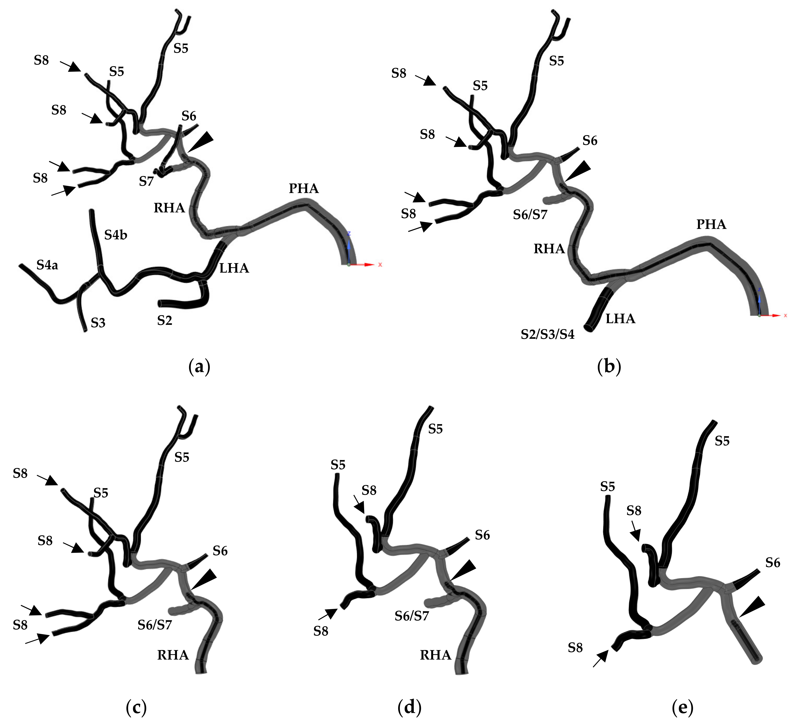
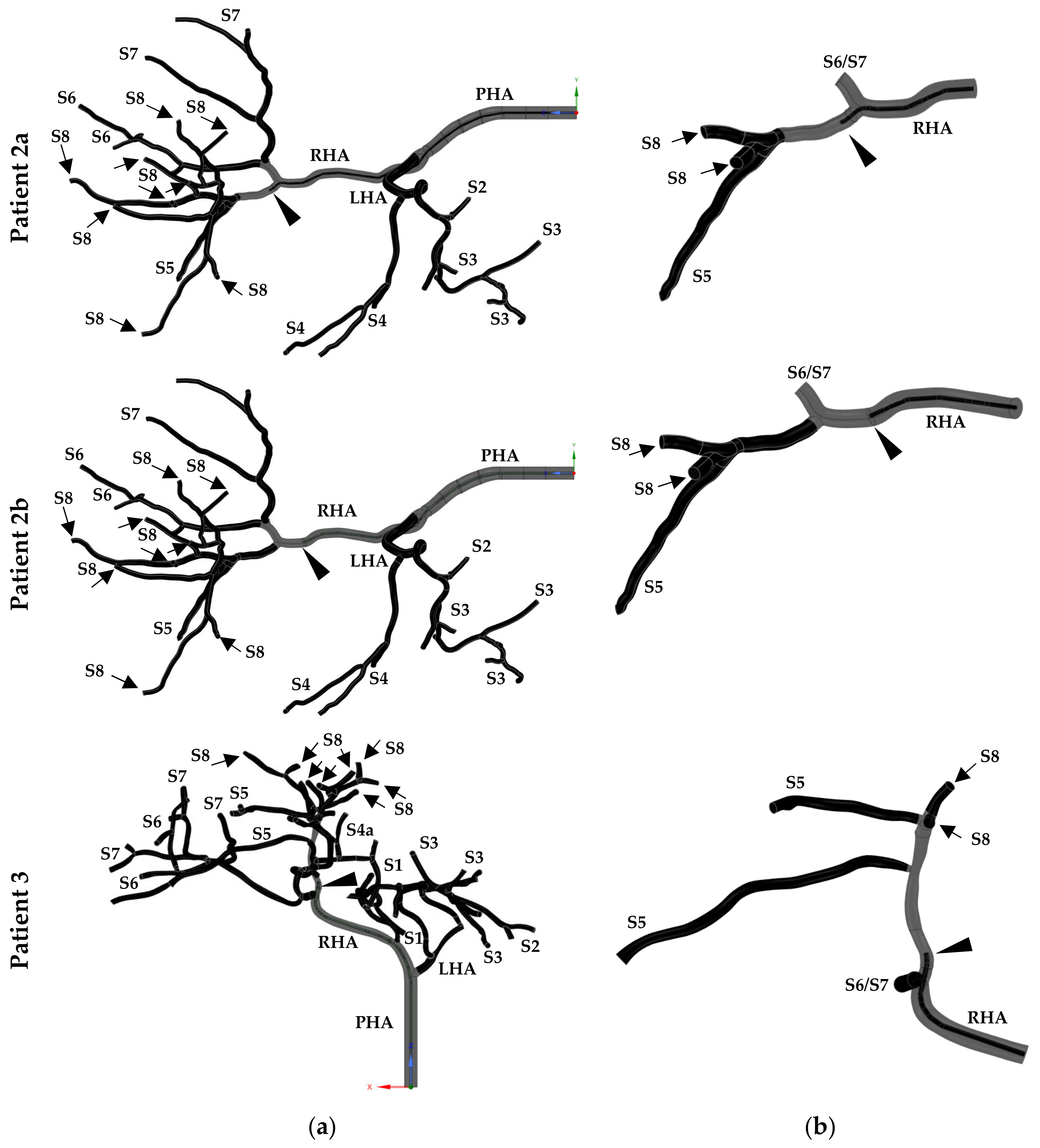
2.2. Baseline and Simplified Hepatic Artery Geometries

As previously said, the geometry of Patient 1′s hepatic artery was modified step by step, with the aim of generating a rule that ensures that the segment-to-segment microsphere distributions calculated from the simulations with the baseline and simplified geometries are similar. Once the simplification with the desired characteristics (i.e., minor impact on segment-to-segment microsphere distribution) were obtained, hepatic arteries for Patient 2 and Patient 3 were likewise simplified. For Patient 1 (Patient 1-Baseline), four simplifications were made to the baseline geometry. Figure 1 shows the geometries obtained from the simplifications. The arrowhead illustrates the microcatheter-tip position in each case, arrows indicate the branches feeding the tumor-bearing segment 8, and labels S1–S8 indicate the segment(s) that each outlet irrigate(s). First, the upstream branches were removed, giving as a result two simplifications. The first one consists of a simplified geometry where the branches irrigating the segments with no tumors are truncated (Patient 1-Reduc1, see Figure 1b). In the second (upstream) simplification, in addition to the simplifications made in the first (upstream) simplification, all the upstream branches that are farther than 3 cm from the microcatheter-tip are removed (Patient 1-Reduc2, see Figure 1c). Then, the downstream branches were simplified, truncating at locations where the bifurcation gives rise to two daughter vessels that irrigate the same segment (Patient 1-Truncated-3cm, see Figure 1d). Finally, the geometry has been truncated before the first bifurcation, adding a branch in the perpendicular direction to the inlet boundary, with the same diameter and a length of 1 cm (Patient 1-Reduc3, see Figure 1e). This final simplification is for obtaining a fully developed-like flow on original inlet section.

The criterion that we are going to establish to deem a simplification as valid is a maximum of 10 percent points of difference at a given segment between the segment-to-segment microsphere distributions of the simulations of the baseline and simplified geometries. In the clinical application of these simulations, we are interested in predicting the segment-to-segment microsphere distribution for a potential improvement in the treatment planning, so the validity criterion of the simplification is based on these results. Qualitative assessment of velocity contours and vectors is used to analyze if the geometry reduction-related changes in blood-flow patterns are excessive.

After analyzing (quantitatively) the segment-to-segment microsphere distributions and (qualitatively) the flow characteristics (velocity magnitude contours and vectors) near the microcatheter tip for the truncated geometries of Patient 1, the selected truncated geometry is the geometry shown in Figure 1d, that is, the geometry with the following characteristics: all the upstream branches that are farther than 3 cm from the microcatheter tip are truncated and all the downstream branches that, after a bifurcation feed, had the same segment truncated as well. This is because this geometry is the shortest geometry that fulfills the imposed 10 percent point difference limit in microspheres segment-to-segment distribution for a given segment. The same rule followed to generate Patient 1-Truncated-3cm was used to define the truncated geometries of Patient 2 (Patient 2a-Truncated-3cm) and Patient 3 (Patient 3-Truncated-3cm), shown in Figure 2.

The three cases reported have a bifurcation between the microcatheter tip and the 3-cm upstream truncation. A second microcatheter-tip location was chosen for Patient 2, to study an extra case that has no bifurcation in this inlet-to-microcatheter-tip zone, hereafter Patient 2b, being Patient 2a the case with the original microcatheter-tip location (see Figure 2 top and middle panels).

2.3. Preprocessing

2.3.1. Spatial Domain Discretization

All the geometries described in the Section 2.2 were discretized following the same procedure and Fluent Meshing 2020R1 (ANSYS Inc., Canonsburg, PA, USA) software package. The type of elements used was poly-hexahedral. The general settings for generating the mesh include a maximum element size of 0.2 mm, a minimum element size of 0.02 mm and a growth rate of 1.1. A local body sizing was also used for the microcatheter with an element size of 0.05 mm. Finally, inflation layers were used in all the walls to capture the boundary layer in sufficient detail. This refinement has 4 layers, the first layer with 0.01 mm and increases with a growth rate of 1.1.

Table 4. Element quantity comparison (in millions).

Patient	Baseline Geometry	Truncated Geometry
Patient 1	3	0.8
Patient 2a	5	0.8
Patient 2b	4.7	0.95
Patient 3	3.8	0.6

shows the quantity of elements of the baseline and truncated geometries.

2.3.2. Mathematical Modeling

In modeling the RE treatment, the hemodynamics and the Y-90 resin microsphere transport were modeled. The mathematical model used in this work is the one presented in Aramburu et al. [8]. Regarding the hemodynamics, blood was assumed an isothermal, incompressible, non-Newtonian fluid flowing in laminar regime. The governing equations are the conservation of mass (Equation (2)) and the conservation of the linear momentum (per unit blood volume) (Equation (3)) read:

$$\nabla ·u=0,$$

(2)

$$\rho \left(\frac{\partial u}{\partial t}+\nabla ·\left(uu\right)\right)=-\nabla p+\nabla ·\mathsf{\tau }+F,$$

(3)

where $u$ is the fluid velocity vector, $\rho$ is the fluid density (1050 kg/m³ [20]), $p$ is the fluid pressure, $F$ is the body force per unit volume, and $\mathsf{\tau }$ is the stress tensor, which is defined as in Equation (4) for blood:

$$\mathsf{\tau }={\mu }_{\mathrm{app}}\left(\dot{\gamma }\right)[\nabla u+{\left(\nabla u\right)}^{\mathrm{T}}],$$

(4)

where ${\mu }_{\mathrm{app}}\left(\dot{\gamma }\right)$ is the apparent blood viscosity, which depends on the shear rate ($\dot{\gamma }$) as indicated in Equations (5) and (6) [7]:

$$\mu \left(\dot{\gamma }\right)=\max \left\{{\mu }_0,{\left(\sqrt{{\mu }_{\infty }}+\frac{\sqrt{{\mathsf{\tau }}_0}}{\sqrt{\mathsf{\lambda }}+\sqrt{\dot{\gamma }}}\right)}^2\right\},$$

(5)

$$\dot{\gamma }=\sqrt{\nabla u[\nabla u+{\left(\nabla u\right)}^{\mathrm{T}}]},$$

(6)

where ${\mu }_0$ = 0.00309 Pa·s, ${\mu }_{\infty }$ = 0.002654 Pa·s, ${\tau }_0$ = 0.004360 Pa, and $\mathsf{\lambda }$ = 0.02181 s⁻¹ are the minimum viscosity, asymptotic viscosity, the apparent yield stress, and the shear stress modifier, respectively [7,12,21,22,23,24,25].

Microspheres were modeled as 32 μm 1600 kg/m³ spheres. The Discrete Phase Model of Fluent 2020R1 (ANSYS^® Inc.) was used to calculate the microsphere trajectory in a Lagrangian reference frame, using a two-way blood–microsphere interaction coupling, and considering no interaction between microspheres. Microsphere motion is governed by the Newton’s Second Law of Motion, in which the virtual mass force, pressure gradient force, gravitational force, and drag forces are considered as in reference [8]. This governing equation expressed per unit microsphere mass reads (Equation (7)):

$$\frac{\mathrm{d}{u}_{\mathrm{p}}}{\mathrm{d}t}=f_{\mathrm{V}}+f_{\mathrm{P}}+f_{\mathrm{G}}+f_{\mathrm{D}},$$

(7)

where $u_{\mathrm{p}}$ is the velocity of the particle (i.e., the microsphere), and $f_{\mathrm{V}}$, $f_{\mathrm{P}}$, $f_{\mathrm{G}}$, and $f_{\mathrm{D}}$, are the virtual mass (Equation (8)), pressure gradient (Equation (9)), gravitational (Equation (10)), and drag (Equation (11)) forces, respectively:

$$f_{\mathrm{V}}=C_{\mathrm{V}}\frac{\rho }{{\rho }_{\mathrm{p}}}\left[\left(u_{\mathrm{p}}·\nabla \right)u-\frac{\mathrm{d}{u}_{\mathrm{p}}}{\mathrm{d}t}\right],$$

(8)

where $C_{\mathrm{V}}$ is the virtual mass force coefficient and ${\rho }_{\mathrm{p}}$ is the particle (i.e., microsphere) density,

$$f_{\mathrm{P}}=\frac{\rho }{{\rho }_{\mathrm{p}}}\left(u_{\mathrm{p}}·\nabla \right)u,$$

(9)

$$f_{\mathrm{G}}=\frac{{\rho }_{\mathrm{p}}-\rho }{{\rho }_{\mathrm{p}}}g,$$

(10)

where g is the vector of the acceleration of gravity, 9.81 m/s² in magnitude and considering patient’s recumbent position during injection,

$$f_{\mathrm{D}}=\frac{18{\mu }_{\mathrm{app}}}{{\rho }_{\mathrm{p}}{d}_{\mathrm{p}}^2}\frac{C_{\mathrm{D}}{\mathrm{Re}}_{\mathrm{p}}}{24}\left(u-u_{\mathrm{p}}\right),$$

(11)

where $d_{\mathrm{p}}$ is the particle (i.e., microsphere) diameter, $C_{\mathrm{D}}$ is the drag coefficient, and ${\mathrm{Re}}_{\mathrm{p}}$ is the particle (i.e., microsphere) Reynolds number (Equation (12)):

$${\mathrm{Re}}_{\mathrm{p}}=\frac{\rho d_{\mathrm{p}}\left|u_{\mathrm{p}}-u\right|}{{\mu }_{\mathrm{app}}}.$$

(12)

2.3.3. Boundary Conditions

The boundary conditions prescribed are similar to those presented in Aramburu et al. [16], i.e., inflows at the inlets and inflow fractions (percentages of the total inflow) at the outlets. This model considers the arterial blood flow need of each segment and distributes the blood in the computational domain according to these needs. Regarding the inlet section of the artery, an inflow waveform was prescribed. Figure 3 shows the six periodic (period = 1 s) waveforms used, two per patient. To calculate the mean values of the waveforms, the perfusion model developed by Aramburu et al. [16] and applied to these three patients in Section 2.1 was used (see row “Total” in Table 1, Table 2 and Table 3) for the baseline geometries. For the truncated geometries, the segments irrigated from the inlet section were considered. These waveforms were translated into uniform velocities at the inlet section. At the inlet section of the microcatheter, a uniform constant velocity equal to the systolic peak velocity was prescribed. With regard to the outlet sections, the flow fractions were prescribed, i.e., the percentage of the total inflow flowing through each outlet. The flow split was defined as explained in Aramburu et al. [16], where the flow fraction at an outlet depends on the flow toward the segment that the outlet is feeding (calculated with Equation (1)) and the level of generation the outlet is located at. For example, if a segment is irrigated by a tree consisting of an artery that bifurcates into branch 1 and branch 2, which bifurcates into branch 3, and branch 4 and outlets are at branches 1, 3, and 4, then 50% of the blood flow will be provided by the outlet at branch 1, and 25% will be provided by each outlet at branches 3 and 4. Walls were assumed as rigid, impermeable, with no relative velocity between the wall velocity and fluid velocity (no-slip condition) and the impact between walls and microspheres was assumed as elastic.

For the mass flow rate of microspheres to be injected, it was assumed that all the microspheres were diluted in a 5-mL vial. Microspheres were assumed to be injected with the initial concentration in the vial. Hence, the prescribed microsphere mass flow rates for Patient 1, Patient 2, and Patient 3 were 2.040 × 10⁻⁵ kg/s, 2.119 × 10⁻⁵ kg/s, and 2.096 × 10⁻⁵ kg/s, respectively.

2.4. Solver Settings

The governing equations of hemodynamics and microsphere transport were solved numerically using the finite volume method-based Fluent 2020R1 (ANSYS Inc.). The pressure and velocity were solved in a segregated way using the SIMPLE scheme for pressure–velocity coupling. Gradients were computed using a least squares cell-based algorithm, and the pressure and momentum interpolations were done with a second order algorithm. Finally, the transient formulation was defined as a second order implicit, with a fixed time step of 2 × 10⁻³ s. The maximum iterations per time step was limited to 80.

Regarding the convergence criteria used, minimum residuals of 1 × 10⁻⁵ were fixed for continuity and the three components of the velocity.

Regarding the number of cardiac cycles simulated, RE was simulated as follows: a first cardiac cycle was simulated (t = −1 s to t = 0 s) to eliminate the influence of the initial value (i.e., the convergence cycle). Then the actual simulation began. Microspheres were injected during the first cardiac cycle (t = 0 s to t = 1 s) (i.e., the injection cycle). Two extra cardiac cycles were simulated without injecting more microspheres (t = 1 s to t = 3 s) (i.e., extra cycle 1 and extra cycle 2). These two extra cardiac cycles are simulated to ensure that the fraction of exiting microspheres reach a steady value over time. Therefore, four cardiac cycles are simulated per simulation. With these results, we could extrapolate the final distribution of all the microsphere of the vial, assuming that the microsphere distribution will remain unchanged throughout the treatment. This model provides a prediction of the outlet-to-outlet microsphere distribution (of the microspheres that have been injected in one second). The simulation tracks the travel of microspheres since they are injected until they exit the computational domain. With these outlet-to-outlet microsphere distribution results, the segment-to-segment microsphere distribution can be predicted, although no extra information can be given about dynamics of the microspheres once they leave the computational domain.

The CFD model (type of geometry plus governing equations plus type of boundary conditions) and the simulation strategy (simulation of one cardiac cycle where microspheres are injected plus sufficient additional cardiac cycles to ensure that most of the injected microspheres exit the computational domain) used in this study have been recently validated in vivo in a proof-of-concept study, where the CFD model was defined using pre-RE imaging techniques and the simulated segment-to-segment microsphere distribution was compared with the measured segment-to-segment activity distribution taken from post-RE imaging techniques [26].

2.5. Postprocessing

The main objective of this research is to analyze the possibility of reducing the computational time of RE simulations by reducing the size of the geometry, without influencing much in the segment-to-segment microsphere distribution. A threshold of 10 percent points was established as a maximum difference to be accepted for a given segment in the simulation results of the baseline and truncated geometries. To analyze the effects of geometry truncation on simulation time reduction and on microsphere distribution, the following postprocessing of the results was done:

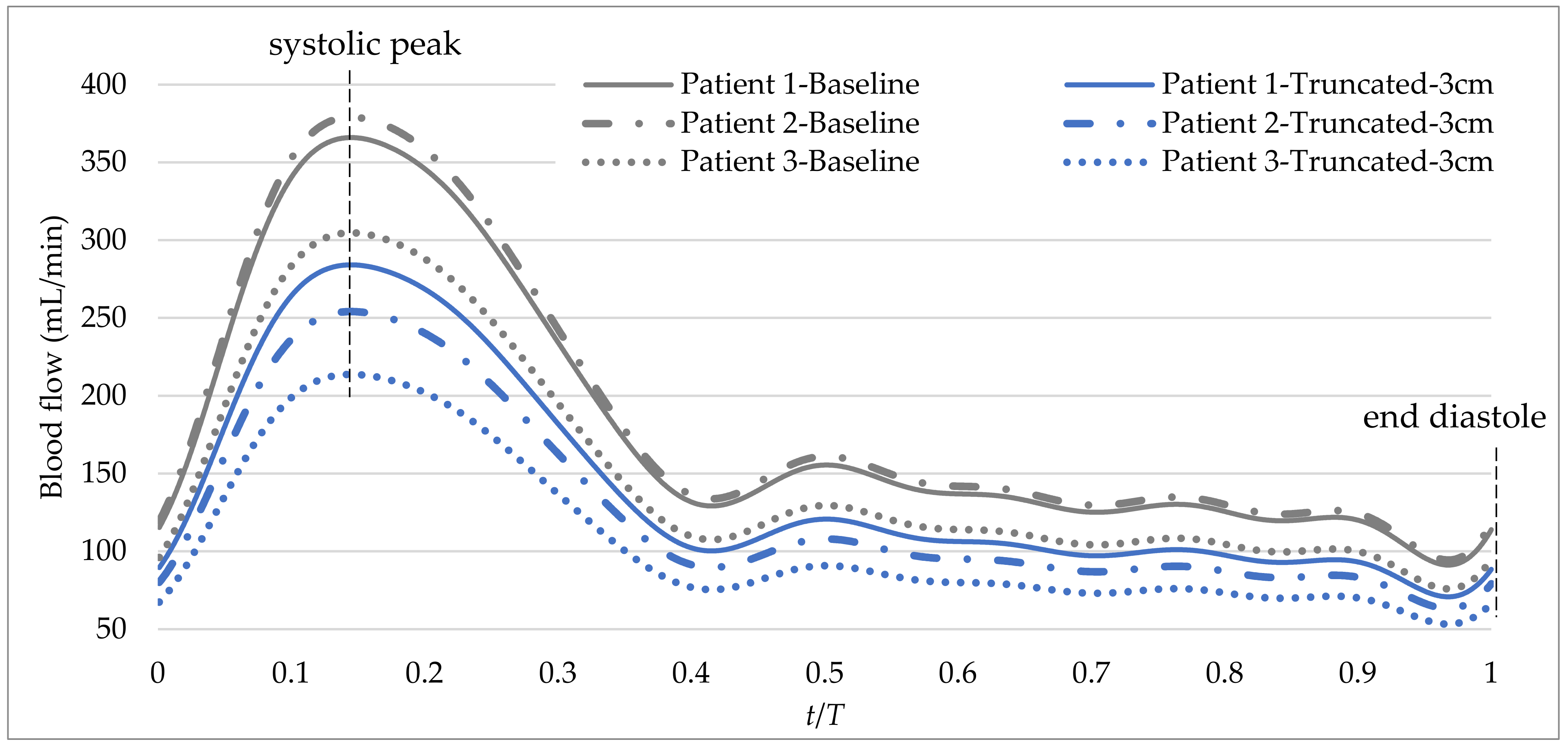
• Cycle-to-cycle computational time: to quantitatively assess the cost (in time) of each of the cycles.
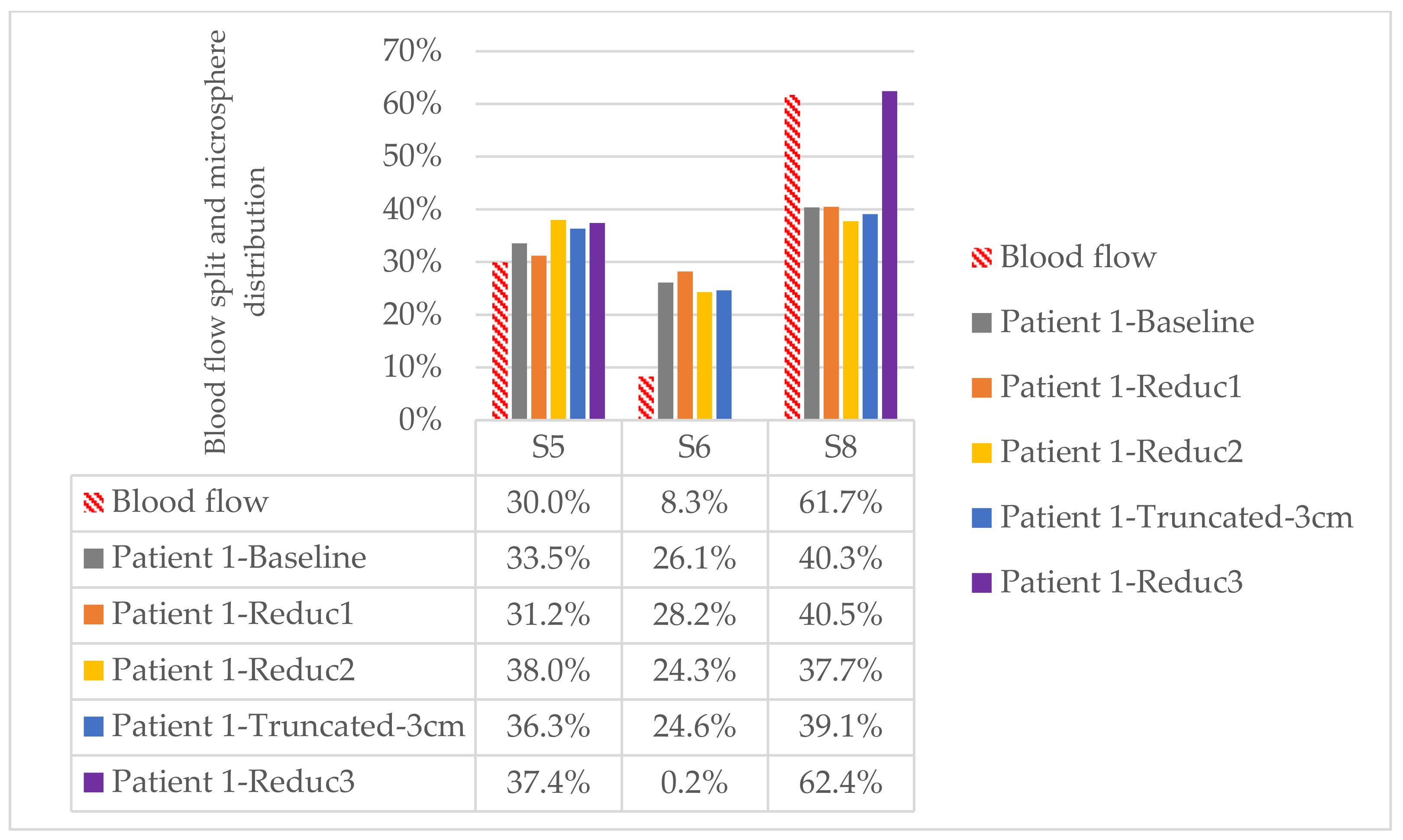
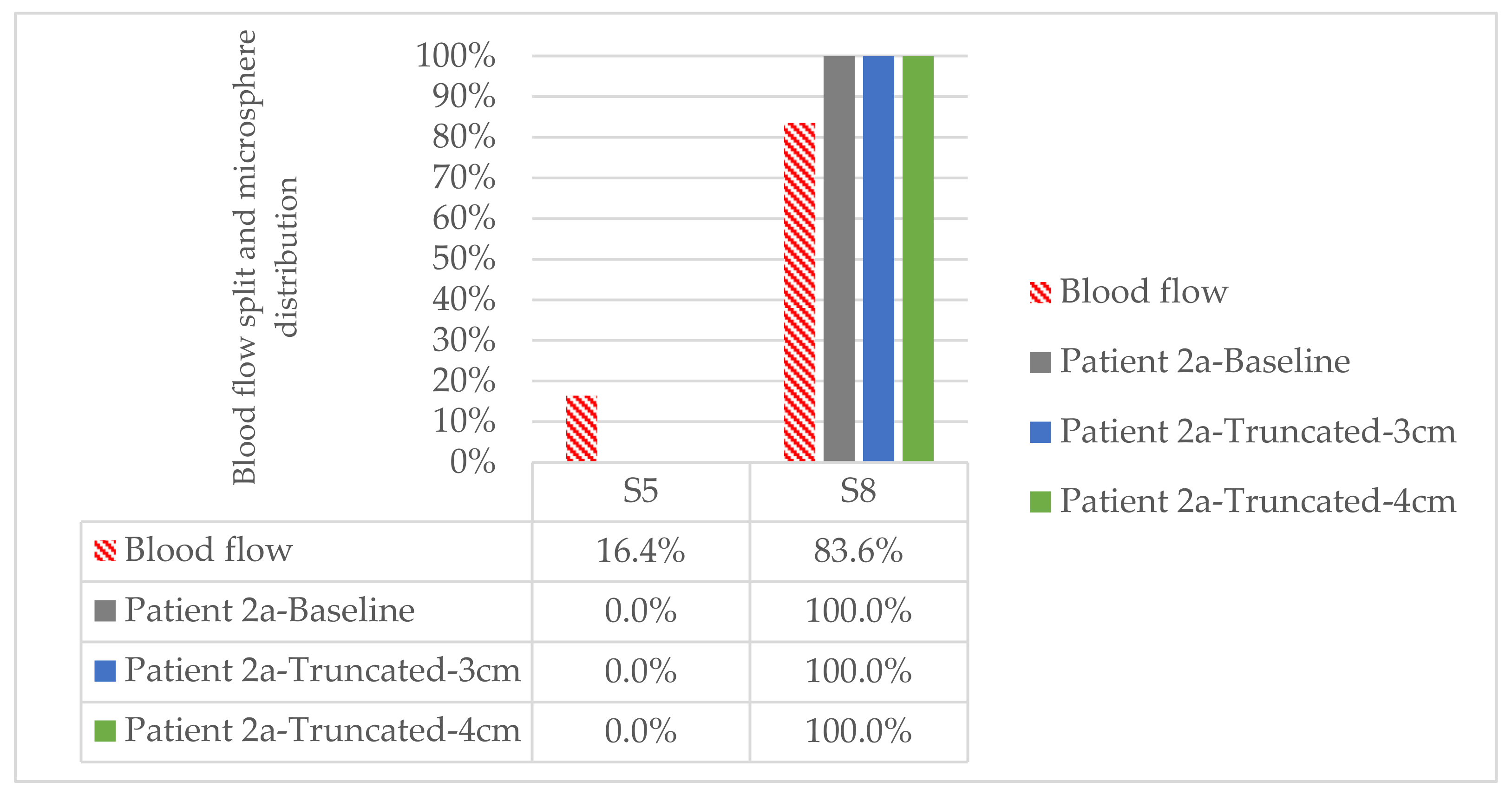
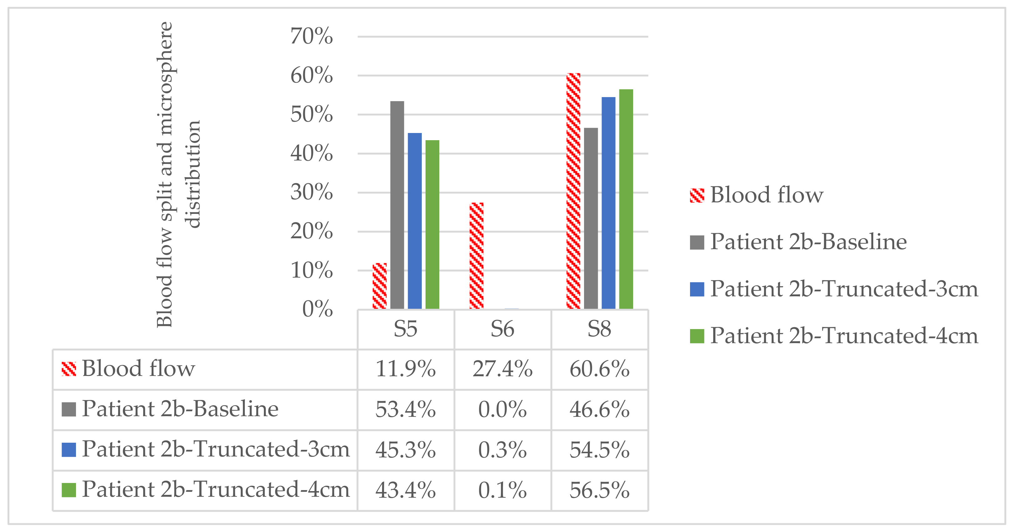
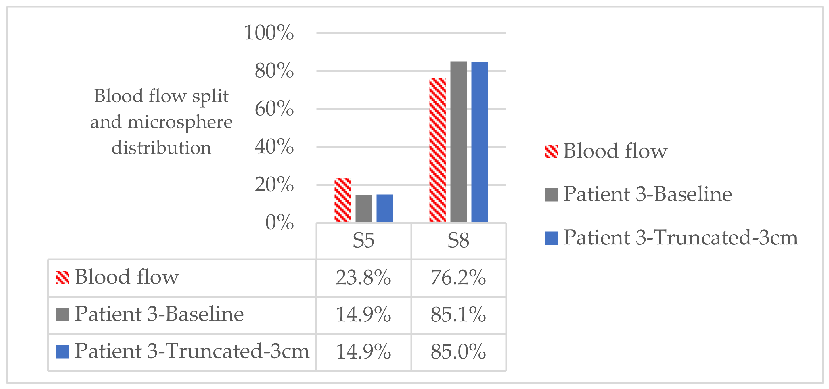
• Segment-to-segment microsphere distribution: to qualitatively assess the segment-to-segment microsphere distribution at the end of the treatment. This is calculated from the cumulative number of microspheres exiting through each outlet. The final outlet-to-outlet microsphere distribution is translated into the segment-to-segment microsphere distribution, which is the important parameters due to its clinical implication.
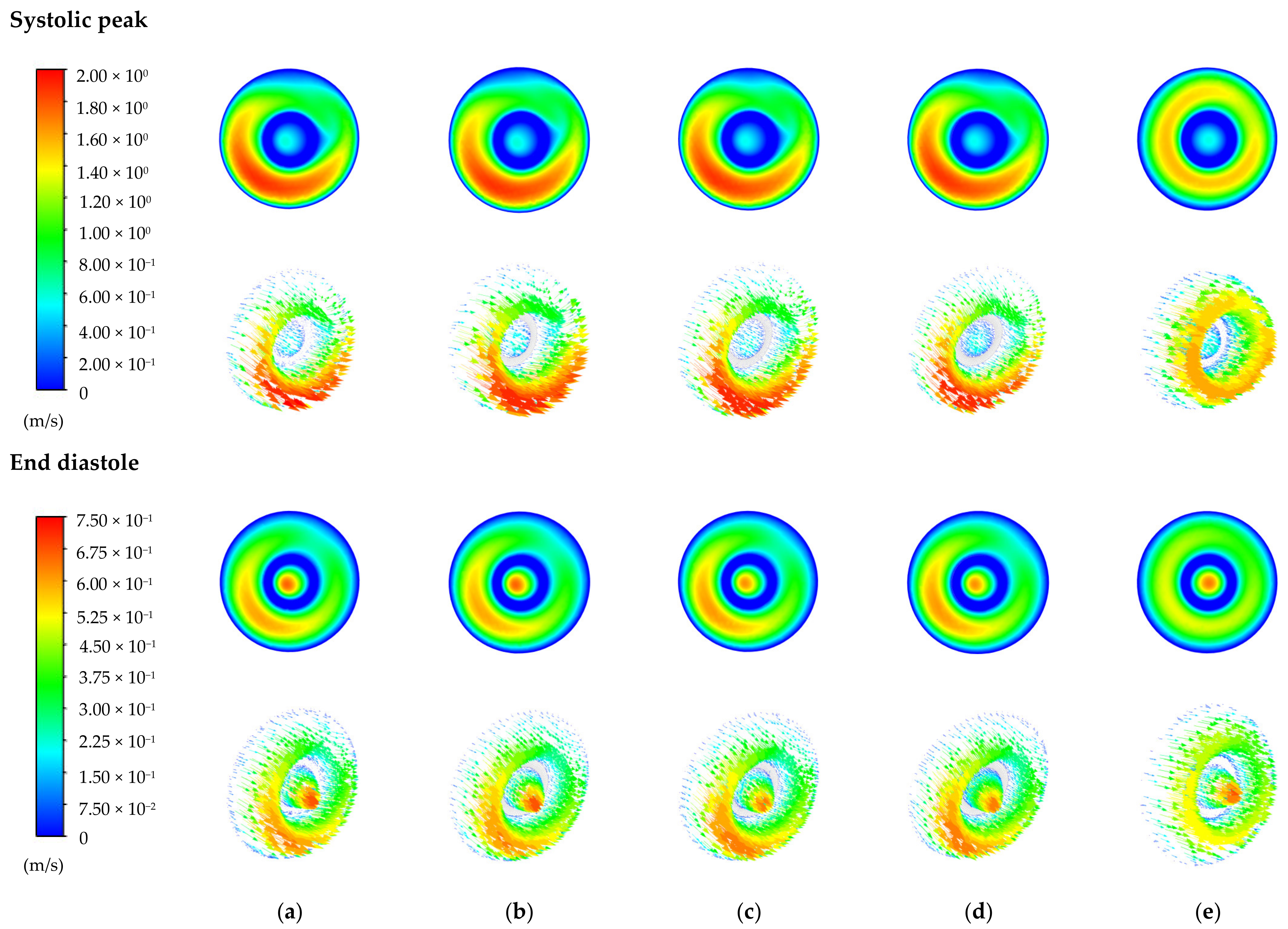
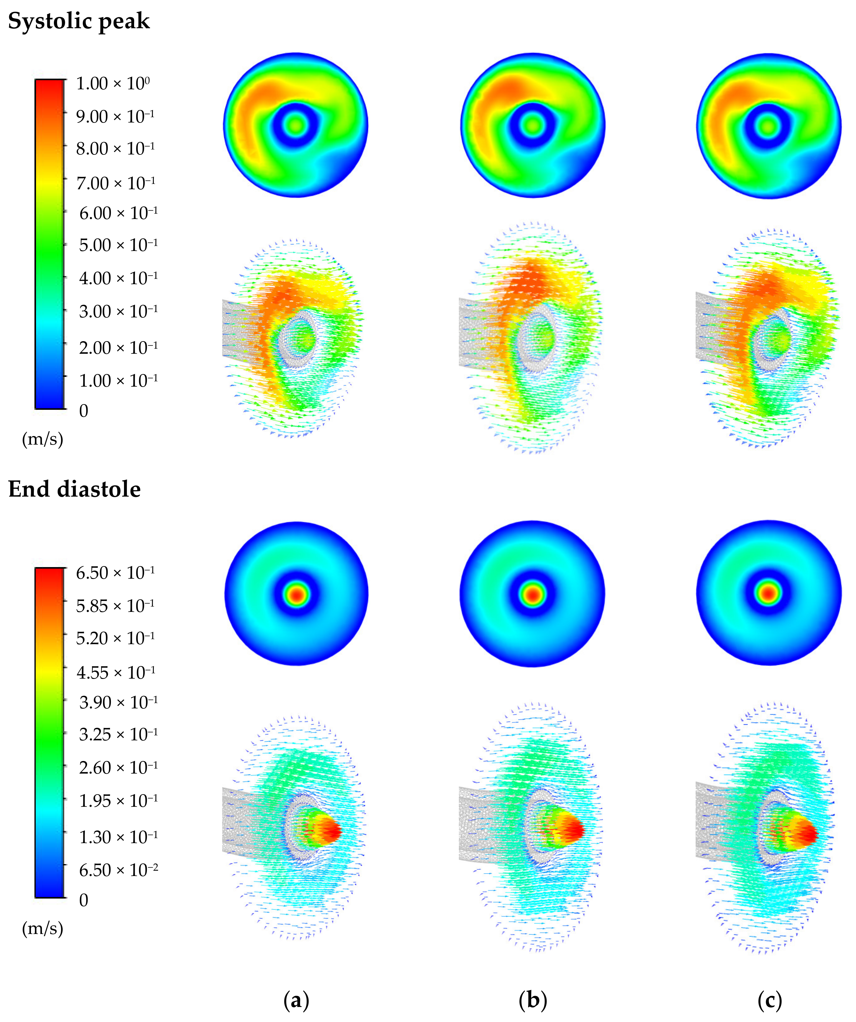
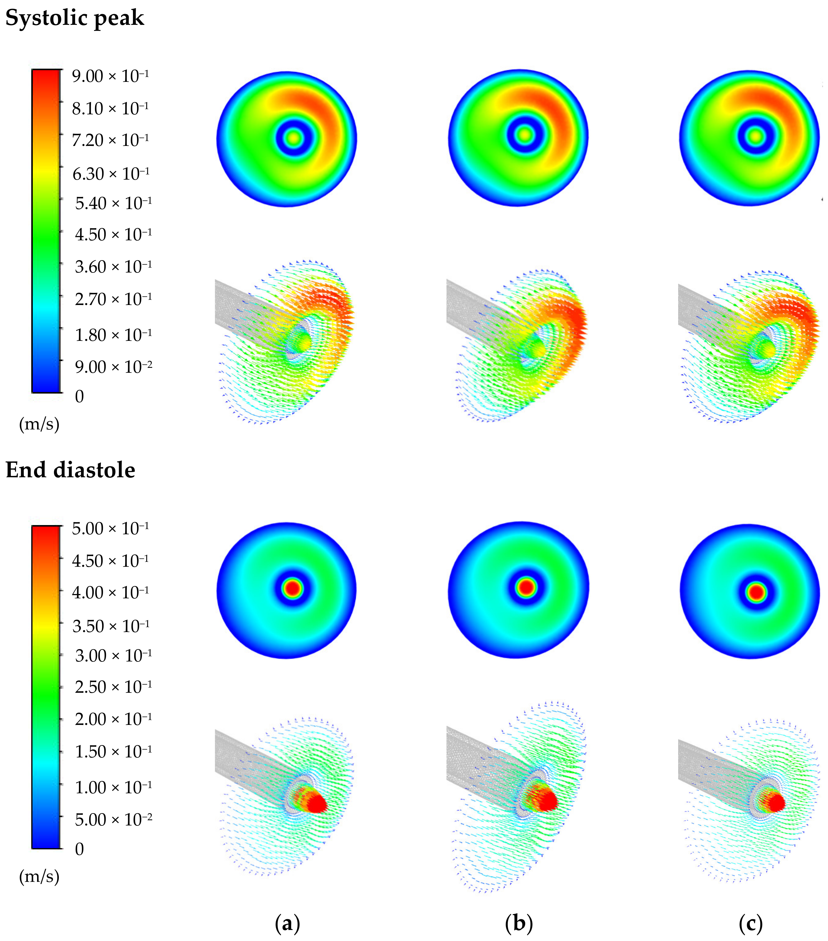
• Velocity magnitude contours and velocity vectors at the systolic peak and end diastole (see Figure 3) at the cross-section of the microcatheter tip: to qualitatively analyze important changes in the blood-flow pattern near the microcatheter tip. The important postprocessing is the segment-to-segment microsphere distribution for its clinical implications, but blood-flow patterns should be similar between the baseline and truncated geometries so that the microsphere distribution is also similar.

3. Results

For each patient, blood flow velocity magnitude contours and vectors at the cross-sectional plane of the microcatheter tip of baseline and truncated geometries are presented, together with segment-to-segment prescribed blood flow split and calculated microsphere distributions. These results are in Figure 4 and Figure 5 for Patient 1, Figure 6 and Figure 7 for Patient 2a, Figure 8 and Figure 9 for Patient 2b, and Figure 10 and Figure 11 for Patient 3. Figure 5, Figure 7, Figure 9 and Figure 11 show the distribution of the microspheres that exit the computational domain toward the segments. These values are normalized with respect to the total number of microspheres that exit the computational domain. In order to be able to compare the blood flow split and the microsphere distribution, blood flow values have been normalized with the blood flow through the artery branch where the microcatheter tip is located. It is important to note that microsphere and blood flow distributions are given in percentage values. When reporting differences between these magnitudes at a given segment, the absolute difference is reported, with units being percent points (%). The computational cost is also studied, focusing on the number of cardiac cycles required for microspheres to exit the computational domain and on the time reduction due to geometry simplification.

3.1. Patient 1

Figure 4 shows minor differences in velocity magnitude contours and velocity vectors between Patient 1-Baseline and almost all simplified cases except for Patient 1-Reduc3. Regarding this last case, Patient 1-Reduc3, blood flow patterns near the microsphere injection location have changed considerably because of an excessive geometry reduction. This change in blood flow pattern translates into differences in microsphere distributions. In fact, differences of 3.9%, 25.9%, and 33.9% are observed in S5, S6, and S8, respectively, between Patient 1-Baseline and Patient 1-Reduc3 (see Figure 5). With the defined criterion where a threshold of 10 percent points is taken as the maximum difference we can accept at a segment, then the simplification done for Patient 1-Reduc3 is unacceptable.

However, if we compare Patient 1-Baseline and Patient 1-Truncated-3cm, where no considerable differences are seen in velocity contours and vectors (see Figure 4), the differences in microsphere distributions are 2.8% in S5, 1.5% in S6, and 1.2% in S8 (see Figure 5). The maximum difference in percent points is below 3%, so this case is regarded as a case with a valid geometry truncation. As explained before, the same simplification criteria used to create Patient 1-Truncated-3cm was used in Patients 2 and 3, to analyze the usefulness of the criteria.

3.2. Patient 2

Additional geometries were generated for Patient 2a and 2b, after observing the differences in velocity contours and vectors in Patient 2a (see the high-velocity regions in the systolic peak contours in Figure 6a,b) and in microsphere distributions for Patient 2b (see Figure 9). For the additional truncated geometries, an extra centimeter was left in the geometries, resulting in a truncation of all the upstream branches farther than 4 cm from the microcatheter tip.

3.2.1. Patient 2a

Figure 6 shows differences between Patient 2a-Baseline and Patient 2a-Truncated-3cm velocity magnitude contours and vectors in the systolic peak (see the area of the high-velocity regions Figure 6a,b). This could potentially result in differences at the injection conditions and therefore in the microsphere distribution. As explained before, an extra case with an extra upstream centimeter was built to assess this difference. Indeed, Figure 6c shows that the results of Patient 2a-Truncated-4cm improve compared to Patient 2a-Truncated-3cm. Regarding the segment-to-segment microsphere distributions, all the cases show a S8-directed treatment (i.e., 100% microspheres targeting S8). Thus, even though some minor qualitative differences can be seen between Patient 2a-Baseline and Patient 2a-Truncated-3cm, the latter can be taken as valid because no differences in microsphere distribution are observed.

3.2.2. Patient 2b

Figure 8 shows that velocity magnitude contours and vectors are similar in all cases. However, the segment-to-segment microsphere distributions differ (see Figure 9). Segment to segment microsphere distribution differences between Patient 2b-Baseline and Patient 2b-Truncated-3cm are 8.1% in S5, of 0.3% in S6, and 7.9% in S8.

As explained before, an extra case was generated due to these differences. An extra centimeter was left upstream, giving as a result of the case Patient 2b-Truncated-4cm. The differences between Patient 2b-Baseline and Patient 2b-Truncated-4cm are 10% in S5, of 0.1% in S6, and 9.9% in S8. It is important to note that even though smaller truncation is applied in Patient 2b-Truncated-4cm, the differences with respect to the baseline case increased, compared to the differences between Patient 2b-Truncated-3cm and the baseline case. Thus, the case Patient 2b-Truncated-3cm has been considered a valid simplification.

3.3. Patient 3

Results show similar qualitative results of velocity contours and vectors between Patient 3-Baseline and Patient 3-Truncated-3cm (see Figure 9), and segment-to-segment microsphere distributions match—a difference of 0.1 percent points is seen in the microspheres targeting S8, see Figure 10.

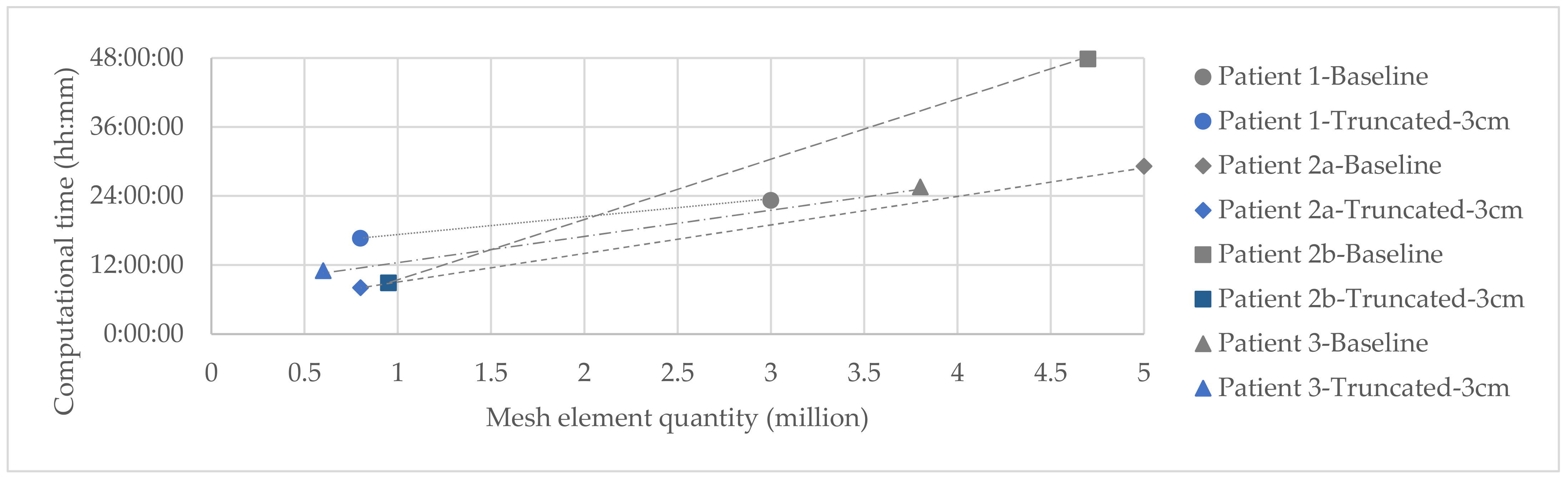
3.4. Computational Times

Reducing computational times by effectively reducing the hepatic artery geometry is the main goal of this study. In order to reduce the computational time, the size of the computational domain can be reduced. This reduction potentially allows for an additional reduction in simulation times because a smaller number of cardiac cycles are necessary to ensure that most of the injected microspheres exit the computational domain. Before carrying out the present study, a preliminary study was conducted to analyze the influence of the number of cardiac cycles simulated on the fraction of injected microspheres that exited the computational domain. The computational domains used in this preliminary study were not the same as the ones reported in the present study. Results can be regarded as representative because the baseline geometries are the same in the preliminary and actual studies and the reduced geometries are similar in the preliminary and actual studies. Figure 12 shows the fraction of microspheres that have exited the computational domain over time since the start of the injection—microspheres are injected between 0 s and 1 s, t = 1 s is the end of the first cycle (injection cycle) without microsphere injection t = 2 s is the end of the second cycle (extra cycle 1), etc.

Results show that in most cases a single extra cycle, i.e., extra cycle 1, is sufficient (t = 1–2 s) to achieve a steady number of the fraction of exited microspheres, but there are some baseline cases where a second extra cycle, i.e., extra cycle 2, is necessary (t = 2–3 s) (see Figure 12, Patient 2-Baseline and Patient 3-Baseline). The number of microspheres that exit the domain in extra cycles 3 and 4 (t = 3–5 s) are negligible. Accordingly, two extra cycles were considered in the simulations of the actual study. Hence, four cycles were necessary per simulation: an initial cardiac cycle for the blood flow convergence (t = −1 s to t = 0 s), another cycle to inject the microspheres (t = 0 s to t = 1 s), and two extra cycles (t = 1 s to t = 3 s).

For the simulations reported in the actual study, the computational time (i.e., cost) per cycle was analyzed and the cost of each cycle was assessed.

Table 5. Average relative computational time of each cardiac cycle of the simulation.

Cycle	Relative Computational Time
Cycle 1: Convergence	11.6%
Cycle 2: Injection	34.1%
Cycle 3: Extra cycle 1	28.0%
Cycle 4: Extra cycle 2	26.3%

collects the fraction of time needed for each cycle, averaged for the simulations presented in this article. Around 10% of the time is needed for the convergence cycle, a third of the time for the injection cycle, and half of the time for the extra cycles.

Finally, the relation between the number of mesh elements and the simulation duration was studied for the “Baseline” and “Truncated-3cm” geometries of the actual study, shown in Figure 13. The first observation is that simplifying the geometry results in a reduction in the computational time in all cases. This trend was expected due to the reduction in the number of mesh elements, but it can be quantified. The reduction in Patient 1 is from 23 h and 13 min to 16 h and 38 min (i.e., 28.4%); in Patient 2a, from 29 h and 11 min to 8 h and 03 min (i.e., 72.4%); in Patient 2b, from 47 h and 48 min to 8 h and 52 min (i.e., 81.5%); and in Patient 3, from 25 h and 35 min to 11 h and 00 min (i.e., 57%). Another observation is the fact that all the “Truncated-3cm” computational domains consist of a similar number of elements (near one million elements), even though the “Baseline” geometries differ in the number of elements. This comes as a result of applying the same geometry reduction strategy. It is also important to note that other factors that influence the simulation time include the quality of the elements of the mesh and the complexity of the studied blood flow.

4. Discussion

In this study, we analyzed the possibility of reducing the computational time of RE simulations by reducing the size of the geometry, without losing much accuracy in the segment-to-segment microsphere distribution prediction. For that purpose, three patient-specific hepatic artery trees were used. The geometry of the first patient was used as a case study to define a simplification strategy. This strategy consisted of removing from the computational domain branches that were upstream and downstream from the microcatheter tip. For upstream branches, all the branches that were farther than 3 cm were removed; for downstream branches, branches were removed at bifurcations where both daughter vessels fed the same liver segment.

The first observation is that the imposed blood flow split differs from the predicted or calculated microsphere distribution (see Figure 5, Figure 7, Figure 9 and Figure 11). This finding is not novel, it is indeed observed in previous studies that used a microcatheter to inject the microspheres [8] or the studies that used the particle release maps [7,9,26] as a research tool—particle release maps correlate each point in the injection cross-sectional plane with the computational domain outlet from which microspheres would exit. Even if a blood flow split-matching microsphere distribution can be achieved [5], this cannot be assumed as a general rule. Therefore, unless a blood flow split-matching microsphere distribution is promoted, CFD simulations are necessary to account for the influence of the local hemodynamic phenomena taking place during RE [3].

With regard to the geometry truncations, the four cases (Patient 1, Patient 2a, Patient 2b, and Patient 3) meet the criterion we established. It can be seen that the more tortuous and more intricate the geometry, the easier it is to obtain a good match between baseline and truncated simulations’ results. For Patient 1 and Patient 3, the biggest differences in microsphere distributions at a given segment are 2.8 and 0.1 percent points, respectively. These geometries are very tortuous, having bends close to 90° and bifurcations in the 3 cm of artery before the microcatheter tip. Regarding Patient 2a, the microsphere distribution in the truncated geometry is the same as the one obtained in the baseline geometry, even though minor differences in blood flow conditions near the injection location are qualitatively seen. Patient 2b gives the worst results when the microsphere distributions are compared in the baseline and truncated cases. However, the established criterion is still met. In these Patient 2 cases, the geometry has neither bifurcations nor large tortuosity in its initial part, supporting the hypothesis that the more the intricacies, the easier to replicate the baseline flow patterns in the simplified geometries. Therefore, it could be concluded that if the blood flow is intricate inside the 3 cm between the microcatheter tip and the upstream truncation, then the results of the truncated geometry will match better to the baseline geometry than if it is not.

Regarding the computational time analysis, it has been first concluded that two extra cycles are enough to ensure the fraction of exited microspheres reach a steady value over time (see Figure 12), and a four-cycle simulation is proposed: the first cycle for blood flow convergence, the second cycle for microsphere injection, and the third and fourth cycles for microspheres to exit the computational domain. Regarding the fraction of injected microspheres that do not exit the baseline computational domain, these values are 13.8%, 18.4%, 17.3%, and 9.7% for Patient 1, Patient 2a, Patient 2b, and Patient 3, respectively. These values are similar to those reported by Bomberna et al. [9]. In the truncated geometries, the fraction of non-exiting microspheres reduces to 13.8%, 0%, 6.2%, and 7.6% for Patient 1, Patient 2a, Patient 2b, and Patient 3, respectively. The simulation time of the baseline cases was 31 h 26 min on average, and that of the truncated cases 11 h 08 min on average (see Figure 13), meaning an average reduction of 64.6%. The comparison with other studies in the literature is tricky because the simulation time depends on the modeling approach and on the computer used to solve the model. Among the models used in the literature to study RE, the most similar one to the present model is that of Aramburu [27], with simulations taking 100 h approximately. Other similar models took 11–14 h [12] and around 38 h [7]. Other models have considered reduced order 1D and 0D models, resulting in simulations times of 1 h [28] and 5 s [29], respectively. However, these last models cannot capture local effects, which are essential in the microsphere distribution unless blood flow split-matching microsphere distribution is promoted. In the present case, the simulations have been carried out on a server with 80 cores and 125 GB of RAM. Although with this reduction it is possible to simulate the CFD model in half a day, it is still considered an excessive time for a feasible CFD-based computer platform. It is necessary to reduce more the computational time to offer to the treatment planning multidisciplinary team a versatile CFD-based computer platform to plan the intervention based on a patient-specific basis, being able to adjust the dosimetry with greater accuracy, potentially increasing the effectiveness of the intervention.

From the clinical point of view, we have posited a cancer scenario and we have placed the microcatheter at a reasonable location to target the tumor-bearing segment 8. Once we have performed the analysis with the aim of reducing the simulation time, we should analyze the results from the medical point of view. Results show that in the reduced geometries, the fraction of exiting microspheres targeting segment 8 are 39.1%, 100%, 54.5%, and 85%, for Patient 1, Patient 2a, Patient 2b, and Patient 3, respectively. When seeking to preserve as much healthy liver as possible, the aim is to advance the microcatheter as distally as possible. This allows to deliver high radiation doses via the microspheres released in the tumor-feeding arteries [2]. In this study, the site of injection of microspheres is optimal in Patient 2a, with 100% of microspheres reaching segment 8, and acceptable in the case of Patient 3 with 85% of microspheres reaching the tumoral segment (S8). This is not the case for the remaining cases. In Patient 1 and Patient 2b most of the radioactive load is directed to healthy tissue, with only 40% and 50% of the microspheres reaching segment 8, respectively. Patient 2 shows the importance of a correct microcatheter longitudinal location. In the case Patient 2a, 100% of the microspheres reach the tumor-bearing segment, whereas in the case of Patient 2b only 50% reach the target segment. However, the aim of the study was not to optimize the microcatheter location for an optimal microsphere delivery, but to assess the possibility of reducing the computational time by reducing the size of the simulated geometry. Moreover, results show that there is room for improvement and the microcatheter location could be modified in the simulations to improve the segment 8 targeting via simulation-based assessment. Again, the local effects would probably play an important role in the microsphere distribution and it would be very difficult to mimic the exact microcatheter location during the actual treatment.

Study Limitations

There are some limitations to this study. Regarding the modeling approach, patient-specific hepatic arteries have been used, but the hepatic and cancer states have been posited, with tumors localized in segment 8. Moreover, the first seconds have been taken as representative of the treatment that usually lasts half an hour—computationally unaffordable—without considering the microembolic effect of microspheres.

Regarding the methodology, only three patients—which can be seen as four cases—have been tested. Further research is needed to make sure that the rule works in most cases. Moreover, how to further reduce the computational time should be explored in future studies.

5. Conclusions

In the numerical simulation of RE, a patient-specific CFD analysis is necessary to capture in detail the influence of local effects near the injection location in order to predict the segment-to-segment microsphere distribution. Besides, the rule created to shorten the geometry of the hepatic artery for simulating the microsphere–hemodynamics during RE has resulted in simulations with differences smaller than 10 percent points in a given segment between segment-to-segment microsphere distribution results of the baseline and truncated geometries, as a result of minor changes in blood flow patterns, allowing for an important reduction in simulation time—in this study, an average time reduction of 62%. This simulation time reduction could be a step forward in the development of a simulation-based tool to be used in the clinical setting for personalized RE therapy planning to optimize the treatment.

References

1. Bray, F.; Ferlay, J.; Soerjomataram, I.; Siegel, R.L.; Torre, L.A.; Jemal, A. Global cancer statistics 2018: GLOBOCAN estimates of incidence and mortality worldwide for 36 cancers in 185 countries. CA Cancer J. Clin. 2018, 68, 394–424. [Google Scholar] [CrossRef] [Green Version]
2. Bajwa, R.; Madoff, D.C.; Kishore, S.A. Embolotherapy for Hepatic Oncology: Current Perspectives and Future Directions. Dig. Dis. Interv. 2020, 4, 134–147. [Google Scholar] [CrossRef]
3. Aramburo, J.; Antón, R.; Rivas, A.; Ramos, J.C.; Sangro, B.; Bilbao, J.I. Liver Radioembolization: An Analysis of Parameters that Influence the Catheter-Based Particle-Delivery via CFD. Curr. Med. Chem. 2020, 27, 1600–1615. [Google Scholar] [CrossRef]
4. Xu, Z.; Jernigan, S.; Kleinstreuer, C.; Buckner, G.D. Solid Tumor Embolotherapy in Hepatic Arteries with an Anti-reflux Catheter System. Ann. Biomed. Eng. 2015, 44, 1036–1046. [Google Scholar] [CrossRef] [PubMed]
5. Aramburu, J.; Antón, R.; Rivas, A.; Ramos, J.C.; Sangro, B.; Bilbao, J.I. Computational assessment of the effects of the catheter type on particle–hemodynamics during liver radioembolization. J. Biomech. 2016, 49, 3705–3713. [Google Scholar] [CrossRef]
6. Aramburu, J.; Antón, R.; Rivas, A.; Ramos, J.C.; Sangro, B.; Bilbao, J.I. The role of angled-tip microcatheter and microsphere injection velocity in liver radioembolization: A computational particle–hemodynamics study. Int. J. Numer. Methods Biomed. Eng. 2017, 33. [Google Scholar] [CrossRef] [PubMed]
7. Basciano, C.A.; Kleinstreuer, C.; Kennedy, A.S.; Dezarn, W.A.; Childress, E. Computer Modeling of Controlled Microsphere Release and Targeting in a Representative Hepatic Artery System. Ann. Biomed. Eng. 2010, 38, 1862–1879. [Google Scholar] [CrossRef]
8. Aramburu, J.; Antón, R.; Rivas, A.; Ramos, J.C.; Sangro, B.; Bilbao, J.I. Computational particle-haemodynamics analysis of liver radioembolization pretreatment as an actual treatment surrogate. Int. J. Numer. Methods Biomed. Eng. 2016, 33, e02791. [Google Scholar] [CrossRef] [PubMed]
9. Bomberna, T.; Koudehi, G.A.; Claerebout, C.; Verslype, C.; Maleux, G.; Debbaut, C. Transarterial drug delivery for liver cancer: Numerical simulations and experimental validation of particle distribution in patient-specific livers. Expert Opin. Drug Deliv. 2020, 1–14. [Google Scholar] [CrossRef] [PubMed]
10. Kleinstreuer, C. Drug-targeting methodologies with applications: A review. World J. Clin. Cases 2014, 2, 742–756. [Google Scholar] [CrossRef]
11. Roncali, E.; Taebi, A.; Foster, C.; Vu, C.T. Personalized Dosimetry for Liver Cancer Y-90 Radioembolization Using Computational Fluid Dynamics and Monte Carlo Simulation. Ann. Biomed. Eng. 2020, 48, 1499–1510. [Google Scholar] [CrossRef] [PubMed]
12. Childress, E.M.; Kleinstreuer, C. Impact of Fluid–Structure Interaction on Direct Tumor-Targeting in a Representative Hepatic Artery System. Ann. Biomed. Eng. 2013, 42, 461–474. [Google Scholar] [CrossRef] [PubMed]
13. Couinaud, C. The anatomy of the liver. Ann. Ital. Chir. 1992, 63, 693–697. [Google Scholar] [PubMed]
14. Oktar, S.O.; Yücel, C.; Demirogullari, T.; Uner, A.; Benekli, M.; Erbas, G.; Ozdemir, H. Doppler Sonographic Evaluation of Hemodynamic Changes in Colorectal Liver Metastases Relative to Liver Size. J. Ultrasound Med. 2006, 25, 575–582. [Google Scholar] [CrossRef] [PubMed]
15. Mise, Y.; Satou, S.; Shindoh, J.; Conrad, C.; Aoki, T.; Hasegawa, K.; Sugawara, Y.; Kokudo, N. Three-dimensional volumetry in 107 normal livers reveals clinically relevant inter-segment variation in size. HPB 2014, 16, 439–447. [Google Scholar] [CrossRef] [Green Version]
16. Aramburu, J.; Antón, R.; Rivas, A.; Ramos, J.C.; Sangro, B.; Bilbao, J.I. Liver cancer arterial perfusion modelling and CFD boundary conditions methodology: A case study of the haemodynamics of a patient-specific hepatic artery in literature-based healthy and tumour-bearing liver scenarios. Int. J. Numer. Methods Biomed. Eng. 2016, 32, e02764. [Google Scholar] [CrossRef]
17. Yang, H.F.; Du, Y.; Ni, J.X.; Zhou, X.P.; Li, J.D.; Zhang, Q.; Xu, X.X.; Li, Y. Perfusion computed tomography evaluation of angiogenesis in liver cancer. Eur. Radiol. 2010, 20, 1424–1430. [Google Scholar] [CrossRef]
18. Tsushima, Y.; Funabasama, S.; Aoki, J.; Sanada, S.; Endo, K. Quantitative perfusion map of malignant liver tumors, created from dynamic computed tomography data. Acad. Radiol. 2004, 11, 215–223. [Google Scholar] [CrossRef]
19. Sirtex Medical Limited. SIR-Spheres ® Y-90 Resin Microspheres (Yttrium-90 Microspheres). Available online: https://www.google.com/url?sa=t&rct=j&q=&esrc=s&source=web&cd=&ved=2ahUKEwjVj_uy4dzuAhVxRhUIHe0VCrUQFjAAegQI-Ax-AC&url=https%3A%2F%2Fwww.sirtex.com%2Fmedia%2F169247%2Fssl-us-14-sir-spheres-microspheres-ifu-us.pdf&usg=AOvVaw1W0waSBfewI6noitPu_xzW (accessed on 9 February 2021).
20. Kenner, T. The measurement of blood density and its meaning. Basic Res. Cardiol. 1989, 84, 111–124. [Google Scholar] [CrossRef]
21. Basciano, C.A. Computational Particle-Hemodynamics Analysis Applied to an Abdominal Aortic Aneurysm with Thrombus and Microsphere-Targeting of Liver Tumors. Ph.D. Thesis, North Carolina State University, Raleigh, NC, USA, 2010. [Google Scholar]
22. Basciano, C.A.; Kleinstreuer, C.; Kennedy, A.S. Computational Fluid Dynamics Modeling of 90Y Microspheres in Human Hepatic Tumors. J. Nucl. Med. Radiat. Ther. 2011, 1. [Google Scholar] [CrossRef]
23. Kleinstreuer, C.; Basciano, C.A.; Childress, E.M.; Kennedy, A.S. A New Catheter for Tumor Targeting With Radioactive Microspheres in Representative Hepatic Artery Systems. Part I: Impact of Catheter Presence on Local Blood Flow and Microsphere Delivery. J. Biomech. Eng. 2012, 134. [Google Scholar] [CrossRef] [PubMed]
24. Childress, E.M.; Kleinstreuer, C.; Kennedy, A.S. A New Catheter for Tumor-Targeting with Radioactive Microspheres in Representative Hepatic Artery Systems—Part II: Solid Tumor-Targeting in a Patient-Inspired Hepatic Artery System. J. Biomech. Eng. 2012, 134. [Google Scholar] [CrossRef]
25. Childress, E.M.; Kleinstreuer, C. Computationally Efficient Particle Release Map Determination for Direct Tumor-Targeting in a Representative Hepatic Artery System. J. Biomech. Eng. 2013, 136. [Google Scholar] [CrossRef]
26. Antón, R.; Antoñana, J.; Aramburu, J.; Ezponda, A.; Prieto, E.; Andonegui, A.; Ortega, J.; Vivas, I.; Sancho, L.; Sangro, B.; et al. A proof-of-concept study of the in-vivo validation of a computational fluid dynamics model of personalized radioembolization. Sci. Rep. 2021, 11, 1–12. [Google Scholar] [CrossRef] [PubMed]
27. Aramburu, J. Liver Radioembolization: Computational Particle-Hemodynamics Studies in a Patient-Specific Hepatic Artery under Literature-Based Cancer Scenarios. Ph.D. Thesis, Universidad de Navarra, Pamplona, Spain, 2016. [Google Scholar]
28. Umbarkar, T.S.; Kleinstreuer, C. Computationally Efficient Fluid-Particle Dynamics Simulations of Arterial Systems. Commun. Comput. Phys. 2015, 17, 401–423. [Google Scholar] [CrossRef]
29. Aramburu, J.; Antón, R.; Rivas, A.; Ramos, J.C.; Larraona, G.S.; Sangro, B.; Bilbao, J.I. Numerical zero-dimensional hepatic artery hemodynamics model for balloon-occluded transarterial chemoembolization. Int. J. Numer. Methods Biomed. Eng. 2018, 34, e2983. [Google Scholar] [CrossRef]
Figure 1. Patient 1 hepatic artery tree simplifications: (a) Baseline geometry (i.e., Patient 1-Baseline); (b) Upstream branches truncation (i.e., Patient 1-Reduc1); (c) Upstream truncation, 3 cm from the microcatheter position (i.e., Patient 1-Reduc2); (d) Intra-segmental branches truncation (i.e., Patient 1-Truncated-3cm); (e) Truncation before the first upstream branch (i.e., Patient 1-Reduc3). PHA: proper hepatic artery; LHA: left hepatic artery; RHA: right hepatic artery. Arrowheads indicate microcatheter-tip location. Arrows indicate branches feeding the tumor-bearing segment. S1–S8 in each outlet indicates that all the downstream branches arising from that outlet feed that segment.
Mathematics 09 00839 g001
Figure 2. Patient 2 and Patient 3 hepatic artery trees: (a) Baseline geometries (i.e., Patient 2a-Baseline, Patient 2b-Baseline, and Patient 3-Baseline); (b) Truncated geometries (i.e., Patient 2a-Truncated-3cm, Patient 2b-Truncated-3cm, and Patient 3-Truncated-3cm). PHA: proper hepatic artery; LHA: left hepatic artery; RHA: right hepatic artery. Arrowheads indicate microcatheter-tip location. Arrows indicate branches feeding the tumor-bearing segment. S1–S8 in each outlet indicates that all the downstream branches arising from that outlet feed that segment.
Mathematics 09 00839 g002
Figure 3. Inlet volumetric blood flows. Systolic peak (t/T = 0.15, with T = 1 s) and end diastole (t/T = 1, with T = 1 s) are the points where the postprocessing is done.
Mathematics 09 00839 g003
Figure 4. Patient 1 velocity magnitude contours and vectors: (a) Baseline geometry (i.e., Patient 1-Baseline); (b) Upstream branches truncation (i.e., Patient 1-Reduc1); (c) Upstream truncation, 3 cm from the microcatheter position (i.e., Patient 1-Reduc2); (d) Intra-segmental branches truncation (i.e., Patient 1-Truncated-3cm); (e) Truncation before the first upstream branch (i.e., Patient 1-Reduc3).
Mathematics 09 00839 g004
Figure 5. Patient 1, segment-to-segment blood flow distribution (normalized with the blood flow through the artery branch where the microcatheter tip is located) and microsphere distributions in the segments downstream from the injection plane (percentage of microspheres that have reached each segment, normalized with the total number of microspheres that exited the computational domain).
Mathematics 09 00839 g005
Figure 6. Patient 2a velocity magnitude contours and vectors: (a) Baseline geometry (i.e., Patient 2a-Baseline); (b) Upstream truncation, 3 cm from the microcatheter-tip location, and downstream truncation, intra-segmental branches (i.e., Patient 2a-Truncated-3cm); (c) Upstream truncation, 4 cm from the microcatheter-tip location, and downstream truncation, intra-segmental branches (i.e., Patient 2a-Truncated-4cm).
Mathematics 09 00839 g006
Figure 7. Patient 2a, segment-to-segment blood flow distribution (normalized with the blood flow through the artery branch where the microcatheter tip is located) and microsphere distributions in the segments downstream from the injection plane (percentage of microspheres that have reached each segment, normalized with the total number of microspheres that exited the computational domain).
Mathematics 09 00839 g007
Figure 8. Patient 2b velocity magnitude contours and vectors: (a) Baseline geometry (i.e., Patient 2b-Baseline); (b) Upstream truncation, 3 cm from the microcatheter-tip location and downstream truncation, intrasegmental branches (i.e., Patient 2b-Truncated-3cm); (c) Upstream truncation, 4 cm from the microcatheter-tip location, and downstream truncation, intrasegmental branches (i.e., Patient 2b-Truncated-4cm).
Mathematics 09 00839 g008
Figure 9. Patient 2b, segment-to-segment blood flow distribution (normalized with the blood flow through the artery branch where the microcatheter tip is located) and microsphere distribution in the segments downstream from the injection plane (percentage of microspheres that have reached each segment, normalized with the total number of microspheres that exited the computational domain).
Mathematics 09 00839 g009
Figure 10. Patient 3 velocity magnitude contours and vectors: (a) Baseline geometry (i.e., Patient 3-Baseline); (b) Upstream truncation, 3 cm from the microcatheter-tip location, and downstream truncation, intra-segmental branches (i.e., Patient 3-Truncated-3cm).
Mathematics 09 00839 g010
Figure 11. Patient 3, segment-to-segment blood flow distribution (normalized with the blood flow through the artery branch where the microcatheter tip is located) and microsphere distributions in the segments downstream from the injection plane (percentage of microspheres that have reached each segment, normalized with the total number of microspheres that exited the computational domain).
Mathematics 09 00839 g011
Figure 12. Fraction of microspheres that exited the computational domain over time.
Mathematics 09 00839 g012
Figure 13. Computational time vs. mesh size.
Mathematics 09 00839 g013