1. Introduction
Landslide phenomena constitute an important natural hazard induced frequently by extreme rainfall and strong earthquakes. Landslides pose a major threat to the human life and natural environment, as well as to commercial and public infrastructure, having significant economic impact. According to recent research conducted in 27 European countries [
1], 1370 deaths and 784 injuries were recorded from 476 deadly landslide events during the 20 years period 1995–2014. In a continuously changing environment due to natural and anthropogenic factors (e.g., climate change, population growth, etc.), the landslide hazard determination is considered as decisively important.
On the one hand, there are techniques of landslide assessment that reduce time and cost consuming by applying simplified approaches, but they are based on low-resolution input data. On the other hand, the most robust models require landslide records that increase economic and time demands (e.g., in situ measurements, large volume of data, etc.). In the literature background, there are several methods for landslide susceptibility modeling, qualitative or quantitative, deterministic, or probabilistic approaches, empirical or heuristic. Landslide inventory is a basic input, which can be used for the landslide hazard model calibration and validation, enhancing the process consistency and efficiency.
SAR interferometry is a powerful tool for detection and monitoring of ground deformation phenomena [
2,
3,
4,
5,
6,
7] and can be proven as an efficient method to assist and update landslide inventory, especially in cases where such information is not available [
8,
9,
10,
11,
12,
13]. “In recent years, multiple remote sensing techniques, including synthetic aperture radar, optical and light detection and ranging measurements from space borne, airborne, and ground-based platforms, have been widely applied for the analysis of landslide processes” [
14]. Several studies evaluate landslide inventories based on remote sensing for landslide hazard or risk assessment [
15,
16,
17]. This study attempts to add further knowledge in this particular research field.
This paper presents a method that combines the deformation modeling through multi-temporal SAR technique with the landslide susceptibility modeling. At the first part of our analysis, a high temporal sampling rate of historical ERS-1/2 and ENVISAT SAR imagery is deployed by the multi-temporal interferometry (MTI) technique in order to update and enrich an existing well-established ground truth dataset with the diachronic MTI results. Additionally, it provides spatial and temporal information about landslide activity, detecting new or reactivated slope failures, mainly in remote mountainous areas.
In a probabilistic framework, the weights of evidence (WoE) method is selected for landslide susceptibility zones identification. It is widely used [
18,
19,
20,
21,
22,
23] due to its applicability and reliability combining different geospatial data and landslide inventory through a robust statistical approach. However, a variety of methods exist in the literature, such as bivariate and multivariate statistics approaches, e.g., frequency ratio [
24] and logistic regression [
25,
26], fuzzy approaches [
27], neural network model [
28,
29,
30], or integrated techniques [
31]. A significant advantage that WoE method provides is the estimation of the relative importance of landslide predisposing factors by statistical means.
In terms of landslide models, a question that arises∙ is about the capability to achieve the same or similar precision by using less data and more simplified methods. For this purpose, two different approaches are demonstrated and compared in order to detect any weaknesses but also their capabilities in landslide modeling. More specifically, the WoE method is compared to the Norwegian Geological Institute (NGI) method. The first one is applied at regional scale while the second one at global level.
This study’s outcome aims to present an integrated end-to-end approach providing a constantly updated landslide susceptibility map, useful for operational implications for mandated organizations. It must be pointed out that using sequential SAR image acquisitions, over the same area, is beneficial for the continuous update of the landslide inventory. This may prove to be a valuable operational tool for the authorities and protection agencies.
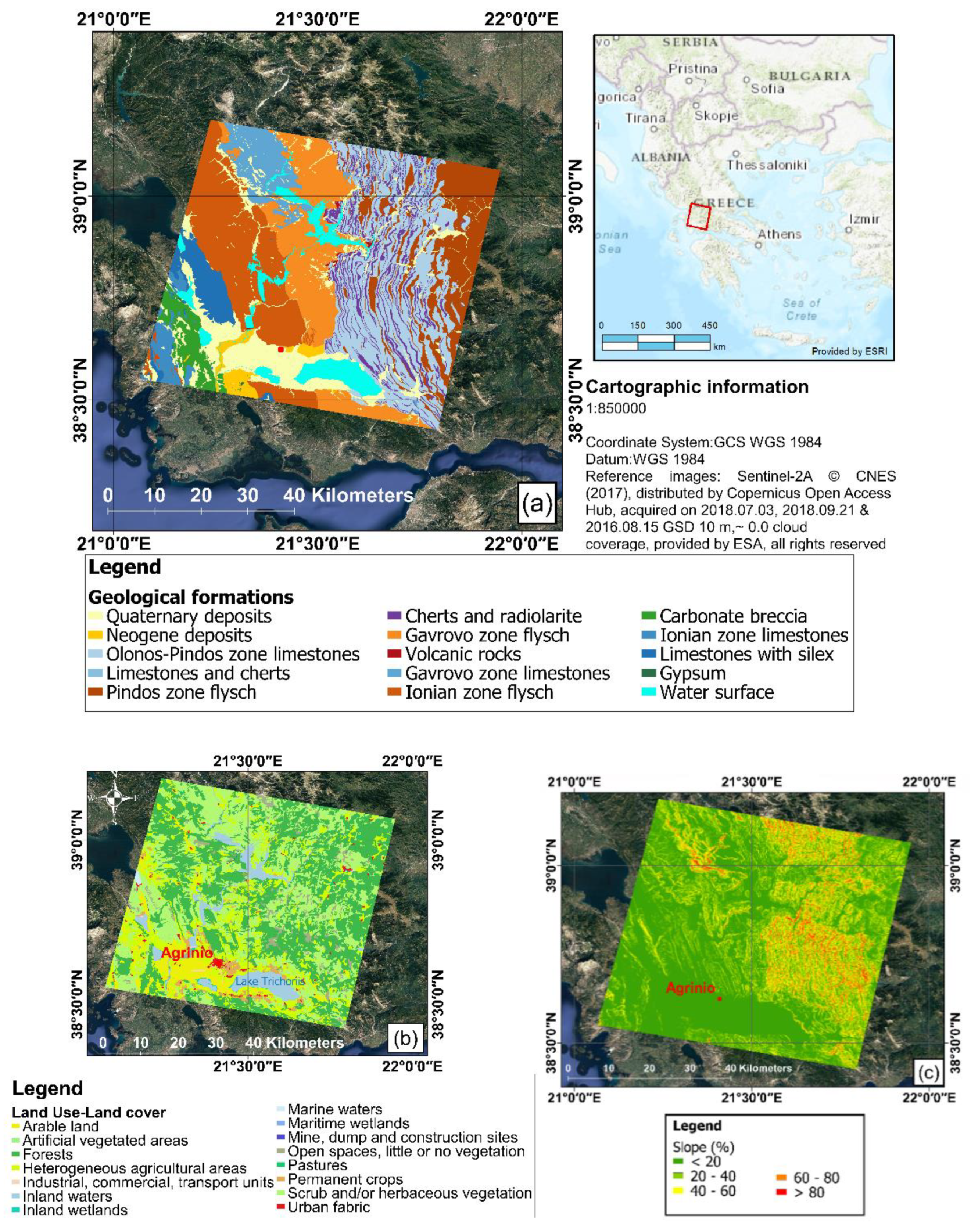
The study area selected for the application of the proposed methodology covers a big part of the Aetolia–Acarnania and Evritania prefectures, Central and Western Greece, aiming to include areas with both high and low landslide occurrence frequencies. In the following sections, a detailed description of the study area and the input data, the analysis of the applied methodologies referring to the interferometric based landslide inventorying and hazard modeling, and finally the returned results along with the presented conclusions, are presented.
2. Study Area
The study area is located in Central and Western Greece, a part of the Pindus mountain range. Extends over 4603 km
2 and covers mainly two prefectures, those of Aetolia–Acarnania and Evritania (
Figure 1) and three geotectonic zones, those of Pindos, Gavrovo, and Ionian [
32]. The area has been selected due to its wide variations in regards to the frequency of landslide occurrences, as Pindos geotectonic zone is characterized as the most landslide prone area of Greece while Gavrovo and Ionian present much lower landslide occurrence frequencies [
33,
34]. Specifically, Pindos geotectonic zone concentrates more than 40% of the total cases recorded in Greece, while Gavrovo and Ionian, 4% and 4.5%, respectively.
From a geotectonic point of view, Pindos, Gavrovo, and Ionian zones belong to the External Hellenides zones that occupy the central and the western part of Greece. The External Hellenides are occupied by formations younger than those of the Internal Hellenides, mainly Mesozoic sedimentary formations such as limestone and flysch [
32]. They are characterized by the presence of strong E–W tangential tectonic movements, resulting to a westward-directed ductile thrusting and intense folding and fracturing [
32,
35]. The faulting tectonism of the Alpine orogeny formed extensive trances that, during the Paleogene and the Neogene, were filed by Molasse and Marl formations, respectively [
32,
36,
37]. Furthermore, terrestrial, lacustrine, and river Quaternary deposits can be identified along the plain areas and coastal zone of the country. The tectonic disturbance of the geological formations of the External Hellenides zones constitutes an important landslide causal factor and the areas belonging to these zones exhibit high landslide susceptibility index [
33,
34].
The regional morphology is dominated by mountainous topography characterized by high elevation reaching 2290 m a.s.l. and dense hydrographic features. Additionally, at the Pindos geotectonic zone, the intensive tectonism due to the successive over-thrusts, the steep slopes, the highly landslide susceptible flysch formations (turbidity flow deposits of shales and sandstones) and the high precipitation levels enhance the occurrence of slope failures. On the contrary, the smooth mega-anticlines forming the mountains at the Gavrovo and Ionian geotectonic zones, the gentler tectonism, and the domination of limestone formations decrease substantially the landslide occurrence frequencies. Besides the geological complexity, the study area is characterized by a wide variety of land uses, such as forests, agricultural areas, shrubs, and herbaceous vegetation.
The climate at the highlands of the study area can be characterized as Alpine Mediterranean with harsh winters and cooler summers, with frequent thunderstorms. At the lowlands, western part of the study area, the climate is typical Mediterranean with wet winters and dry summers. At this point, it should be noted that the climate is wetter at the west side of the Pindus mountain range, while at the east is drier and windier in summer [
38]. Moreover, rainfall data of the last decade for Karpenisi, Agrinio, and Gavalou meteorological stations, obtained by the Institute for Environmental Research, National Observatory of Athens (IERSD/NOA) are provided in
Figure S1 (see Supplementary Material).
3. Input Data and Their Pre-Processing
3.1. Landslide Inventory
Landslide hazard assessment requires a complete landslide inventory. Landslide inventory is the most important input layer, as it gives an insight at the location of past landslide occurrences, as well as their failure mechanisms, causal factors, frequency of occurrence, volumes, and the damage that has been caused [
39]. The study area is affected by both slow-moving slides and creep movements as well as fast moving debris and earth flows (
Figure 2C), rock falls and toppling failures. The thick weathering mantle of the flysch formations is involved by deep-seated rotational slides (
Figure 2D) and extensive creep movements. Moreover, fast moving flows (
Figure 2A,B) occur during periods of prolong or intensive precipitation, due to the increase of the soil moisture and the proportional reduction of the shear strength of the flysch’s weathering mantle. Extensive planar failures along the bedding plains of the flysch formations also occur at the major anticline structures of the Ionian zone. On the other hand, the fractured rock formations (limestones, cherts, etc.) exhibit numerous debris flows (
Figure 2E,F), rock falls, and toppling failures mainly during periods with intensive weather events.
The current study intents to couple pre-existing landslide inventory based on field investigations with multi-temporal interferometry technique by exploiting ERS1/2 and ENVISAT historical time series datasets, in terms of displacements and average velocities measurements. The availability of pre-existing landslide inventory at the region of interest has been provided by the Hellenic Survey of Geology and Mineral Exploration (HSGME -former IGME-GR) covering the period from 1965 to 2010. The landslide historical records refer to cases where expert geologists have visited upon request for landslide in situ surveys mostly at residential areas or along transport or lifelines networks. Thus, the inventory consists mainly of events that have caused significant impact to infrastructure. The geological setting, as well as the geometry and the failure mechanisms, are available at the inventory for each failure.
Towards an updated landslide inventory, remote sensing plays a key role for landslide identification, monitoring, and mapping. Landslide boundaries confirmation and updating, new failures detection, and landslide activity evaluation are achieved due to the wide area coverage, of non-invasive and cost-effective remotely sensed data, [
40]. The valuable tool of multi-temporal interferometry technique has been implemented for the periods 1992–2000 and 2003–2010 using ERS1/2 and ENVISAT datasets, respectively, to detect extremely to slow moving landslides (according to velocity scale proposed by IGUS/WGL, 1995 [
41]). A serious limitation in the selection of the satellite tracks was data availability. For ENVISAT data, the ascending satellite pass could not provide the appropriate number of SAR images (a stack with >30 images), to ensure an accurate modeling of the interferometric signals. Therefore, we proceeded with the descending satellite pass for both ERS and ENVISAT data. Descending track 50 was selected for SAR processing. All available ERS1/2 and ENVISAT raw SAR images of descending tracks were analyzed to estimate mean line of sight displacements. Focusing of raw data, was performed with ROI_PAC software, with the use of orbital data from the Department of Earth Observation and space systems (DEOS) of the Delft University of Technology and the European Space Agency (ESA). We oversampled Single Look Complex (SLC) data by a factor of two in azimuth and range direction, to increase the number of coherent pixels. Finally, for the formation of differential interferograms DORIS software was used. The available inventory permits the spatial correlation of the MTI results with ground truth observations, leading to an updated inventory.
The correlation of the above-mentioned layers is also supported by conventional visual photo interpretation based on high-resolution imagery, covering all types of failures. The aim is to assess the geomorphological evidences and indicators (e.g., anomalies in vegetation coverage) introducing new landslide detections in locations with no previous evidence on landslide movements [
42]. Moreover, additional field visits were conducted for the validation of new landslide detections.
3.2. Static Geospatial Data
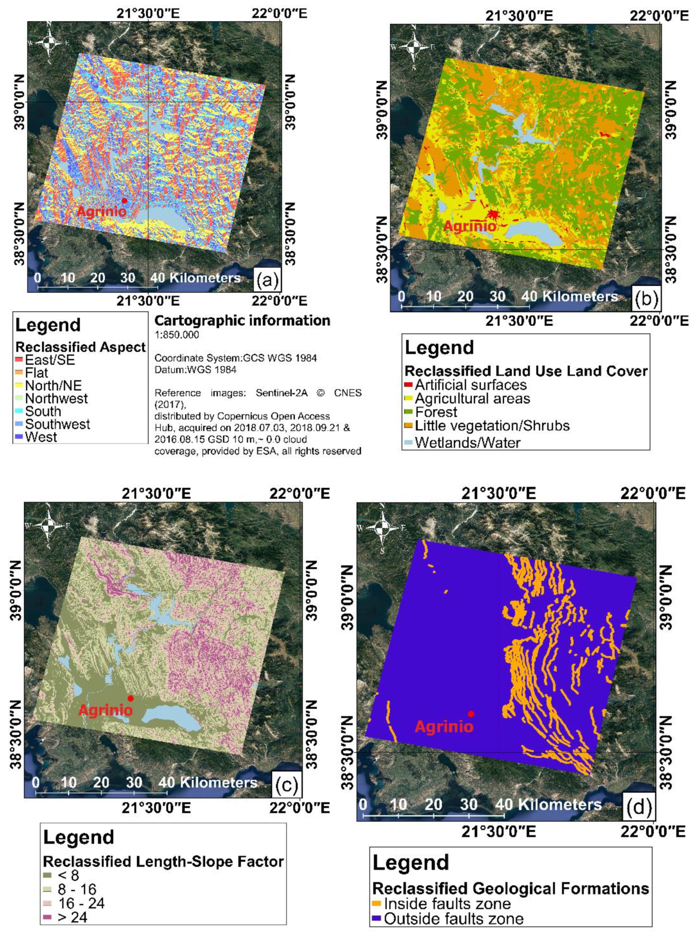
In addition to landslide inventory, predisposing factors poses as a crucial information layers to establish the link of the landslide spatial distribution with the topographic, geological, hydrological, and geomorphological settings of the area. Several thematic maps depicting geomorphological factors influenced by instabilities were generated for the statistical method of landslide susceptibility. Slope inclination, aspect, length–slope factor, and convexity maps are derived from DEM with resolution of 25 m × 25 m with vertical accuracy ±7 m RMSE (Root Mean Square Error), available from GMES RDA project (EU-DEM) [
43]. The accuracy of the Digital Elevation Model (DEM) has an impact on the generation of geomorphometric parameters. However, several studies [
44,
45,
46] conclude that high-resolution DEM does not always ensure higher slope and aspect accuracy. Land use land cover has proven to be an effective mitigation measure for rainfall-induced landslide, as it affects slope stabilization due to its mechanical and hydrological effects [
47]. The land use land cover layer used for the analysis is extracted by Corine Land Cover (CLC) 2012 version 18.5.1. In addition, digital geological features (e.g., geological formations, faults, etc.) were provided by HSGME) [
48]. The geological formations have been grouped according to their expected geo-mechanical behavior, and by considering the lithological characteristics and the tectonic strain and fragmentation of each geotectonic zone. Finally, a new layer has been created including the unified engineering geological formations [
49]. Moreover, buffer zones of 350 m have been created along shear zones as the geomechanical properties of rocks have been degraded along these zones. In
Figure 3, a list of thematic maps of the study area is presented.
3.3. Precipitation Data
Apart from the static geospatial data, the precipitation pattern of the study area is considered as a dynamic input for the landslide susceptibility estimation. In Greece, the topographic relief dominated by the Pindus mountain range, determines the rainfall amounts through the orographic effect the western side of mountains receives more rainfall than the eastern side.
Extreme rainfall is considered as a triggering factor for landslide events. The intensity–duration–frequency curves describe the mathematic relationship between maximum rainfall intensity, rainfall duration, and return period. Based on a probabilistic-statistic approach, they are derived from the frequency analysis of historical time series rainfall observations. They are widely used in hydrological and hydraulic design. The rainfall intensity–duration–frequency (IDF) curves incorporate the microclimate factors and vary from region to region.
In the current paper, the IDF relationships, provided by the Ministry of Environment and Energy in the framework of the flood risk assessment and management Directive 2007/60/EC [
50], are implemented on the rainfall stations of the area of interest. The study area spreads over three water districts, Epirus (GR05), Western Sterea Ellada (GR04), and Thessaly (GR08), including a total of 36 rainfall stations (
Figure 4). For a given storm duration of 24 h and return period of 50 years, rainfall intensity (mm/h) was calculated for each station included in
Figure 4, using the parameters (κ, λ, ξ, θ, ψ), of the most suitable distribution function for the highest rainfall intensity. Spatial interpolation of rainfall intensity data is conducted using Spline technique and the areal reduction factor are implemented in order to obtain the final rainfall pattern of the study area. In
Figure 4, we present the precipitation map derived from the observations of the in situ meteorological stations of 50 years return period for the study area, as a result of our analysis [
51,
52].
where
d is the duration of the rainfall, T is the return period, κ is the shape parameter, λ′ is the scale parameter, ψ′ is the position parameter of the distribution function, and θ, η are the parameters of the duration function.
4. Methodology and Data Analysis
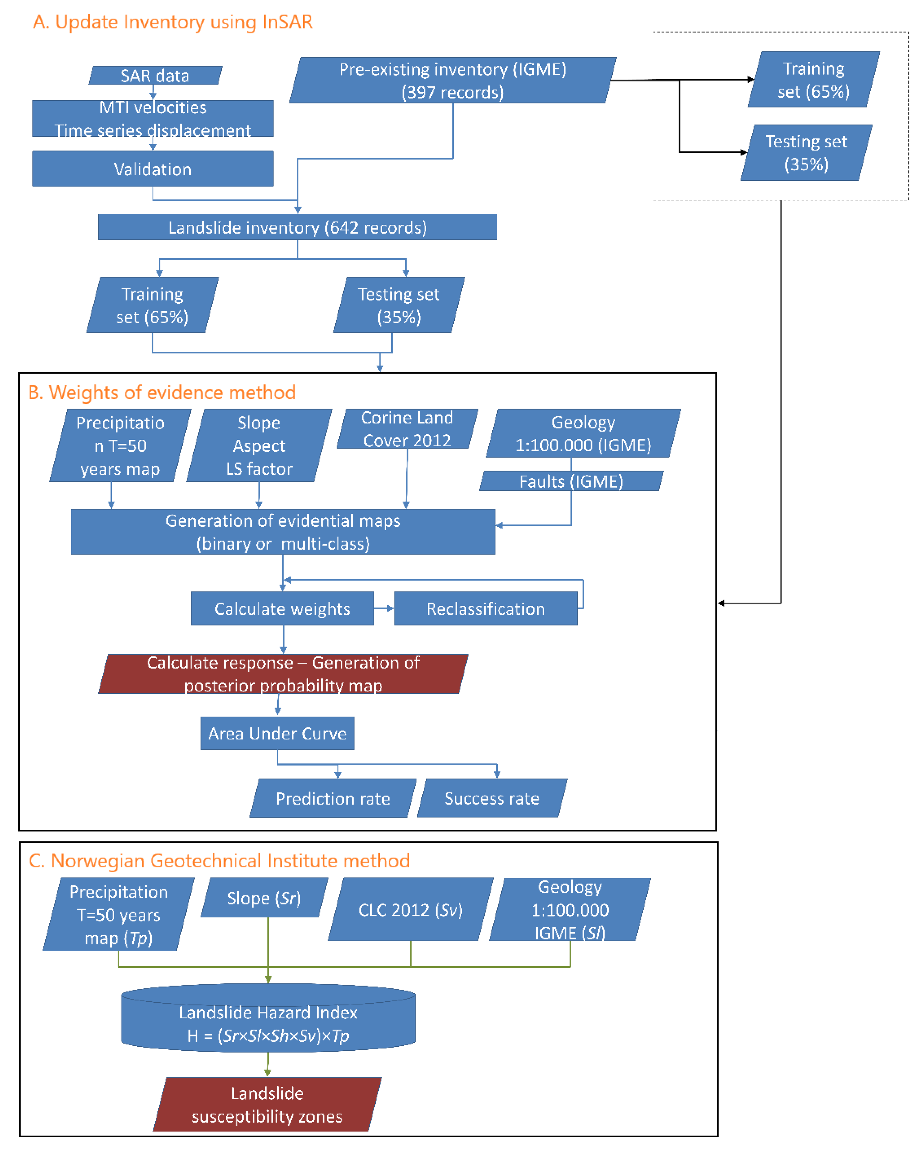
Following the updated landslide inventory, a statistical model versus a simplified model (
Figure 5) are implemented for landside susceptibility. In the probabilistic framework, a composite data-driven approach is applied in the regional-scale weights of evidence (WoE) method, in contrast to a simplified first-pass analysis–Norwegian Geotechnical Institute (NGI) method. Both methods are performed in a GIS environment. In particular, spatial data modeler (ArcSDM), an extension of ESRI’s ArcGIS software, is used for the statistical method implementation.
4.1. Landslide Inventory
4.1.1. Multi-Temporal Interferometry Technique
Pre-processing investigation showed that layover and shadowing image distortions were minimized for the descending satellite trajectory, and the track 50 was chosen as the most suitable for the analysis, to capture as many slopes as possible. Time series analysis was conducted by processing 53 SAR images of ERS1/2 sensors and 23 images of ENVISAT sensor, monitoring extremely to very slow-moving landslides. The open source software package StaMPS [
53] was used for the SAR images processing, by incorporating Persistent Scatterers [
54] and Small Baselines [
55], plus the option to combine both techniques [
56]. The persistent scatterer (PS) approach identified bare soil outcrops, semi-urban areas and infrastructures, whereas the small baseline subset (SBAS) approach provided additional coherent pixels in semi-vegetated and agricultural lands.
Table 1 presents explicitly the dataset used and the post-processing information.
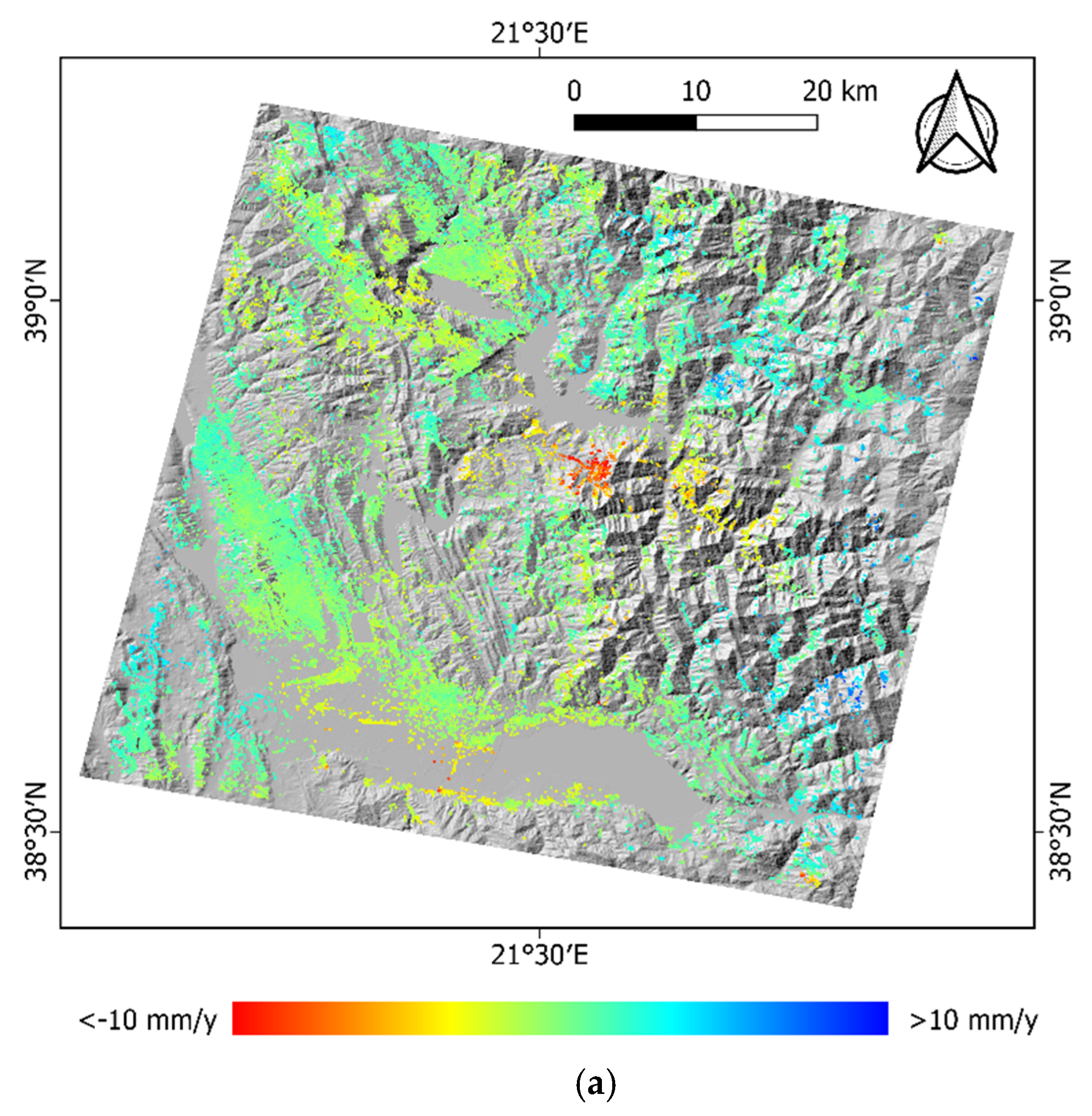
Figure 6 demonstrates the mean velocity values along the line of sight (LOS) for the periods 1992–2000 and 2003–2010 for ERS1/2 and ENVISAT sensors. The city of Agrinio was set as reference area, located to the West of Trichonis Lake. At higher altitudes, the MTI technique identifies slow sliding movements along slopes with steep gradients at bare rock outcrops, or soil scarps where vegetation interruption allows scatterers detection. It is important to point out that slope values greater than 20° were used as a threshold for the detection of deformation processes related to landslide phenomena. This threshold was applied aiming to exclude deformation patterns related with land subsidence caused by the overexploitation of the aquifers affecting the agricultural plane areas, surrounding the lakes included at the study area. Landslides cannot be expected at areas of such a small inclination, as the friction angle of the geomaterials is much higher than 20°.
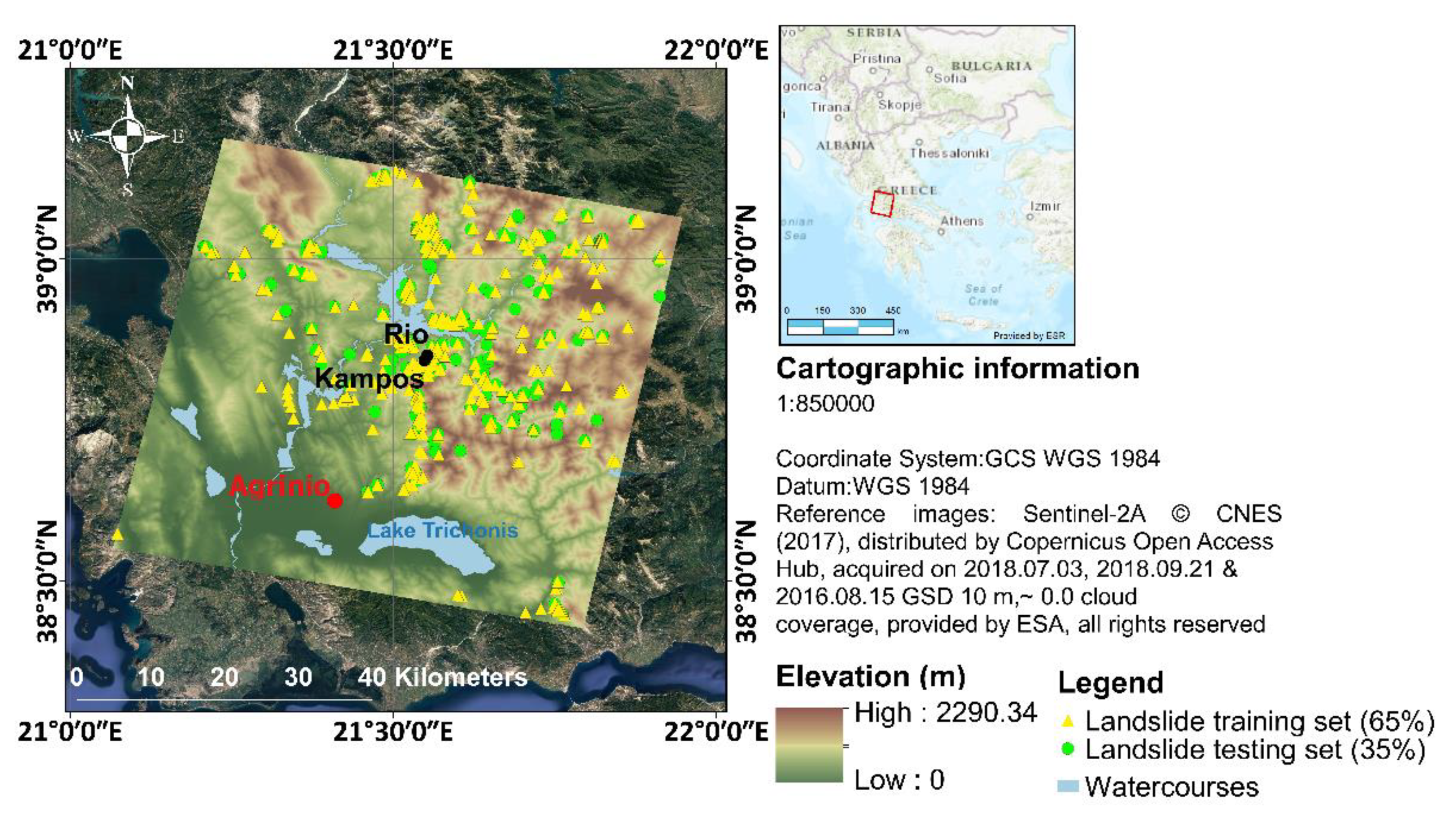
The consistency of deformation pattern derived from InSAR analysis was verified through photo-interpretation on high-resolution optical imagery and field investigations. Active landslides detected by the MTI technique and characterized by LOS velocity values higher than 2 mm/y were integrated with existing in situ surveying records derived from IGME’s campaigns. The inventory of HSGME consisted of 397 landslides, and it was enriched by 245 locations derived by SAR, visual photo interpretation and field visits (see
Supplementary Material—Figures S2 and S3). The updated landslide inventory including 642 mapped events was finally taken into consideration to feed the statistical analysis of the landslide susceptibility. A training set corresponding to 65% of landslide events was used for the model simulation while the rest 35% was retained for the validation process (
Figure 7).
4.1.2. Inventory Validation (In-Field Visits and Visual Photo Interpretation)
In order to evaluate the success of landslide identification by SAR analysis, in-field visits, and visual photo interpretation were performed. MTI technique has successfully resulted in the identification of past slope failures and the detection of new, active very slow to slow-moving landslides. It should be pointed out that MTI technique limits the identification of surface deformations along the LOS direction. In our analysis, the use of data sets acquired in LOS descending geometry allowed the detection of ground movements only in the vertical direction. For this reason, the integration of ascending and descending data should be used in order to retrieve ground deformations in all possible slope orientations. Moreover, it should be pointed out that the MTI technique cannot provide information for fast moving slides that may even take place between successive acquisitions. In that case, other techniques, such as visual photo interpretation, should be applied.
A significant contribution of MTI analysis is that the landslides could be detected in remote mountainous areas where the field investigation was difficult or, in some cases, infeasible to do. It should be noted that inherent characteristics of the landslides, such as color, high contrast, size, and shape (i.e., spoon-like rupture surfaces) were taken into consideration as indicator parameters for the landslide identification at a more detailed level. As an example,
Figure 8 presents extensive active debris flows threatening Kampos and Rio villages. The unstable slopes are made up by intensively fractured platy limestone and radiolarites (chert-like formations) of the Pindos Zone. According to the MTI analysis, the ground deformation LOS velocity values range from 5 up to 11 mm/y, with the maximum values occurring at the steeper parts of the slopes.
Landslide phenomena were also reported as threats of residential areas, as in the cases of Peristeri village. The village is founded on intensively fractured rock formations of the Pindos geotectonic zone composed of thin platy limestone, in alteration with chert and shale formations, upthrusted by shale and chert formations. This geological environment is susceptible for the manifestation several failure mechanisms, such as rotational slides or debris flows. The distribution of the PSs indicate that the central part of the village is affected by a rotational slide (
Figure 9) moving with LOS velocities ranging from 3 to 6 mm/y. Moreover, the northwestern side of the village, along the crest of the slope, is affected by a small debris flow expanding with LOS velocities of 2 to 3 mm/y. Both failure mechanisms have been verified by the field visits.
4.2. Weights of Evidence for Landslide Susceptibility Modeling
Weights of evidence is a statistical method initially developed for medical diagnosis purposes. In the late 1980 s, it was expanded in spatial applications for mineral potential mapping [
57,
58]. It is based on spatial correlation between past events and predisposing factors in order to determine patterns of high probability occurrences. A positive weight (W
+) due to the presence of events and a negative weight (W
−) due to the absence of the events are calculated for each factor. According to Bonham-Carter et al. [
58], the weights for the
jth pattern are determined from the following equations:
where
bj is the number of unit cells where the pattern is present and
where the pattern is not present and d the unit cells.
Significant statistical parameters are the contrast (
C) and the studentized contrast (
St. C). The contrast,
, reflects the overall correlation between the pattern and the past events. It is used as an indicator to decompose which patterns are to be kept as unique categories and which are the ones that should be aggregated with others. The studentized contrast is the ratio of the contrast to the standard deviation of its underlying weights (
), [
59]. “A pattern can be considered a useful predictor for future occurrences when it has a large positive contrast, and its studentized contrast is also sufficiently large”, as reported by Brian [
60].
Weights of evidence method is implemented in two steps (
Figure 5, block B), the first being to calculate the weights, while the second is for the calculation of the response, using as input evidential maps (spatial data correlated with landslides), and reliably determined training points (landslide events). All evidential data are used in raster format in categorical classes, while the training points are in vector format. At the first step, tables were produced for each evidential layer displaying the statistical parameters (positive and negative weight, contrast, studentized contrast) for each class. In the following, these tables are used for the selection of the appropriate most influential layers and further for the reclassification of the layers in order to optimize predictor layers, maximize the contrast, and keep the studentized contrast parameter within an acceptable range. The method is not a “black box” procedure, as expert knowledge is needed for influencing the modeling in the reclassification process. At the second step, the predicted probability after considering the evidence is calculated.
Weights of Evidence Method Application and Results
All evidential layers including slope, aspect, curvature, length-slope (LS) factor, precipitation, faults, and geological formations were classified into multiple categories. Porwal et al. [
61] found that multi-class than binary reclassified evidential layers may result in better prediction rates and more finely differentiated posterior probabilities. Based on Bayesian statistics, weights were calculated in order to define the strength of spatial association between the landslide training set and the classes of each evidential layer (
Tables S1–S8). In the calculated weight tables, the statistical parameters, the area (in km
2), the GEN_CLASS value, and the number of landslide occurrences are given for each pattern of the evidential themes.
The GEN_CLASS value is returned by the model in order to indicate which patterns of the evidential layers should be integrated, as the confidence criteria are not sufficiently met. For these specific areas, the GEN_CLASS value is set to 99, indicating the generalization of this specific class. Acceptable classes are given a GEN CLASS value, which is equal to the value in the evidence.
Calculate weights tool requires also two parameters, the unit area, and the confidence level of studentized contrast. One assumption of weights of evidence modeling is that there is only one training point per unit cell [
62]. The unit area is used as the counting unit for area measurements in the weights of evidence. In the Response theme, the posterior probability will be the probability of a unit cell containing a training point. Weight values are relatively insensitive to unit cell size if unit cell is small [
63]. In our analysis, unit area value is determined by the mean landslide extension exploiting measurements of landslide occurrences in the study area. Thus, the unit area is assigned a value of 0.06 km
2. The confidence level defines an acceptable contrast. This measure is an approximate Student T test of the hypothesis that the contrast is not zero. Confidence level is kept in default level of value equal to 2.0, which indicated approximately 98% confidence.
Slope, faults, and curvature evidential themes are not reclassified as all classes have high contrast or high confidence level of studentized contrast. The rest evidential themes are reclassified in order to achieve maximum contrast and simultaneously to keep studentized contrast values within an acceptable range (
Tables S9–S13). The reclassified evidence maps are finally combined to generate the continuous-scale posterior probability map. Several screenshots of the reclassified layers are shown in
Figure 10.
Several iterations are conducted in order to investigate the influence of each evidential layer in the susceptibility map (
Table 2). Test results using different combinations of evidential maps (predisposing factors) are presented in the following table. The performance of the model is improved using more evidential layers as proved by success rate of the various iterations. Success and predict rates (compatibility and predictability) are generated by the area–frequency table tool in ArcSDM. Success and prediction rate difference is less than 15% indicating reliable good quality of the model. The performance of the statistical model is evaluated using areas under curve (AUC) [
64]. The success rate is calculated by comparing the training set with the susceptibility map. The predictive rate was generated using the validation set which was not used to build the model. The success rate describes how well the model fits with past landslide occurrences and prediction rate describes how well the model predicts the landslide occurrence in the future.
Evaluating the success and prediction rate values presented in
Table 2 it is clear that main predisposing factors are those describing the geology (geology and faults) and the morphology (slope and aspect), succeeding 76.4 and 75.2 success and prediction rate values, respectively. The rest of the factors contribute by further increasing the accuracy of the produced susceptibility map.
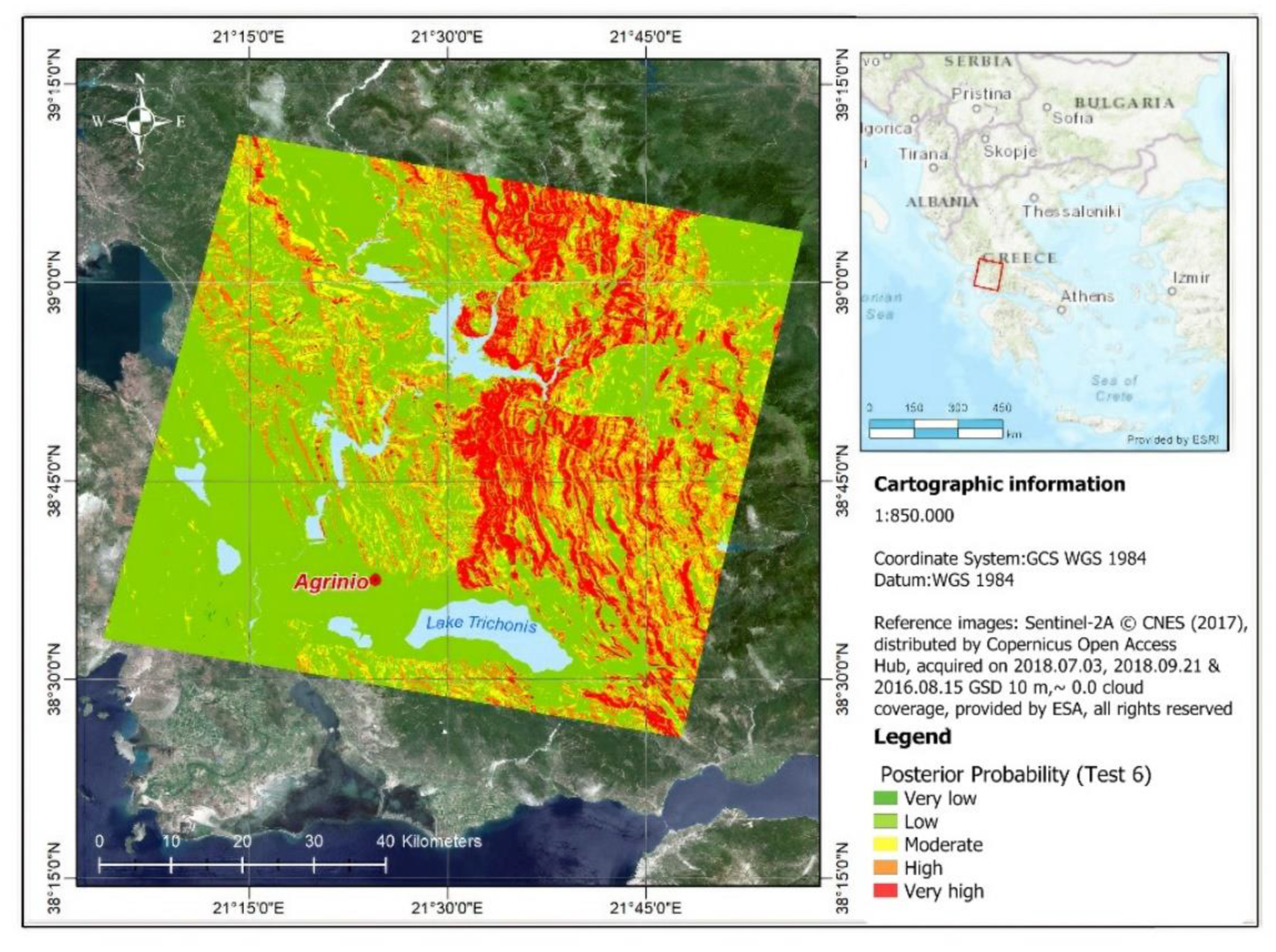
Figure 11 presents the landslide susceptibility map referring to tests 1 and 6. Comparing the two results, it is obvious that adding appropriate predisposing factors in the modeling process leads to greater success and prediction rate, as well as better illustration of the different susceptibility classes.
4.3. Norwegian Geotechnical Institute (NGI) Method for Landslide Susceptibility Modeling
The NGI is a generic method used in the Global Risk Update (GRU) study of UNISDR [
65] and in Global Assessment Report 2013 (GAR 2013) [
66]. It is a modified version of the approach used by Nadim et al., 2006, 2012 [
67,
68], to identify global landslide hazard and risk “hotspots”, based on the proposed procedure by Mora and Vahrson [
69]. The method defines the landslide susceptibility as the annual probability of landslide occurrence estimated by an appropriate combination of the triggering factor (rainfall) along with susceptibility factors (
Figure 5, block C).
The landslide susceptibility index due to rainfall is estimated using the following equation [
69]:
where S
r is the slope factor within a selected grid, S
l is the lithological (or geological) conditions factor, S
h describes the soil moisture condition, S
v describes the vegetation cover, and T
p is the precipitation factor.
The slope factor is calculated by EU-DEM and the vegetation coverage estimated by CLC, as in the statistical method. The soil moisture conditions index does not taken into consideration due to low resolution of moisture open data derived especially from Climate Prediction Center (CPC; Fan and Van den Dool [
70]) in conjunction with the small coverage of the study area.
The precipitation factor is based on the estimation of the 100-year extreme monthly rainfall exploiting monthly quasi-global rainfall dataset, derived from the Climate Hazards Group InfraRed Precipitation with Station open data (CHIRPS).
Regarding the geological conditions, EGDI (European Geological Data Infrastructure) 1:1 Million OneGeology pan-European Surface Geology map (
Figure 12) (
http://www.europe-geology.eu/, accessed on 17 March 2021) [
71], harvested from Infrastructure for Spatial Information in Europe (INSPIRE) conformant National Web Feature Services (WFS) on Geologic Unit (
https://inspire.ec.europa.eu/, accessed on 17 March 2021) [
72], was used.
By considering both lithology (
Figure 12a) and age (
Figure 12b), the lithology factor, S
l, was selected and introduced at the NGI model. As indicated at
Table S2, of the supplementary material, by applying the weight values suggested by Nadim et al. [
67], the formations of the study area belong to the same susceptibility classes regardless of the criterion used for their classification, lithology, or age.
Weight values are assigned to the classes of the susceptibility and triggering factors, taking into consideration a conceptually consistent physical basis. These weight values are confirmed from tables presented in Nadim et al. [
67], which relate the weight values of factors with specific characteristics (see
Supplementary Material—Tables S14–S18). Rainfall-induced landslide susceptibility hazard map based on the applied NGI method is presented in
Figure 13.
5. Discussion
Through the WoE method, several results for the predisposing factors came up, taking into account the statistical parameters of the model. High values on contrast and studentized parameters for specific patterns of the predisposing factor indicate the areas with high probability of landslide occurrences.
According to the WoE results, high probability of landslide occurrences appears where the aspect is of southwest and west orientation. The aspect of a slope influence indirectly the landslide occurrence because it controls the exposition of the slopes to climate conditions (duration of sunlight exposition, precipitation intensity, moisture retention, etc.), and as a result their vegetation cover [
73,
74,
75,
76,
77,
78]. Based on the hydrometeorological conditions of the study area, the southwest and west oriented slopes are more violently affected by rainfalls.
Both slope and length–slope factor have similar statistical behavior. As the factor values increase, the contrast values increase, respectively, indicating that the increased values are correlated with high probability of landslide occurrences. Slope angle and geometry are controlling factors in slope stability. When dealing with soil or intensively fractured rock formations stability issues occur when slope angle exceeds the friction angle of the geomaterials. Respectively, when dealing with rock formations, the steeper and the higher the slopes, the larger the amount of rock wedges exposed on the slope faces.
An expected conclusion is that higher contrast values correspond to concave terrain as well as areas within the fault zones. This is justified by the fact that old landslides have a concave geometry and occur close to upthrust and overthrust faults. Moreover, in concave terrain, surface water tends to run towards the area, increasing the saturation of soils, thus altering the geotechnical properties of the geo-materials triggers landslide initiation.
Artificial surfaces and agricultural areas have the highest contrast and large studentized contrast values compared with the other land use categories. Slope failures induced in these land use categories due to the disturbance by human activities, such as slope changes in agricultural areas or road construction in prone mountainous areas. Moreover, in agricultural areas, ground water level changes and saturation of geomaterials tend to activate failures either due to the fluctuation of the water pore procure or due to the degradation of the mechanical properties of the rock materials.
Through the statistical model, it is concluded that rainfall values of 120–160 mm per day for 50 years return period (high probability of appearance) relate to more susceptible areas.
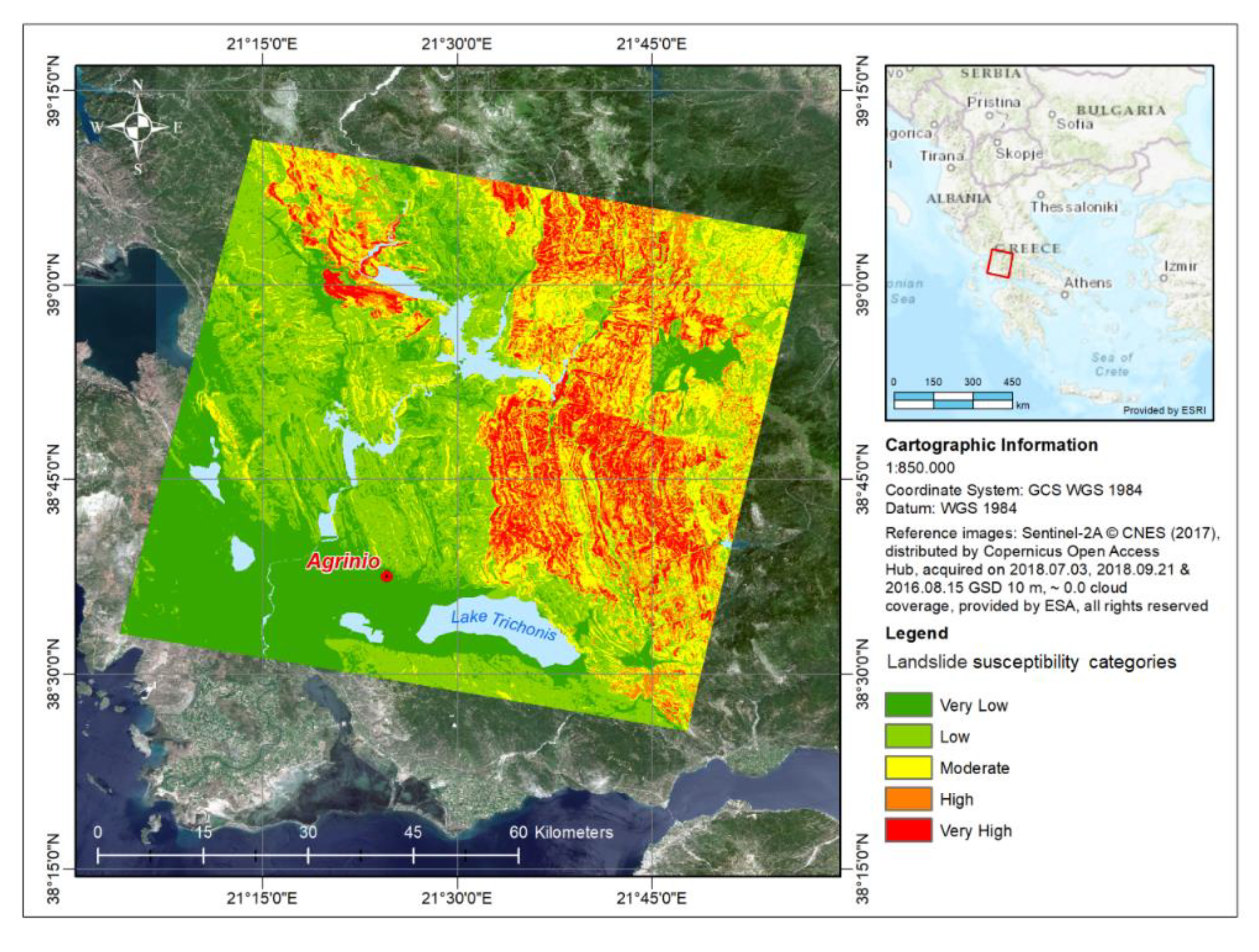
Considering all the iterations for probability map, it was concluded that landslide susceptibility map, derived from all predisposing factors (test 6), including slope, faults, geology, aspect, Corine land cover, LS factor, and precipitation T = 50 years, shows that the highest success rate and prediction rate corresponded to 80.8% and 79.5%, respectively.
On the other hand, the landslide susceptibility map due to rainfall, provided through the NGI methodology, exhibits several inconsistencies and misfits. In particular, several geospatial data are not taken under consideration such as the major tectonic lines (trust and fault zones), the aspect of the slopes and primarily the landslide inventory. Furthermore, by combining geospatial data from different scales, it results in providing maps dominated by scale effects.
Aiming to compare the maps produced by the two methodologies, a map indicating the difference of landslide susceptibility level between the WoE (test 6) and the NGI has been produced (
Figure 14). Reviewing the distribution of the purple shading sites, it is clear that several areas rated with higher landslide susceptibility index by the NGI method can be identified. The fact is that most of them are practically areas with much lower landslide susceptibility. For instance, the two areas surrounded by the circles refer to slopes with much gentler inclination than the surrounding slopes and, furthermore, to slopes with not any reported past landslide events. On the contrary, the green colored strips (pointed by the arrows) refer to the major trust zones, affecting mainly the formations of the Pindos geotectonic zone. The high landslide susceptibility of those areas is totally ignored by the NGI approach.
Thus, it is clear that by introducing small-scale open-source data sets as well as by disregarding several important predisposing factors, the accuracy of the NGI landslide susceptibility maps downgrades. On the other hand, the NGI methodology identified successfully the main distribution of the highly susceptible areas at the Pindos geotectonic zone by applying a fast procedure requiring low accuracy data.
It is worth mentioning that the landslide inventories, derived from either in situ observations or InSAR analysis, are biased, as they are strongly related to the land use and land cover classes. The in-situ based landslide inventory includes failures, located either mostly in the vicinity of residential areas or along roads and rail networks. On the other hand, the InSAR derived inventories tend to include landslides concentrated in artificial areas or non-vegetated areas. To be able to fill in the gap and obtain a more complete assessment for the occurring landslides, one would consider using low-cost corner reflectors thus enabling InSAR based inventories to be reported also in forested and agricultural areas.
An important scientific interest for further investigation is the correlation between rainfall and slope instability phenomena. In the literature, several studies have been conducted with the aim of proposing rainfall thresholds, empirical [
79,
80,
81] or physical [
82,
83], for the initiation of landslides. Determination of rainfall thresholds is a complex procedure, which depends on the, (i) threshold type (e.g., intensity, total rainfall amount); (ii) landslide type (e.g., shallow or deep-seated landslide); (iii) precedent rainfall conditions (e.g., saturated soil); and (iv) scale of the study (e.g., global, regional, or local). InSAR landslides inventories added slow moving landslides in the existing inventory of slow and fast moving events. An interesting aspect, that is worth investigating and will be integrated in future work, will be the influence of a balanced inventory in the validation process of the susceptibility map. Regarding the impact of a high-resolution DEM on the generation of geomorphometric parameters, DEMs of different accuracy could be employed and the impact of slope and aspect accuracy in the landslide susceptibility as assessment could be worth investigating in future analysis. An operational landslide early warning system, considering rainfall thresholds, can be used as a supporting tool for risk preparedness and mitigation actions [
84,
85].
At this final part of the discussion, we focus on the value of the susceptibility maps and the views of geoscientists, represented in this paper by HSGME. The expert’s opinion, which is necessary to reliably influencing the modeling outputs, is constantly integrated in the process, e.g., in the grouping of geological formations to the expected geo-mechanical behaviors, or to selecting the most appropriate factors influencing the landslide manifestation. Moreover, a-priori of the landslide mechanism helps the introduction of buffer zones, where both the surface and footwall formations are known.
6. Conclusions
The landslide susceptibility product derived from WoE method benefited from two main advantages, which are the expert opinion and the landslide inventory. This makes the method more reliable, realistic, and accurate. An innovative element of the study refers to the integration of massive InSAR observations, covering almost two decades from 1992 to 2010. This has significantly enriched the existing inventory of the known landslides in the study area. It is also important to highlight that, before this study was conducted, the reported landslides were located mostly nearby the villages and roads of the study area. Very little (almost zero knowledge) existed for the dominating mountainous sites, which show the highest risk levels for land sliding. Innovation lies also with the fact that the tectonic (faults) and geological elements of the area were used in the study and resulted in being representative of the main predisposing factors, complementing the usual morphological parameters used so far in similar studies, namely slope and aspect. One drawback of the method is the time-consuming processes required, due to the iterative “calculate weighted” process. However, the main and basic drawback is linked with the need for integrating a-priori knowledge for the area derived from exhaustive inventories of past events. The latter is considered the main disadvantage, which, as shown, could be addressed, to a good extent, by integrating InSAR calculations of slowly moving slopes over the past decades.
On the other hand, the NGI methodology, although less accurate, can be implemented immediately with minimum data and time requirements. It is more generic integrating less and easily discoverable knowledge for the studied area. Moreover, as shown in
Figure 14, the resulting susceptibility map, although less accurate compared to the WoE results, is still acceptable providing comparable results. Moreover, the higher residuals, located as green and purple segments in
Figure 14, could be investigated and resolved, to a good extent, by the expert’s opinion, in a post analysis and interpretation study of the results. This important outcome was key in the decision of the authors to use the NGI technique as a good approximation in the framework of several Copernicus Emergency Management Service (EMS) activations for Risk and Recovery. Indeed, in these activations, we have been requested, very often, to return, in a very short time frame, the assessment of landslide risks in completely unknown areas over the globe, using limited input data, the latter in the usual case being global scale data sets. However, as the method combines geospatial global data from different scales, it results in getting maps dominated by scale effects, as shown herein. This decreases the level of reliability in the assessments, but only when large-scale studies with local specificities are concerned.
In conclusion, we would like to stress that the expected use of the produced susceptibility maps influence the selected scale–accuracy and the appropriate methodology, and vice versa.
Small-scale maps (≤100,000) are suitable only for a general use; they can be used at European or national levels, and they help politicians and decision makers quantify the problem of landslides. Medium scale susceptibility maps (1:25,000) are crucial for the initial design of infrastructure and lifelines, while large-scale maps (1:5000 to 1:500) are suitable for urban development and the final design of infrastructure, large technical works, and lifelines.
In any case, these methodologies are efficient for small or medium landslide susceptibility modeling used at the draft design stage of an infrastructure project before the detailed design.


 ,
, 


