Almost-Minimal-Round BBB-Secure Tweakable Key-Alternating Feistel Block Cipher

Abstract

This paper focuses on designing a tweakable block cipher via by tweaking the Key-Alternating Feistel ($\mathsf{KAF}$ for short) construction. Very recently Yan et al. published a tweakable $\mathsf{KAF}$ construction. It provides a birthday-bound security with 4 rounds and Beyond-Birthday-Bound (BBB for short) security with 10 rounds. Following their work, we further reduce the number of rounds in order to improve the efficiency while preserving the same level of security bound. More specifically, we rigorously prove that 6-round tweakable $\mathsf{KAF}$ cipher is BBB- secure. The main technical contribution is presenting a more refined security proof framework, which makes significant efforts to deal with several subtle and complicated sub-events. Note that Yan et al. showed that 4-round $\mathsf{KAF}$ provides exactly Birthday-Bound security by a concrete attack. Thus, 6 rounds are (almost) minimal rounds to achieve BBB security for tweakable $\mathsf{KAF}$ construction.

1. Introduction

A block cipher, also known as a pseudorandom permutation, which is a pair of algorithms $(E,D)$. A block cipher has two important parameters: block length and key length. If the block length is n bits and the key length is k bits, for a mathematical point of view, the block cipher can be seen as a mapping

$${\{0,1\}}^k\times {\{0,1\}}^n\to {\{0,1\}}^n.$$

E represents a mapping that from the key space and the message space to the message space, and D is the opposite direction of the mapping in E. In addition, we call E is encryption, and D is decryption. The schemes of block cipher are roughly separated into two main classes, which are named Feistel networks and substitution—permutation networks (SPNs).

The tweakable block cipher is formalized by Liskov et al. [1]. It introduces to the block cipher an extra public input parameter tweak. The tweak provides inherent variability for building higher higher-level cryptographic schemes, namely modes of operation. So far, the tweakable block cipher has got received wide applications. Examples include Message Encryption, Message Authentication Code [1,2], and Authenticated Encryption Mode [3,4,5], etc. Now designing secure tweakable block ciphers has become a very important research topic. Cryptographers build tweakable block ciphers either from the scratch [6,7,8], or based on existing cryptographic primitives such as block ciphers or permutations [2,9,10,11]. Among these approaches, one is introducing the tweak to general structures of classical block ciphers, namely the Feistel construction [12] and the Even—Mansour construction [13]. We refer the interested readers to [9,14,15,16,17,18] for tweaking the Even—Mansour construction.

This paper mainly focuses on tweaking the Feistel construction. Since invented by Horst Feistel in 1973 [12], the Feistel construction has been a mainstream class of block ciphers. More specifically, there are several Feistel construction variants, such as Luby—Rackoff [19], Generalized Feistel [20], Key-Alternating Feistel [21], etc. They have been adopted in dedicated block ciphers including international and national standards. In 2007, Goldenberg et al. published the first paper of incorporating tweak to the Feistel constructions [22]. In particular, they paid attention to the Luby—Rackoff ciphers, and XOR tweaks to the dataflow branches. We write such tweak injection as linear tweak injection in this paper. Goldenberg et al. found that 6 rounds and more are secure (against polynomial adversaries). Moreover, they showed that 10 rounds are secure against $2^n$ adversarial queries, that is i.e., fully secure with n as the branch bit size of Luby—Rackoff structure. After that, Mitsuda and Iwata analyzed tweaking Generalized Feistel Structures with similar linear tweak injection [20]. They proved that $2d$ rounds are birthday-bound secure with d as the number of branches of Generalized Feistel Structure. Very recently, Yan et al. published a result of tweaking the Key-Alternating Feistel ($\mathsf{KAF}$) Cipher [23]. They introduced the tweak by mixing round keys, and proved that 4 rounds have a birthday-bound security and 10 rounds enable a beyond-birthday-bound security of roughly $2^{2n/3}$ adversarial queries with n as the branch bit size. We will carry on the research of tweaking the $\mathsf{KAF}$. (It is referred to as Feistel-2 in IACR Tikz Library).

The Feistel network [12] is a popular structure of block ciphers. In the i-th round of the Feistel cipher, the intermediate state of input $x_i=L\Vert R$ is updated by the round function $G_i$, i.e., $L\Vert R\to R\Vert L\oplus G_i(k_i,R)$. After tweaking the generalized Feistel ciphers by Mitsuda and Iwata [20], there is are only a few works about tweaking the Feistel cipher. The most mainstream research is tweaking $\mathsf{KAF}$ ciphers as Yan et al did recently [23]. They introduced the tweak with several round keys by using a universal hash function $H(·)$, that is, $t{k}_i\leftarrow H_{k_i}\left(t\right)$, where $k_i$ is the secret key, t is the tweak. By tweaking $\mathsf{KAF}$ with the i-th round function, the input is updated through

$$m_L\Vert m_R\leftarrow m_R\Vert m_L\oplus F_i(H_{k_i}\left(t\right)\oplus m_R),$$

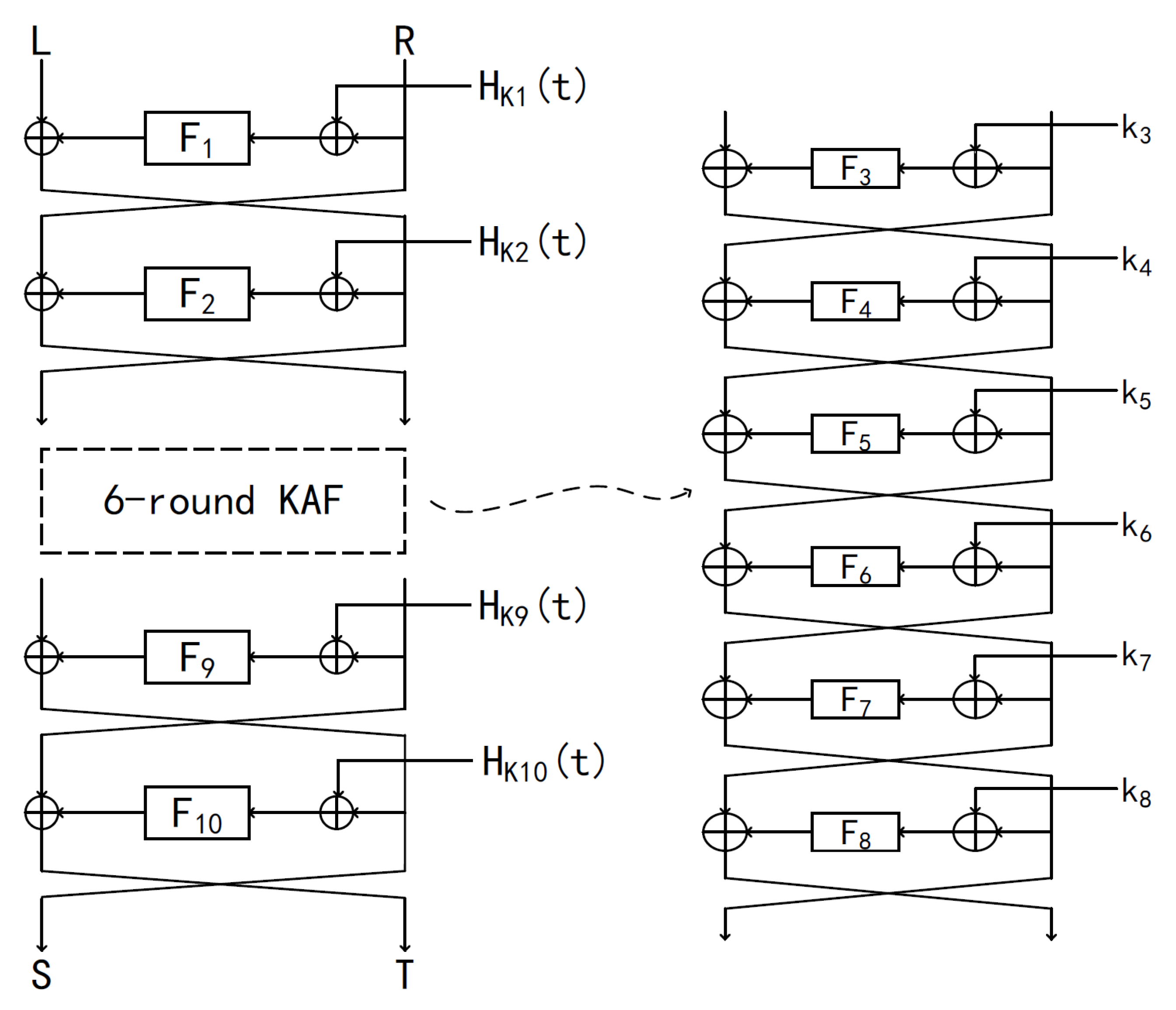
where $F(·)$ is the ith-round function. Yan et al. presented a 4-round minimized structure with two round keys and a single random function, proved that it achieves Birthday-Bound security. Meanwhile, they presented a 10-round tweakable $\mathsf{KAF}$ ($\mathsf{TKAF}$ for short) construction (depict in Figure 1) that can achieve BBB security. In this work, we aim to optimize Yan et al’s 10-round structure, and adopt other distinct construction of tweakable block ciphers. Then we give the proof that the new construction still meets the BBB security. We compared with Yan et al’s work [23] which lists in

Table 1. Comparison with related works.

Key Size	Rounds	Number of Round Functions	Bound	Reference
10n	10	10	2n/3	Yan et al. [23]
6n	6	6	2n/3	Guo et al. [24] (without tweak)
6n	6	6	2n/3	Section 3 (tweaked)

.

1.1. Our Contributions

In this paper, we present a 6-round $\mathsf{TKAF}$ cipher which meets the BBB security, with tweaking the additional outer four rounds based on based on Guo et al.’s 6-round $\mathsf{KAF}$ [24]. Unlike Yan et al.’s research, we adopt the approach of introducing tweak into the 6-round $\mathsf{KAF}$ directly. By utilizing Guo et al’s proof methodology, we introduce the tweak via using a universal hash function. We prove when the adversary makes distinct queries with different tweaks, due to the uniformity of the mentioned hash function, it still meets BBB security.

1.2. Structure of This Paper

Section 2 is the preliminaries of notations and definitions. Section 3 is the overview of proofs and core contribution. Section 4 is the proof of our conclusion. Section 5 is the future work.

2. Preliminaries

2.1. Notations and General Definitions

Let n denote a positive integer. Then $N=2^n$ and $\mathcal{N}={\{0,1\}}^n$. $\mathcal{F}\left(n\right)$ denotes the set of all functions mapping from $\mathcal{N}$ to $\mathcal{N}$. $\mathcal{P}\left(2n\right)$ denotes the set of all permutations in the range of ${\{0,1\}}^{2n}$. Let $\theta \left(s\right)$ be a random variable relying on one another random variable s. Then we denote by ${\mathbb{E}}_{s\backslash \mathcal{S}}\left[\theta \left(s\right)\right]$ the expectation of $\theta \left(s\right)$ taken over all $s\backslash \mathcal{S}$. For $X,Y\backslash \mathcal{N}$, denote $X\Vert Y$ or simply $XY$ as their concatenation.

2.1.1. Block Cipher

A block cipher is a family of permutations indexed by the secret key. It is denoted as $E:\mathcal{K}\times \mathcal{M}\to \mathcal{C}$, where $\mathcal{K}$ is the key space, $\mathcal{M}$ is the message space, and $\mathcal{C}$ is the ciphertext space. Hence for each $K\backslash \mathcal{K}$, $E(K,·)$ or simply $E_K(·)$ is a permutation from $\mathcal{M}$ to $\mathcal{C}$. In this paper, $\mathcal{M}=\mathcal{C}={\{0,1\}}^{2n}$.

2.1.2. Tweakable Block Cipher

A tweakable block cipher is a family of permutations indexed by the secret key and the public tweak. It is denoted as $\tilde{E}:\mathcal{K}\times \mathcal{T}\times \mathcal{M}\to \mathcal{C}$, where $\mathcal{K}$ is the key space, $\mathcal{T}$ is the tweak space, $\mathcal{M}$ is the message space, and $\mathcal{C}$ is the ciphertext space. Hence for each $K\backslash \mathcal{K}$ and each $T\backslash \mathcal{T}$, $E(K,T,·)$ or simply $E_{K,T}(·)$ is a permutation from $\mathcal{M}$ to $\mathcal{C}$. Similarly, $\mathcal{M}=\mathcal{C}={\{0,1\}}^{2n}$. We denote $\tilde{\Pi }(\mathcal{T},2n)$ as the set of all tweakable permutations with $\mathcal{M}=\mathcal{C}={\{0,1\}}^{2n}$.

2.1.3. Key-Alternating Feistel ($\mathsf{KAF}$) Cipher

A $\mathsf{KAF}$ is a block cipher with $\mathcal{M}=\mathcal{C}={\{0,1\}}^{2n}$. It has an iterative structure. The i-th round function has the form ${\Psi }_{k_i}^{\mathit{F}}(L\Vert R)=(R\Vert L\oplus {\mathit{F}}_i(R\oplus k_i))$, where L and R are the left half and the right half of the inputs respectively, $k_i$ is the i-th secret round key, and ${\mathit{F}}_i$ is the i-th public round function. We denote the r-round $\mathsf{KAF}$ with r public round functions $\mathit{F}=({\mathit{F}}_1,\dots ,{\mathit{F}}_r)$ in $\mathcal{F}\left(n\right)$ and a round-key vector $k=(k_1,\dots ,k_r)$ by

$${\mathsf{KAF}}_k^{\mathit{F}}(L\Vert R)={\Psi }_{k_r}^{{\mathit{F}}_r}\circ \dots \circ {\Psi }_{k_1}^{{\mathit{F}}_1}(L\Vert R).$$

2.1.4. Uniform AXU Hash Functions

A set of hash functions is denoted as $\mathcal{H}:\mathcal{K}\times \mathcal{T}\to \mathcal{N}$. For each key $k\backslash \mathcal{K}$, a keyed hash function $H(k,·)$ or simply $H_k(·)$ maps the tweak space $\mathcal{T}$ to $\mathcal{N}$. $\mathcal{H}$ is said to be uniform hash function if for any $t\backslash \mathcal{T}$ and $y\backslash \mathcal{N}$,

$$Pr\left[k\stackrel{\$}{\leftarrow }\mathcal{K}:H(k,t)=y\right]=2^{-n}.$$

Moreover, it is said to be $ϵ$-almost XOR-universal ($ϵ$-AXU) if for any $t,t^{\prime }\backslash \mathcal{T}$ with $t\ne t^{\prime }$ and any $y\backslash \mathcal{N}$,

$$Pr\left[k\stackrel{\$}{\leftarrow }\mathcal{K}:H_k\left(t\right)\oplus H_k\left(t^{\prime }\right)=y\right]\le ϵ.$$

2.2. Security Definitions

A distinguisher $\mathcal{D}$ can be thought as a fundamental attacker, and it can make queries to one (or more) “oracle” which can be the block ciphers or the random permutations. The advantage of a distinguisher $\mathcal{D}$ in distinguishing two oracles $\mathcal{O}$ and $\mathcal{Q}$ can be defined as:

$$\mathit{Adv}\left(\mathcal{D}\right)=|\mathrm{Pr}\left[{\mathcal{D}}^{\mathcal{O}}\to 1\right]-\mathrm{Pr}\left[{\mathcal{D}}^{\mathcal{Q}}\to 1\right]|.$$

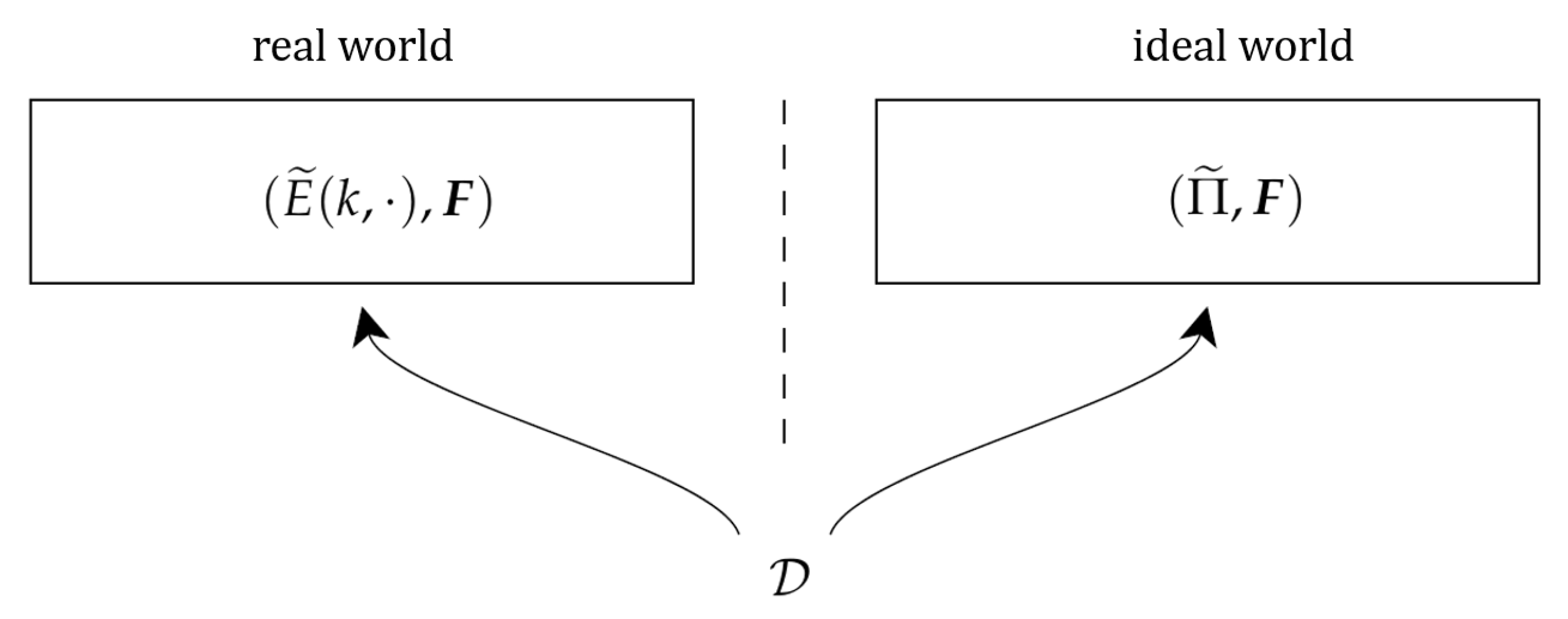
We discuss this under the Random Permutation model. Firstly, we define two worlds–“the real world” and “the ideal world”. When the distinguisher $\mathcal{D}$ interacts with the oracle $(\mathcal{O},\mathit{F})$, the real world means $\mathcal{O}$ is a tweakable block cipher $\tilde{E}(k,·)$, $\mathit{F}=(F_1,\dots ,F_r)$ is a public random function or permutation of $\tilde{E}$, where k is uniformly taken from $\mathcal{K}$. In addition, in the ideal world, $\mathcal{O}$ is a tweakable permutation $\tilde{\Pi }$ and $\mathit{F}=(F_1,\dots ,F_r)$ is a public random function or permutation of $\tilde{\Pi }$. We call $\mathcal{O}$construction oracle and $\mathit{F}$ inner component oracles. The security of a tweakable block cipher is measured by the advantage of the distinguisher $\mathcal{D}$ that distinguishes the two worlds: $(\tilde{E}(k,·),\mathit{F})$ and $(\tilde{\Pi },\mathit{F})$(depict in Figure 2). We write

$$\mathit{Adv}\left(\mathcal{D}\right)=|\mathrm{Pr}\left[{\mathcal{D}}^{\tilde{E}(k,·),\mathit{F}}\to 1\right]-\mathrm{Pr}\left[{\mathcal{D}}^{\tilde{\Pi },\mathit{F}}\to 1\right]|.$$

Theoretically, we only consider the information-theoretic distinguisher whose computation power is unlimited, i.e., it is determined, and only with limited information, that which means the number of access to the oracle is limited. We assume that the distinguishers do not make redundant queries. We also consider the distinguishers are under the chosen-ciphertext-attack (CCA) model, meanwhile they can choose tweaks, where they have the ability to query all the oracles either forward or backward.

We denote $q_e$ as the quantity of queries to the construction oracle and $q_f$ as the number of queries to each inner component oracle, then the definition of insecurity of the tweakable block cipher $\tilde{E}$ is

$${\mathit{Adv}}_{\tilde{E}}(q_e,q_f)=\underset{\mathcal{D}}{max}\left\{\mathit{Adv}\left(\mathcal{D}\right)\right\}.$$

H-Coefficient Technique

We utilizuse the H-coefficient technique [25,26] to evaluate the upper bound of the advantage of the adversary mentioned above.

Definition 1

(Transcript). A transcript $\tau =({\mathcal{Q}}_E,{\mathcal{Q}}_{\mathit{F}})$ is the response-tuple when the distinguisher $\mathcal{D}$ interacts with its oracle, where ${\mathcal{Q}}_E$ contains the tuples of the form $(t,LR,ST)\backslash \mathcal{T}\times {\{0,1\}}^{2n}\times {\{0,1\}}^{2n}$ which interacts with the construction oracle and ${\mathcal{Q}}_{\mathit{F}}$ contains the tuples $(x,y)$ which interacts with the inner component oracle.

By definition, we can see that $\mathcal{D}$ either makes the direct query $(t,LR)$ to the construction oracle with x to the inner component oracle, receiving answer $ST$ and y, or makes the inverse query $(t,ST)$ to the construction oracle with y to the inner component oracle, receiving answer $LR$ and x. Suppose that $|{\mathcal{Q}}_E|=q_e$, and there are m distinct tweaks in the ${\mathcal{Q}}_E$. We assume there exist $q_i(1\le i\le m)$ distinct queries for the i-th tweak, hence ${\sum }_{i=1}^m{q}_i=q_e$. That means ${\mathcal{Q}}_E=\bigcup {\mathcal{Q}}_{E_i},1\le i\le m$, where ${\mathcal{Q}}_{E_i}$ are the corresponding queries of the i-th tweak. Similarly, we have $|{\mathcal{Q}}_{F_j}|=q_f$ and ${\mathcal{Q}}_{\mathit{F}}=\bigcup {\mathcal{Q}}_{F_j},1\le j\le r$.

We note that all the transcripts of queries are directionless and disordered form, but according to our hypothesis that the distinguisher $\mathcal{D}$ is deterministic. Thus, there is a one-to-one mapping between this statement and the primitive transcript of the interaction of $\mathcal{D}$ with its oracles. Meanwhile, the output of $\mathcal{D}$ is a deterministic function of $\tau$.

In addition, for the function ${\mathit{F}}_j$ and its set of queries ${\mathcal{Q}}_{F_j}$, if for each $(x,y)\backslash {\mathcal{Q}}_{F_j}$, ${\mathit{F}}_j\left(x\right)=y$, we say that ${\mathit{F}}_j$extends${\mathcal{Q}}_{F_j}$, denoted by ${\mathit{F}}_j⊢{\mathcal{Q}}_{F_j}$. Similarly, for the permutation ${\mathit{P}}^{\left(i\right)}$ and its transcript sets ${\mathcal{Q}}_{E_i}$, if for each $(t,LR,ST)\backslash {\mathcal{Q}}_{E_i}$, ${\mathit{P}}^{\left(i\right)}(t,LR)=ST$, we say that ${\mathit{P}}^{\left(i\right)}$ extends ${\mathcal{Q}}_{E_i}$, denoted by ${\mathit{P}}^{\left(i\right)}⊢{\mathcal{Q}}_{E_i}$. With the above definition of “extend”, we can define ${\mathsf{KAF}}_{k^{\left(i\right)}}^{\mathit{F}}⊢{\mathcal{Q}}_{E_i}$. Finally, for ${\mathcal{Q}}_{\mathit{F}}=({\mathcal{Q}}_{F_1},\dots ,{\mathcal{Q}}_{F_t})$ and $\mathit{F}=({\mathit{F}}_1,\dots ,{\mathit{F}}_t)$, if ${\mathit{F}}_1⊢{\mathcal{Q}}_{F_1}\wedge \dots \wedge {\mathit{F}}_t⊢{\mathcal{Q}}_{F_t}$, then we have $\mathit{F}⊢{\mathcal{Q}}_{\mathit{F}}$.

We further define the probability that the interactions of the distinguisher $\mathcal{D}$ with the real world and the ideal world. In addition, we respectively denote them by ${\mathrm{Pr}}_{re}\left(\tau \right)$ and ${\mathrm{Pr}}_{id}\left(\tau \right)$, where $\tau$ is a transcript of these interactions.

With these definitions, we give the core lemma of the H-coefficient technique, and the distinguishing advantage could be inferred by the ratio of ${\mathrm{Pr}}_{re}\left(\tau \right)$ and ${\mathrm{Pr}}_{id}\left(\tau \right)$.

Lemma 1

(From [27]). Assume that there is a function $\phi (q_f,q_e)>0$ such that for every possible transcript τ with $q_e$ and $q_f$ queries of the two types it holds

$$|{\mathrm{Pr}}_{id}\left(\tau \right)-{\mathrm{Pr}}_{re}\left(\tau \right)|\le {\mathrm{Pr}}_{id}\left(\tau \right)·\phi (q_f,q_e),$$

then it holds

$${\mathit{Adv}}_{\mathsf{KAF}}(q_f,q_e)\le \phi (q_f,q_e).$$

According to [27], the upper bound of $|{\mathrm{Pr}}_{id}\left(\tau \right)-{\mathrm{Pr}}_{re}\left(\tau \right)|$ is named “$\phi$-point-wise proximity” of $\tau$, which was raised by Hoang and Tessaro (HT) [27]. We let $\mathcal{K}={\mathcal{K}}_{good}\cup {\mathcal{K}}_{bad}$, where ${\mathcal{K}}_{good}$ and ${\mathcal{K}}_{bad}$ are mutual exclusive subsets. Denote ${\mathrm{Pr}}_{re}(\tau ,k)$ as the probability that $\mathcal{D}$ interacts with the real world, where $k\backslash \mathcal{K}$, and ${\mathrm{Pr}}_{id}(\tau ,k)$ is that $\mathcal{D}$ interacts with the ideal world, where k is a “virtual” key uniformly selected from the key space $\mathcal{K}$. With the above definition, HT provided a lemma to establish point-wise proximity.

Lemma 2

(Lemma 1 of [27]). Fix a transcript τ with ${\mathrm{Pr}}_{id}\left(\tau \right)>0$. Assume that: (i) $\mathrm{Pr}\left[k\backslash {\mathcal{K}}_{bad}\right]\le \delta$, and (ii) there is a function $g:\mathcal{K}\to \left[0,\infty \right)$ such that for all $k\backslash {\mathcal{K}}_{good}$, it holds $\frac{{\mathrm{Pr}}_{re}(\tau ,k)}{{\mathrm{Pr}}_{id}(\tau ,k)}\ge 1-g\left(k\right)$. Then we have

$${\mathrm{Pr}}_{id}\left(\tau \right)-{\mathrm{Pr}}_{re}\left(\tau \right)\le {\mathrm{Pr}}_{id}\left(\tau \right)·(\delta +{\mathbb{E}}_{k\backslash \mathcal{K}}\left[g\left(k\right)\right]).$$

3. Overview

3.1. Beyond Birthday-Bound Security for Six Rounds

In the beginning, we need to guarantee that tweaking the $\mathsf{KAF}$ ciphers does not break its construction, and the influence on efficiency of the scheme execution can not cannot be enormous. For study of the execution efficiency and security, Liskov et al. [1] thought the cost of changing tweaks should be less than that of changing keys. However, the study by Jean et al. [14] showed that the adversary can hardly obtain the key, but has the ability to completely control the tweak.

In this paper, we use a nonlinear compound mode for tweaking the Feistel structure, instead of tweaking dependent or independent keys. As we known, the four rounds of $\mathsf{KAF}$ cipher do not meet BBB security [24], Yan’s [23] work showed that tweaking 10 rounds $\mathsf{KAF}$ cipher can meet BBB security. Our work shows a method for tweaking the $\mathsf{KAF}$ cipher by the nonlinear pattern, and reduces the rounds of the scheme. For requirement of security, we consider to introduce the tweak with the round-key vectors by using a universal hash function.

Firstly, we use the suitable round-key vector which was defined by Guo [24]:

Definition 2

(Suitable Round-Key Vector for 6 Rounds [24]). A round-key vector $k=(k_1,k_2,k_3,k_4,k_5,k_6)$ is suitable if it satisfies the following conditions:

(i) 

$k_1,k_2,k_3,k_4,k_5,k_6$ are uniformly distributed in ${\{0,1\}}^n$;

(ii) 

for $(i,j)\backslash \left\{\right(1,2),(2,3),(4,5),(5,6),(1,6\left)\right\}$, $k_i$ and $k_j$ are independent.

Yan’s [23] work used the minimized 6-round $\mathsf{KAF}$ as a “core”, with additional four more rounds on the first and last sides of the “core”, meanwhile introducing the tweak into these four rounds. They gave a 10-round $\mathsf{TKAF}$ construction with BBB security. In our work, we aim to“tweak” the first and last two rounds of the “core”, and use a universal hash function to merge the tweak into round-key vectors.

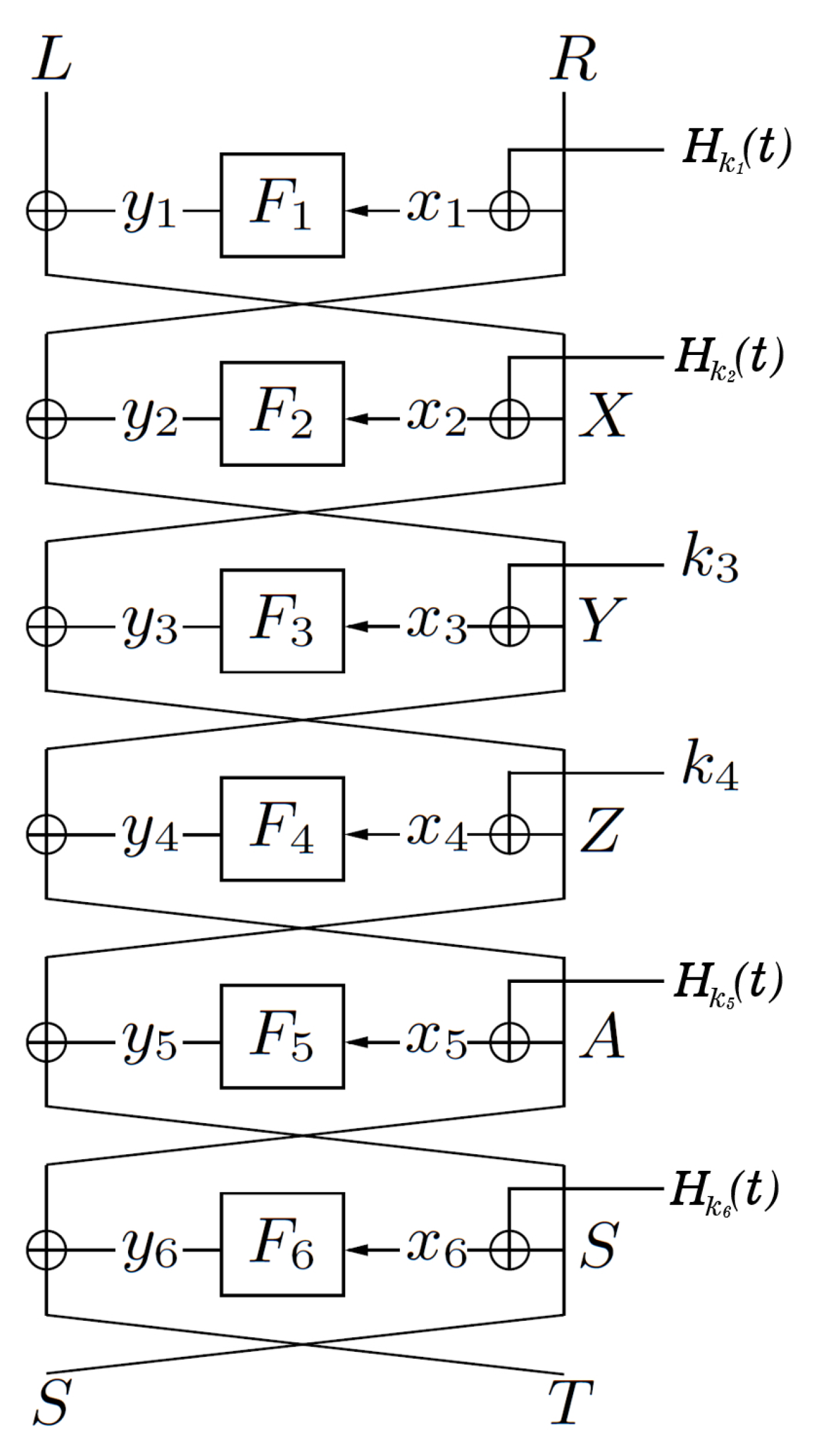
Next, we denote this 6-round construction by

$${\mathsf{TKAF}}_k^{\mathit{F}}(t,x)={\Psi }_{k_6,t}^{F_6}\circ {\Psi }_{k_5,t}^{F_5}\circ {\Psi }_{k_4}^{F_4}\circ {\Psi }_{k_3}^{F_3}\circ {\Psi }_{k_2,t}^{F_2}\circ {\Psi }_{k_1,t}^{F_1}\left(x\right),$$

where $\mathit{F}=(F_1,F_2,F_3,F_4,F_5,F_6)$ are random functions, $k=(k_1,k_2,k_3,k_4,k_5,k_6)$ are the corresponding round keys, $t\backslash \mathcal{T}$ is a tweak and $x\backslash {\{0,1\}}^{2n}$ is a message (depict in Figure 3).

Finally, we upper- bound the advantage of an adversary to attack this scheme. By utilizing the H-coefficient technique which is in Lemma 2, we firstly upper upper-bound the bad key event $\delta$, then upper- bound the expectation of the function $g\left(k\right)$, which holds $\frac{{\mathrm{Pr}}_{re}(\tau ,k)}{{\mathrm{Pr}}_{id}(\tau ,k)}\ge 1-g\left(k\right)$. By Lemma 1, we could obtain the advantage. Thus, we have this theorem:

Theorem 1.

For the 6-round tweakable $\mathsf{KAF}$ cipher with a suitable round-key vector as specified in Definition 2, it holds

$$\begin{array}{cc}\hfill {\mathit{Adv}}_{\mathsf{TKAF}}(q_f,q_e)& \le (7q_e^3+24q_e^2{q}_f+20q_e{q}_f^2)\frac{1}{N^2}\hfill \\ \hfill & +(4q_e^3+4q_e^2{q}_f+2q_e{q}_f^2+4q_e^2+6q_e{q}_f)\frac{\epsilon }{N}\hfill \\ \hfill & +4q_e^2{q}_f{\epsilon }^2+4q_e^2{\epsilon }^2.\hfill \end{array}$$

(1)

3.2. Core Contribution

In our work, we analyze the influence of tweaking $\mathsf{KAF}$ ciphers on security. We tweak the outer four rounds of Guo et al’s 6-round $\mathsf{KAF}$ and the proof of BBB security is the major research work we have done.

4. Security Proof of Theorem 1

In the following subsections, we present the methodology to prove Theorem 1. We fix a transcript $\tau =({\mathcal{Q}}_E,{\mathcal{Q}}_F)$ with ${\mathcal{Q}}_F=({\mathcal{Q}}_{F_1},{\mathcal{Q}}_{F_2},{\mathcal{Q}}_{F_3},{\mathcal{Q}}_{F_4},{\mathcal{Q}}_{F_5},{\mathcal{Q}}_{F_6})$, where $|{\mathcal{Q}}_E|=q_e$ and $|{\mathcal{Q}}_{F_i}|=q_f,i=1,\dots ,6$. We divide the analysis of this claim into two parts: $\left(i\right)$ define bad key vectors, then $\left(ii\right)$ lower bound the probability ${\mathrm{Pr}}_{re}(\tau ,k)$. We analyze these two parts respectively.

4.1. Bad Key Vectors and Probability

Definition 3

(Bad Key Vectors for 6 rounds). A suitable key vector $k\backslash \mathcal{K}$ is bad, for a transcript $\tau =({\mathcal{Q}}_E,{\mathcal{Q}}_F)$, if one of the follow conditions is met:

• (A-1)there exists $(t,LR,ST)\backslash {\mathcal{Q}}_E$, $(x_1,y_1)\backslash {\mathcal{Q}}_{F_1}$, $(x_6,y_6)\backslash {\mathcal{Q}}_{F_6}$, such that $H_{k_1}\left(t\right)=R\oplus x_1$, $H_{k_6}\left(t\right)=S\oplus x_6$;
• (A-2)there exists $(t,LR,ST)\backslash {\mathcal{Q}}_E$, $(x_1,y_1)\backslash {\mathcal{Q}}_{F_1}$, $(x_2,y_2)\backslash {\mathcal{Q}}_{F_2}$, such that $H_{k_1}\left(t\right)=R\oplus x_1$, $H_{k_2}\left(t\right)=L\oplus y_1\oplus x_2$;
• (A-3)there exists $(t,LR,ST)\backslash {\mathcal{Q}}_E$, $(x_5,y_5)\backslash {\mathcal{Q}}_{F_5}$, $(x_6,y_6)\backslash {\mathcal{Q}}_{F_6}$, such that $H_{k_6}\left(t\right)=S\oplus x_6$, $H_{k_5}\left(t\right)=T\oplus y_6\oplus x_5$.

otherwise, k is good. We denote ${\mathcal{K}}_{bad}$ for the set of bad key vectors, and ${\mathcal{K}}_{good}$ for the good key vectors.

In the beginning, we upper- bound the probability of the bad key vectors. Firstly, we analyze the above three conditions respectively, consider (A-1) first. Since we have the key $k_1$ and $k_6$ picked from the key space $\mathcal{K}$ uniformly and randomly, for the properties of suitable, $k_1$ and $k_6$ are independent of each other (Definition 2). By the uniformity of H, $H_{k_1}$ and $H_{k_6}$ are also independent. Thus Thus, there are $N^2$ possible choices. For $(t,LR,ST)\backslash {\mathcal{Q}}_E$, $(x_1,y_1)\backslash {\mathcal{Q}}_{F_1}$ and $(x_6,y_6)\backslash {\mathcal{Q}}_{F_6}$, we have at most $q_e{q}_f^2$ choices, as $|{\mathcal{Q}}_E|=q_e$, $|Dom{\mathcal{F}}_1|=|Dom{\mathcal{F}}_6|=q_f$, where $Dom\mathcal{F}$ is a set of x that there exists $(x,y)\backslash {\mathcal{Q}}_F$ such that $F\left(x\right)=y$, i.e., $Dom\mathcal{F}\stackrel{def}{=}\{x\backslash {\{0,1\}}^n:\exists (x,y)\backslash {\mathcal{Q}}_F,F\left(x\right)=y\}$. Therefore, the probability of condition (A-1) is at most $\frac{q_e{q}_f^2}{N^2}$.

Similarly, by definition of suitable key vector (Definition 2), it also holds that $(k_1,k_2)$, $(k_5,k_6)$ are independent, and for the uniformity of H, we have $\mathrm{Pr}\left[\left(\mathbf{A-2}\right)\right]=\mathrm{Pr}\left[\left(\mathbf{A-3}\right)\right]\le \frac{q_e{q}_f^2}{N^2}.$

To sum up, we can upper- bound the probability of the bad key vectors with

$$\mathrm{Pr}\left[k\stackrel{\$}{\leftarrow }\mathcal{K}:k\backslash {\mathcal{K}}_{bad}\right]\le \frac{3q_e{q}_f^2}{N^2}.$$

(2)

4.2. Analysis for Good Keys

In the following, we fix the round- key vectors $k\backslash {\mathcal{K}}_{good}$, and aim to lower bound the probability $\mathrm{Pr}\left[\mathit{F}\stackrel{\$}{\leftarrow }{\left(\mathcal{F}\left(n\right)\right)}^6:{\mathsf{TKAF}}_k^{\mathit{F}}⊢{\mathcal{Q}}_E|\mathit{F}⊢{\mathcal{Q}}_F\right]$. By the analytical method of Cogliati et al. [9,15], we divide this proof process into two steps: $\left(i\right)$ upper bounding the probability that a pair of functions $({\mathit{F}}_1,{\mathit{F}}_6)$ satisfies “bad” conditions. By these means, the “good” conditions of the function -pair can transfer the transcripts of the distinguisher on 6 rounds to a special transcripts on 4 rounds, it can be said that we “peel off” the outer two rounds [24]; then $\left(ii\right)$ assuming that $({\mathit{F}}_1,{\mathit{F}}_6)$ is good, by bounding the inner 4 rounds, we will prove the claim of Theorem 1.

Peeling Off the Outer Two Rounds

We pick a pair of round functions $({\mathit{F}}_1,{\mathit{F}}_6)$ such that ${\mathit{F}}_1⊢{\mathcal{Q}}_{F_1}$ and ${\mathit{F}}_6⊢{\mathcal{Q}}_{F_6}$. For each transcript $(t,LR,ST)\backslash {\mathcal{Q}}_E$, denote $X\leftarrow L\oplus {\mathit{F}}_1(H_{k_1}\left(t\right)\oplus R)$ and $A\leftarrow T\oplus {\mathit{F}}_6(H_{k_6}\left(t\right)\oplus S)$. From this, we obtain $q_e$ transcripts with the form of $(t,RX,AS)$. For convenience, we denote a new set including all these introduced transcript tuples by ${\mathcal{Q}}_E^{*}({\mathit{F}}_1,{\mathit{F}}_6)$. Furthermore, we define two subsets of ${\mathcal{Q}}_E^{*}({\mathit{F}}_1,{\mathit{F}}_6)$, the transcripts that collide at the positions of X and A, respectively. Denote them by $\mathcal{ID}\left(X\right)$ and $\mathcal{ID}\left(A\right)$:

$$\begin{array}{cc}\hfill \mathcal{ID}\left(X\right)& =\{(t,RX,AS):(t,RX,AS)\backslash {\mathcal{Q}}_E^{*}({\mathit{F}}_1,{\mathit{F}}_6),Xisidentical\}\hfill \\ \hfill \mathcal{ID}\left(A\right)& =\{(t,RX,AS):(t,RX,AS)\backslash {\mathcal{Q}}_E^{*}({\mathit{F}}_1,{\mathit{F}}_6),Aisidentical\}\hfill \end{array}$$

In order to characterize $\tau$, we define four key-dependent quantities:

$$\begin{array}{cc}\hfill n_{\left(1\right)}\left(k\right)& \stackrel{def}{=}\left|\{((t,LR,ST),(x_1,y_1))\backslash {\mathcal{Q}}_E\times {\mathcal{Q}}_{F_1}:H_{k_1}\left(t\right)=R\oplus x_1\}\right|\hfill \\ \hfill n_{\left(6\right)}\left(k\right)& \stackrel{def}{=}\left|\{((t,LR,ST),(x_6,y_6))\backslash {\mathcal{Q}}_E\times {\mathcal{Q}}_{F_6}:H_{k_6}\left(t\right)=S\oplus x_6\}\right|\hfill \\ \hfill n_{(2,3)}\left(k\right)& \stackrel{def}{=}\left|\{((t,LR,ST),(x_2,y_2),(x_3,y_3))\backslash {\mathcal{Q}}_E\times {\mathcal{Q}}_{F_2}\times {\mathcal{Q}}_{F_3}:k_3=R\oplus y_2\oplus x_3\}\right|\hfill \\ \hfill n_{(4,5)}\left(k\right)& \stackrel{def}{=}\left|\{((t,LR,ST),(x_4,y_4),(x_5,y_5))\backslash {\mathcal{Q}}_E\times {\mathcal{Q}}_{F_4}\times {\mathcal{Q}}_{F_5}:k_4=S\oplus y_5\oplus x_4\}\right|\hfill \end{array}$$

Now we define the “bad event” on the pair $({\mathit{F}}_1,{\mathit{F}}_6)$. If the corresponding set ${\mathcal{Q}}_E^{*}({\mathit{F}}_1,{\mathit{F}}_6)$ of the pair $({\mathit{F}}_1,{\mathit{F}}_6)$ fulfills one of the following “collision” conditions, we say that the predicate is bad, denoted by $\mathsf{Bad}({\mathit{F}}_1,{\mathit{F}}_6)$:

• (B-1) there exists $(t,RX,AS)\backslash {\mathcal{Q}}_E^{*}({\mathit{F}}_1,{\mathit{F}}_6)$, $(x_2,y_2)\backslash {\mathcal{Q}}_{F_2}$, $(x_5,y_5)\backslash {\mathcal{Q}}_{F_5}$, such that $H_{k_2}\left(t\right)=X\oplus x_2$, $H_{k_5}\left(t\right)=A\oplus x_5$;
• (B-2) there exists $(t,RX,AS)\backslash {\mathcal{Q}}_E^{*}({\mathit{F}}_1,{\mathit{F}}_6)$, $(x_2,y_2)\backslash {\mathcal{Q}}_{F_2}$, $(x_3,y_3)\backslash {\mathcal{Q}}_{F_3}$, such that $H_{k_2}\left(t\right)=X\oplus x_2$, $k_3=R\oplus y_2\oplus x_3$;
• (B-3) there exists $(t,RX,AS)\backslash {\mathcal{Q}}_E^{*}({\mathit{F}}_1,{\mathit{F}}_6)$, $(x_4,y_4)\backslash {\mathcal{Q}}_{F_4}$, $(x_5,y_5)\backslash {\mathcal{Q}}_{F_5}$, such that $H_{k_5}\left(t\right)=A\oplus x_5$, $k_4=S\oplus y_5\oplus x_4$;
• (B-4) there exist two distinct $(t,RX,AS),(t^{\prime },R^{\prime }{X}^{\prime },A^{\prime }{S}^{\prime })\backslash {\mathcal{Q}}_E^{*}({\mathit{F}}_1,{\mathit{F}}_6)$, $(x_2,y_2)\backslash {\mathcal{Q}}_{F_2}$, such that $X=X^{\prime }$ and $H_{k_2}\left(t\right)=X\oplus x_2$; or symmetrically two distinct $(t,RX,AS),(t^{\prime },R^{\prime }{X}^{\prime },A^{\prime }{S}^{\prime })\backslash {\mathcal{Q}}_E^{*}({\mathit{F}}_1,{\mathit{F}}_6)$, $(x_5,y_5)\backslash {\mathcal{Q}}_{F_5}$, such that $A=A^{\prime }$ and $H_{k_5}\left(t\right)=A\oplus x_5$;
• (B-5) there exist two distinct $(t,RX,AS),(t^{\prime },R^{\prime }{X}^{\prime },A^{\prime }{S}^{\prime })\backslash {\mathcal{Q}}_E^{*}({\mathit{F}}_1,{\mathit{F}}_6)$, $(x_2,y_2)\backslash {\mathcal{Q}}_{F_2}$, such that $A=A^{\prime }$ and $H_{k_2}\left(t\right)=X\oplus x_2$; or symmetrically two distinct $(t,RX,AS),(t^{\prime },R^{\prime }{X}^{\prime },A^{\prime }{S}^{\prime })\backslash {\mathcal{Q}}_E^{*}({\mathit{F}}_1,{\mathit{F}}_6)$, $(x_5,y_5)\backslash {\mathcal{Q}}_{F_5}$, such that $X=X^{\prime }$ and $H_{k_5}\left(t\right)=A\oplus x_5$;

If the predicate $\mathsf{Bad}({\mathit{F}}_1,{\mathit{F}}_6)$ does not hold, then we can deem that $({\mathit{F}}_1,{\mathit{F}}_6)$ is good. Now we bound the probability of $\mathsf{Bad}({\mathit{F}}_1,{\mathit{F}}_6)$.

Lemma 3.

It holds

$$\begin{array}{cc}\hfill & \mathrm{Pr}\left[\mathsf{Bad}({\mathit{F}}_1,{\mathit{F}}_6)|{\mathit{F}}_1⊢{\mathcal{Q}}_{F_1}\wedge {\mathit{F}}_6⊢{\mathcal{Q}}_{F_6}\right]\hfill \\ \hfill & \le \frac{4q_e^2{q}_f+q_e{q}_f^2}{N^2}+\frac{q_f(n_{\left(1\right)}\left(k\right)+n_{\left(6\right)}\left(k\right))}{N}\hfill \\ \hfill & +\frac{n_{(2,3)}\left(k\right)+n_{(4,5)}\left(k\right)}{N}+4q_e^2{q}_f{\epsilon }^2+q_f\epsilon (n_{\left(1\right)}\left(k\right)+n_{\left(6\right)}\left(k\right)).\hfill \end{array}$$

Proof. 

We prove the above 5 cases of $\mathsf{Bad}({\mathit{F}}_1,{\mathit{F}}_6)$ on the condition of ${\mathit{F}}_1⊢{\mathcal{Q}}_{F_1}\wedge {\mathit{F}}_6⊢{\mathcal{Q}}_{F_6}$:

(B-1) For arbitrary $(t,RX,AS)\backslash {\mathcal{Q}}_E^{*}({\mathit{F}}_1,{\mathit{F}}_6)$, if there exists $(x_2,y_2)\backslash {\mathcal{Q}}_{F_2}$ and $(x_5,y_5)\backslash {\mathcal{Q}}_{F_5}$, such that $H_{k_2}\left(t\right)=X\oplus x_2$ and $H_{k_5}\left(t\right)=A\oplus x_5$. Then for the corresponding $(t,LR,ST)\backslash {\mathcal{Q}}_E$, we have $L\oplus {\mathit{F}}_1(H_{k_1}\left(t\right)\oplus R)=H_{k_2}\left(t\right)\oplus x_2$ and $T\oplus {\mathit{F}}_6(H_{k_6}\left(t\right)\oplus S)=H_{k_5}\left(t\right)\oplus x_5$. On account of the uniformity of H, it must hold $H_{k_1}\left(t\right)\oplus R\notin Dom{\mathcal{F}}_1$ (if $H_{k_1}\left(t\right)\oplus R\backslash Dom{\mathcal{F}}_1$ and $H_{k_2}\left(t\right)=X\oplus x_2$, then the condition (A-2) is fulfilled). Similarly, it must be $H_{k_6}\left(t\right)\oplus S\notin Dom{\mathcal{F}}_6$. Thus, on the condition of ${\mathit{F}}_1⊢{\mathcal{Q}}_{F_1}\wedge {\mathit{F}}_6⊢{\mathcal{Q}}_{F_6}$, ${\mathit{F}}_1(H_{k_1}\left(t\right)\oplus R)$ and ${\mathit{F}}_6(H_{k_6}\left(t\right)\oplus S)$ keep uniform. SoSo, the probability of both $L\oplus {\mathit{F}}_1(H_{k_1}\left(t\right)\oplus R)=H_{k_2}\left(t\right)\oplus x_2$ and $T\oplus {\mathit{F}}_6(H_{k_6}\left(t\right)\oplus S)=H_{k_5}\left(t\right)\oplus x_5$ holding is at most $\frac{1}{N^2}$. AndIn addition, the choices of all 3-tuples $(t,LR,ST)$, $(x_2,y_2)$, $(x_5,y_5)$ do not exceed $q_e{q}_f^2$. Therefore, we have Pr[(B-1)] $\le \frac{q_e{q}_f^2}{N^2}$.

(B-2) and (B-3) We consider (B-2) firstly.

There exists a 3-tuple $((t,LRX,AST),(x_2,y_2),(x_3,y_3))$, such that the number of $k_3=R\oplus y_2\oplus x_3$ is $n_{(2,3)}\left(k\right)$, where $(t,LRX,AST)$ is a joint notation of $(t,LR,ST)$ and its corresponding induced X and A. Moreover, $H_{k_2}\left(t\right)=X\oplus x_2$ means $L\oplus {\mathit{F}}_1(H_{k_1}\left(t\right)\oplus R)=H_{k_2}\left(t\right)\oplus x_2$. When $H_{k_1}\left(t\right)\oplus R\backslash Dom{\mathcal{F}}_1$, then it can not cannot hold $L\oplus Img{F}_1(H_{k_1}\left(t\right)\oplus R)=H_{k_2}\left(t\right)\oplus x_2$, otherwise (A-2) is fulfilled. Furthermore Furthermore, when $H_{k_1}\left(t\right)\oplus R\notin Dom{\mathcal{F}}_1$, on the condition of ${\mathit{F}}_1⊢{\mathcal{Q}}_{F_1}$, then ${\mathit{F}}_1(H_{k_1}\left(t\right)\oplus R)$ keeps uniform. Meanwhile H also keeps uniform, thus we have the probability of $L\oplus {\mathit{F}}_1(H_{k_1}\left(t\right)\oplus R)=H_{k_2}\left(t\right)\oplus x_2$ is at most $\frac{1}{N}$. Therefore, Pr[(B-2)]$\le \frac{n_{(2,3)}\left(k\right)}{N}$. The condition (B-3) is symmetric with (B-2), so with the similar analysis, we have Pr[(B-3)]$\le \frac{n_{(4,5)}\left(k\right)}{N}$.

(B-4) For the given pair of distinct merged transcripts $(t,LRX,AST)$ and $(t^{\prime },L^{\prime }{R}^{\prime }{X}^{\prime },A^{\prime }{S}^{\prime }{T}^{\prime })$ together with $(x_2,y_2)\backslash {\mathcal{Q}}_{F_2}$, we discuss the cases in three conditions:

• Case 1: when $t\ne t^{\prime }$, if it holds $H_{k_1}\left(t\right)\oplus R=H_{k_1}\left(t^{\prime }\right)\oplus R^{\prime }$, i.e., for the $\epsilon$-$AUX$ property of H function, the probability of $H_{k_1}\left(t\right)\oplus H_{k_1}\left(t^{\prime }\right)=R\oplus R^{\prime }$ is at most $\epsilon$. If $H_{k_1}\left(t\right)\oplus R\ne H_{k_1}\left(t^{\prime }\right)\oplus R^{\prime }$, we note that $H_{k_1}\left(t\right)\oplus R\notin Dom{\mathcal{F}}_1$, $H_{k_1}\left(t^{\prime }\right)\oplus R^{\prime }\notin Dom{\mathcal{F}}_1$, otherwise (A-2) is fulfilled. Thus, on the condition of ${\mathit{F}}_1⊢{\mathcal{Q}}_{F_1}$, ${\mathit{F}}_1(H_{k_1}\left(t\right)\oplus R)$ and ${\mathit{F}}_1(H_{k_1}\left(t^{\prime }\right)\oplus R^{\prime })$ are independent with each other, also keep uniformly random. Then it holds $\mathrm{Pr}\left[{\mathit{F}}_1(H_{k_1}\left(t\right)\oplus R)=L\oplus L^{\prime }\oplus {\mathit{F}}_1(H_{k_1}\left(t^{\prime }\right)\oplus R^{\prime })\right]\le \epsilon +(1-\epsilon )\frac{1}{N}\le \epsilon +\frac{1}{N}$. Therefore, the probability of the collision at the position $H_{k_2}\left(t\right)\oplus X$ and $X=X^{\prime }$ is at most $(\epsilon +\frac{1}{N})\epsilon \le {\epsilon }^2+\frac{1}{N}\epsilon$.
• Case 2: if $t=t^{\prime }$ and $R\ne R^{\prime }$, for $X=X^{\prime }$, the probability of ${\mathit{F}}_1(H_{k_1}\left(t\right)\oplus R)\oplus L={\mathit{F}}_1(H_{k_1}\left(t^{\prime }\right)\oplus R^{\prime })\oplus L^{\prime }$ is at most $\frac{1}{N}$. AndIn addition, for $H_{k_2}\left(t\right)=X\oplus x_2$, the probability of $H_{k_2}\left(t\right)={\mathit{F}}_1(H_{k_1}\left(t\right)\oplus R)\oplus L\oplus x_2$ is at most $\frac{1}{N}$. For the property of H, we have the probability of the collision at the position X is at most $\frac{1}{N^2}$.
• Case 3: if $t=t^{\prime }$ and $R=R^{\prime }$ but $L\ne L^{\prime }$, it can not cannot be held that $X=X^{\prime }$ and $H_{k_2}\left(t\right)=X\oplus x_2$.

To sum up, the probability of “former” part of (B-4) can not cannot exceed ${\epsilon }^2+\frac{1}{N^2}$, and the analysis of “latter” part is similar to the former part. We consider all possible pairs of transcripts, the quantity of these pairs can not cannot exceed $q_e^2{q}_f$. Therefore, Pr[(B-4)]$\le 2q_e^2{q}_f{\epsilon }^2+\frac{2q_e^2{q}_f}{N^2}$.

(B-5) For the given transcripts $(t,LRX,AST)\ne (t^{*},L^{*}{R}^{*}{X}^{*},A^{*}{S}^{*}{T}^{*})$ and $(x_2,y_2)\backslash {\mathcal{Q}}_{F_2}$, due to the conditions on good key vector, it holds $H_{k_1}\left(t\right)\oplus R\notin Dom{\mathcal{F}}_1$. The same as (B-4), we consider the front part of this condition. According to the state of S, we respectively discuss in three cases:

• Case 1: it holds $H_{k_6}\left(t\right)\oplus S\notin Dom{\mathcal{F}}_6$, then for the distinct $(t,LRX,AST)$ and $(t^{*},L^{*}{R}^{*}{X}^{*},A^{*}{S}^{*}{T}^{*})$, they all have $q_e$ choices.

  -

  If $t\ne t^{*}$, if it holds $H_{k_6}\left(t\right)\oplus S=H_{k_6}\left(t^{*}\right)\oplus S^{*}$, then the probability of $H_{k_6}\left(t\right)\oplus H_{k_6}\left(t^{*}\right)=S\oplus S^{*}$ is at most $\epsilon$;

  -

  If $t\ne t^{*}$, if it holds $H_{k_6}\left(t\right)\oplus S\ne H_{k_6}\left(t^{*}\right)\oplus S^{*}$, then ${\mathit{F}}_6(H_{k_6}\left(t\right)\oplus S)$ and ${\mathit{F}}_6(H_{k_6}$$\left(t^{*}\right)\oplus S^{*})$ are independent and uniformly random. Thus, on the condition of ${\mathit{F}}_6⊢{\mathcal{Q}}_{F_6}$, we have

  $$\mathrm{Pr}\left[T\oplus {\mathit{F}}_6(H_{k_6}\left(t\right)\oplus S)=T^{*}\oplus {\mathit{F}}_6(H_{k_6}\left(t^{*}\right)\oplus S^{*})\right]\le \epsilon +(1-\epsilon )\frac{1}{N}\le \epsilon +\frac{1}{N}.$$

  On the condition of ${\mathit{F}}_1⊢{\mathcal{Q}}_{F_1}$, ${\mathit{F}}_1(H_{k_1}\left(t\right)\oplus R)$ is also uniform. Hence, similar with (B-4), we have

  $$\mathrm{Pr}\left[H_{k_2}\left(t\right)\oplus X=H_{k_2}\left(t^{*}\right)\oplus X^{*}\right]\le {\epsilon }^2+\frac{1}{N}\epsilon .$$

  -

  If $t=t^{*}$ but $S\ne S^{*}$, if $A=A^{*}$, then it holds

  $$\mathrm{Pr}\left[{\mathit{F}}_6(H_{k_6}\left(t\right)\oplus S)\oplus T={\mathit{F}}_6(H_{k_6}\left(t^{*}\right)\oplus S^{*})\oplus T^{*}\right]\le \frac{1}{N},$$

  and for $H_{k_2}\left(t\right)=X\oplus x_2$, the probability of $H_{k_2}\left(t\right)={\mathit{F}}_1(H_{k_1}\left(t\right)\oplus R)\oplus L\oplus x_2$ is at most $\frac{1}{N}$;

  -

  If $t=t^{*}$ and $S=S^{*}$ but $T\ne T^{*}$, it could not be held that $A=A^{*}$ or $H_{k_2}\left(t\right)=X\oplus x_2$.

  Under the above cases, we have the probability of the collision at the position $H_{k_2}\left(t\right)\oplus X$ and $A=A^{*}$ is at most ${\epsilon }^2+\frac{1}{N^2}$. In addition, for $H_{k_6}\left(t\right)\oplus S\notin Dom{\mathcal{F}}_6$, the probability of (B-5)’s front part is at most $q_e^2{q}_f{\epsilon }^2+\frac{q_e^2{q}_f}{N^2}$.
• Case 2: For $H_{k_6}\left(t\right)\oplus S\backslash Dom{\mathcal{F}}_6$, the choices of $(t,LRX,AST)$ are $n_{\left(6\right)}\left(k\right)$. Similar with Case 1, we have $\mathrm{Pr}\left[L\oplus {\mathit{F}}_1(H_{k_1}\left(t\right)\oplus R)\oplus H_{k_2}\left(t\right)\backslash {\mathit{F}}_2\right]\le \frac{q_f}{N}+q_f\epsilon$. Therefore, the probability of holding at least one such transcript $(t,LRX,AST)$ is at most $\frac{q_f·n_{\left(6\right)}\left(k\right)}{N}+q_f{n}_{\left(1\right)}\left(k\right)\epsilon$.

To sum up the above two cases, the probability that the former part of (B-5) holding is at most $q_e^2{q}_f{\epsilon }^2+\frac{q_f·n_{\left(6\right)}\left(k\right)}{N}+\frac{q_e^2{q}_f}{N^2}+q_f{n}_{\left(1\right)}\left(k\right)\epsilon$. Similarly, the latter part of (B-5) is symmetric with the former part. Therefore, we have

$$\mathrm{Pr}\left[\left(\mathbf{B-5}\right)\right]\le 2q_e^2{q}_f{\epsilon }^2+\frac{q_f·(n_{\left(1\right)}\left(k\right)+n_{\left(6\right)}\left(k\right))}{N}+\frac{2q_e^2{q}_f}{N^2}+q_f\epsilon (n_{\left(1\right)}\left(k\right)+n_{\left(6\right)}\left(k\right)).$$

We sum up all the five conditions, it holds

$$\begin{array}{cc}\hfill & \mathrm{Pr}\left[\mathsf{Bad}({\mathit{F}}_1,{\mathit{F}}_6)|{\mathit{F}}_1⊢{\mathcal{Q}}_{F_1}\wedge {\mathit{F}}_6⊢{\mathcal{Q}}_{F_6}\right]\hfill \\ \hfill & \le \frac{4q_e^2{q}_f+q_e{q}_f^2}{N^2}+\frac{q_f·(n_{\left(1\right)}\left(k\right)+n_{\left(6\right)}\left(k\right))}{N}\hfill \\ \hfill & +\frac{n_{(2,3)}\left(k\right)+n_{(4,5)}\left(k\right)}{N}+4q_e^2{q}_f{\epsilon }^2+q_f\epsilon (n_{\left(1\right)}\left(k\right)+n_{\left(6\right)}\left(k\right)).\hfill \end{array}$$

Now we prove the Lemma 3. □

4.3. Analysis of the Inner Four Rounds

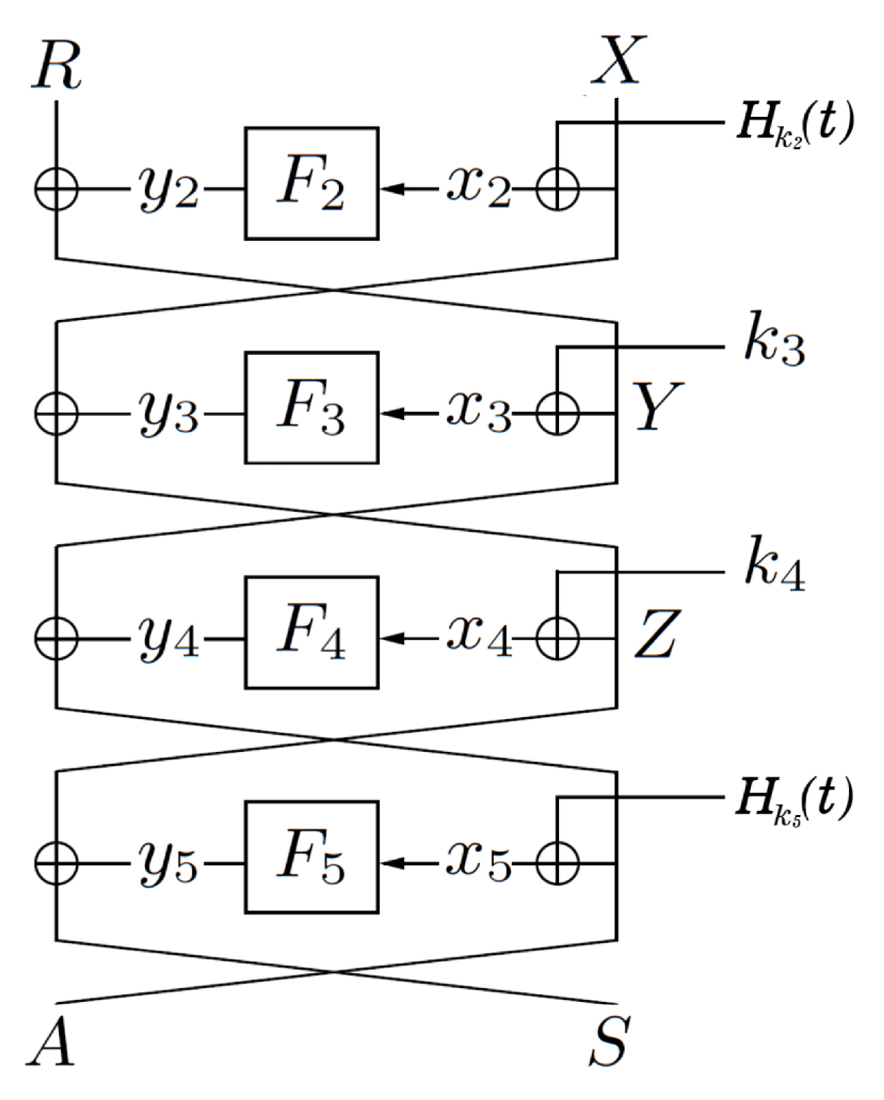
In the following section, we analyze the inner four rounds of $\mathsf{TKAF}$ which depicts in Figure 4. We denote ${\mathcal{Q}}_E^{*}({\mathit{F}}_1,{\mathit{F}}_6)$ the set of tuples in the form $(t,RX,AS)$, which is induced by peeling off outer two rounds. Similar with [24], we also write ${\mathit{F}}^{*}=({\mathit{F}}_2,{\mathit{F}}_3,{\mathit{F}}_4,{\mathit{F}}_5)$, further denote

$$\begin{array}{c}\hfill \mathsf{p}(\tau ,{\mathit{F}}_1,{\mathit{F}}_6)=\mathrm{Pr}\left[{\mathit{F}}^{*}\stackrel{\$}{\leftarrow }{\left(\mathcal{F}\left(n\right)\right)}^4:{\mathsf{TKAF}}_k^{{\mathit{F}}^{*}}⊢{\mathcal{Q}}_E^{*}({\mathit{F}}_1,{\mathit{F}}_6)|{\mathit{F}}_i⊢{\mathcal{Q}}_{F_i},i=1,2,3,4,5,6\right].\end{array}$$

Lemma 4

(From [24]). Assume that there exists a function $\phi :{\left(\mathcal{F}\left(n\right)\right)}^2\times \mathcal{K}\to \left[0,\infty \right)$ such that for any good $({\mathit{F}}_1,{\mathit{F}}_6)$, it holds

$${\displaystyle \mathsf{p}(\tau ,{\mathit{F}}_1,{\mathit{F}}_6)/\prod _{i=0}^{q_e-1}\left(\frac{1}{N^2-i}\right)\ge 1-\phi ({\mathit{F}}_1,{\mathit{F}}_6,k)}.$$

(3)

Then we have

$$\begin{array}{ccc}\hfill \frac{{\mathrm{Pr}}_{re}(\tau ,k)}{{\mathrm{Pr}}_{id}(\tau ,k)}\ge 1& -\hfill & \hfill \mathrm{Pr}\left[\mathsf{Bad}({\mathit{F}}_1,{\mathit{F}}_6)|{\mathit{F}}_1⊢{\mathcal{Q}}_{F_1},{\mathit{F}}_6⊢{\mathcal{Q}}_{F_6}\right]\\ \hfill & -\hfill & \hfill {\mathbb{E}}_{{\mathit{F}}_1,{\mathit{F}}_6}\left[\phi ({\mathit{F}}_1,{\mathit{F}}_6,k)|{\mathit{F}}_1⊢{\mathcal{Q}}_{F_1},{\mathit{F}}_6⊢{\mathcal{Q}}_{F_6}\right].\end{array}$$

Lemma 5.

For any fixed good tuple $({\mathit{F}}_1,{\mathit{F}}_6)$, there exists a function $\phi ({\mathit{F}}_1,{\mathit{F}}_6,k)$ of the function pair and the round- key vector k such that the inequality (3) mentioned in Lemma 4. Then,

$$\begin{array}{cc}\hfill {\mathbb{E}}_{{\mathit{F}}_1,{\mathit{F}}_6,k}\left[\phi ({\mathit{F}}_1,{\mathit{F}}_6,k)\right]& \le 4q_e^2{\epsilon }^2+\frac{7q_e^3+20q_e^2{q}_f+12q_e{q}_f^2}{N^2}\hfill \\ \hfill & +\frac{4q_e^3\epsilon +4q_e^2{q}_f\epsilon +4q_e^2\epsilon +6q_e{q}_f\epsilon }{N}.\hfill \end{array}$$

(4)

Proof. 

Due to the space constraints, the full proof must be deferred to Appendix A. In the following, we only present a proof sketch and the core conclusions. At the beginning of the proof, we define some notations and values in order to present the proof process.

We divide the transcripts in ${\mathcal{Q}}_E^{*}({\mathit{F}}_1,{\mathit{F}}_6)$ into four sets:

• ${\mathcal{G}}_1=\left\{\right|\mathcal{ID}\left(X\right)|=\left|\mathcal{ID}\left(A\right)\right|=1,and{H}_{k_2}\left(t\right)\oplus X\notin Dom{\mathcal{F}}_2\wedge H_{k_5}\left(t\right)\oplus X\notin Dom{\mathcal{F}}_5\}$;
• ${\mathcal{G}}_2=\{H_{k_2}\left(t\right)\oplus X\backslash Dom{\mathcal{F}}_2\}$;
• ${\mathcal{G}}_3=\{H_{k_5}\left(t\right)\oplus A\backslash Dom{\mathcal{F}}_5\}$;
• ${\mathcal{G}}_4=\left\{\right|\mathcal{ID}\left(X\right)|\ge 2or|\mathcal{ID}\left(A\right)|\ge 2\}$.

Then we denote ${\mathsf{E}}_{{\mathcal{G}}_1}$, ${\mathsf{E}}_{{\mathcal{G}}_2}$, ${\mathsf{E}}_{{\mathcal{G}}_3}$ and ${\mathsf{E}}_{{\mathcal{G}}_4}$ by the events that ${\mathsf{TKAF}}_{H_k\left(t\right)}^{{\mathit{F}}^{*}}⊢{\mathcal{G}}_1,{\mathcal{G}}_2,{\mathcal{G}}_3$ and ${\mathcal{G}}_4$ respectively, and let ${\beta }_1=\left|{\mathcal{G}}_2\right|$, ${\beta }_2=\left|{\mathcal{G}}_3\right|$, ${\beta }_3=\left|{\mathcal{G}}_4\right|$. We list ${\mathcal{G}}_i=\{(t,RX,AS),\dots ,(t,R_{|{\mathcal{G}}_i|}{X}_{|{\mathcal{G}}_i|},A_{|{\mathcal{G}}_i|}{S}_{|{\mathcal{G}}_i|})\}$ with some arbitrary orders. Denote ${\mathsf{E}}_{|{\mathcal{G}}_i|}$ the event that ${\mathsf{TKAF}}_{H_k\left(t\right)}^{{\mathit{F}}^{*}}$ extends the i-th tuple $(t,R_i{X}_i,A_i{S}_i)$. We define four sets of “collision position”:

$$\begin{array}{cc}\hfill Ext{\mathcal{F}}_3^{\left(l\right)}& \stackrel{def}{=}\{x_3:\exists (t,R_i{X}_i,A_i{S}_i)\backslash {\mathcal{G}}_1,i\le l,s.t.x_3=k_3\oplus R_i\oplus {\mathit{F}}_2(H_{k_2}\left(t\right)\oplus X_i)\};\hfill \\ \hfill {\mathcal{G}}_2{\mathcal{F}}_3& \stackrel{def}{=}\{x_3:\exists (t,RX,AS)\backslash {\mathcal{G}}_2,s.t.x_3=k_3\oplus R\oplus Img{F}_2(H_{k_2}\left(t\right)\oplus X)\};\hfill \\ \hfill Ext{\mathcal{F}}_4^{\left(l\right)}& \stackrel{def}{=}\{x_4:\exists (t,R_i{X}_i,A_i{S}_i)\backslash {\mathcal{G}}_1,i\le l,s.t.x_4=k_4\oplus S_i\oplus {\mathit{F}}_5(H_{k_5}\left(t\right)\oplus A_i)\};\hfill \\ \hfill {\mathcal{G}}_3{\mathcal{F}}_4& \stackrel{def}{=}\{x_4:\exists (t,RX,AS)\backslash {\mathcal{G}}_3,s.t.x_4=k_4\oplus S\oplus Img{F}_5(H_{k_5}\left(t\right)\oplus A)\}.\hfill \end{array}$$

For convenience, we denote two values $e_3^{\left(l\right)}=|Ext{\mathcal{F}}_3^{\left(l\right)}\setminus Dom{\mathcal{F}}_3|$, and $e_4^{\left(l\right)}=$$|Ext{\mathcal{F}}_4^{\left(l\right)}\setminus Dom{\mathcal{F}}_4|$, which are the quantities of choices in the sets. Finally, the function ${\mathsf{Num}}_3^{\left(l\right)}\left(y_3\right)$ is the number of pre-images $y_3$, which belongs to the set $Dom{\mathcal{F}}_3\cup Ext{\mathcal{F}}_3^{\left(l\right)}$. That is ${\mathsf{Num}}_3^{\left(l\right)}\left(y_3\right)\stackrel{def}{=}\left|\{x_3\backslash Dom{\mathcal{F}}_3\cup Ext{\mathcal{F}}_3^{\left(l\right)}:{\mathit{F}}_3\left(x_3\right)=y_3\}\right|$.

Since we have these definitions mentioned above, we can lower bound

$$\mathsf{p}(\tau ,{\mathit{F}}_1,{\mathit{F}}_6)=\mathrm{Pr}\left[{\mathsf{E}}_{{\mathcal{G}}_1}\wedge {\mathsf{E}}_{{\mathcal{G}}_2}\wedge {\mathsf{E}}_{{\mathcal{G}}_3}\wedge {\mathsf{E}}_{{\mathcal{G}}_4}|\mathit{F}⊢{\mathcal{Q}}_F\right].$$

Analyzing these four sets in turn. First, we consider $\mathrm{Pr}\left[{\mathsf{E}}_{{\mathcal{G}}_1}|\mathit{F}⊢{\mathcal{Q}}_F\right].$ There are three cases for each transcript $(t,RX,AS)\backslash {\mathcal{G}}_1$:

(i)

The two intermediate values Y and Z derived from ${\mathit{F}}_2$ and ${\mathit{F}}_5$ will not collide with the values that have been queried in the past time. So, the probability of this case is at least

$$\left(1-\frac{q_f+e_3^{(l+1)}+\left|{\mathcal{G}}_2{\mathcal{F}}_3\right|}{N}\right)\left(1-\frac{q_f+e_4^{(l+1)}+\left|{\mathcal{G}}_3{\mathcal{F}}_4\right|}{N}\right)\frac{1}{N^2},$$

(ii)

The intermediate value Y collides with some values of the past queries, but Z is still “free”. So, the probability of this case is at least

$$\begin{array}{c}\hfill \left(\frac{q_f+e_3^{\left(l\right)}}{N}-\frac{{\sum }_{x_4\backslash {\mathcal{G}}_3{\mathcal{F}}_4}{\mathsf{Num}}_3^{\left(l\right)}(X_{l+1}\oplus k_4\oplus x_4)}{N}-\frac{q_f^2}{N^2}-\frac{(2q_f+q_e)(q_f+q_e)}{N^2}\right)\frac{1}{N^2}.\end{array}$$

(iii)

This case is symmetrical to the second one, where Z collides with some past values, but Y is “free”. The probability is at least

$$\left(\frac{q_f+e_4^{\left(l\right)}}{N}-\frac{{\sum }_{x_3\backslash {\mathcal{G}}_2{\mathcal{F}}_3}{\mathsf{Num}}_4^{\left(l\right)}(A_{l+1}\oplus k_3\oplus x_3)}{N}-\frac{(2q_f+q_e)(q_f+q_e)}{N^2}\right)\frac{1}{N^2}.$$

Summing over the above five cases, we have

$$\begin{array}{cc}\hfill {\mathbb{E}}_k\left[\mathrm{Pr}\left[{\mathsf{E}}_{{\mathcal{G}}_1}|\mathit{F}⊢{\mathcal{Q}}_F\right]\right]& \ge (1-\frac{q_e{q}_f^2}{N^2}-\frac{2q_e(2q_f+q_e)(q_f+q_e)}{N^2}\hfill \\ \hfill & -\frac{(q_f+2q_e)({\beta }_1+{\beta }_2)}{N})\frac{1}{N^{2|{\mathcal{G}}_1|}}.\hfill \end{array}$$

Then, we analyze ${\mathsf{E}}_{{\mathcal{G}}_2}$, ${\mathsf{E}}_{{\mathcal{G}}_3}$, and ${\mathsf{E}}_{{\mathcal{G}}_4}$. The events ${\mathsf{E}}_{{\mathcal{G}}_2}$ and ${\mathsf{E}}_{{\mathcal{G}}_3}$ can be considered simultaneously. For the rest events, we need to upper- bound the corresponding “bad” events, then consider the efficiency of introducing tweak. Through this method, we can lower bound these three events. See Appendix A for more details about the proof.

For the proof, we have the results of the following three events:

$$\begin{array}{cc}\hfill \mathrm{Pr}\left[{\mathsf{E}}_{{\mathcal{G}}_2}\wedge {\mathsf{E}}_{{\mathcal{G}}_3}|{\mathsf{E}}_{{\mathcal{G}}_1}\wedge \mathit{F}⊢{\mathcal{Q}}_F\right]& \ge (1-\mathrm{Pr}\left[{\mathsf{Bad}}_1\left({\mathit{F}}_3\right)\right]-\mathrm{Pr}\left[{\mathsf{Bad}}_2\left({\mathit{F}}_4\right)\right])\hfill \\ \hfill & ·\mathrm{Pr}\left[{\mathsf{E}}_{{\mathcal{G}}_2}\wedge {\mathsf{E}}_{{\mathcal{G}}_3}|\neg {\mathsf{Bad}}_1\left({\mathit{F}}_3\right)\wedge \neg {\mathsf{Bad}}_2\left({\mathit{F}}_4\right)\right]\hfill \\ \hfill & \ge \left(1-\frac{({\beta }_1+{\beta }_2)(q_f+q_e)}{N}-({\beta }_1+{\beta }_2)\epsilon \right)\hfill \\ \hfill & ·\frac{1}{N^{2\left(\right|{\mathcal{G}}_2|+|{\mathcal{G}}_3\left|\right)}};\hfill \end{array}$$

$$\begin{array}{c}\hfill \mathrm{Pr}\left[{\mathsf{E}}_{{\mathcal{G}}_4}|{\mathsf{E}}_{{\mathcal{G}}_1}\wedge {\mathsf{E}}_{{\mathcal{G}}_2}\wedge {\mathsf{E}}_{{\mathcal{G}}_3}\wedge \mathit{F}⊢{\mathcal{G}}_F\right]\ge \left(1-\mathrm{Pr}\left[{\mathsf{Bad}}_3({\mathit{F}}_2,{\mathit{F}}_5)\right]\right)·\frac{1}{N^{2|{\mathcal{G}}_4|}}\\ \hfill \ge \left(1-\frac{2{\beta }_3(q_f+q_e)}{N}-2{\beta }_3\epsilon \right)·\frac{1}{N^{2|{\mathcal{G}}_4|}}.\end{array}$$

Finally, we sum up all four events, i.e.,

$$\begin{array}{cc}\hfill \mathsf{p}(\tau ,{\mathit{F}}_1,{\mathit{F}}_6)& =\mathrm{Pr}\left[{\mathsf{E}}_{{\mathcal{G}}_1}\wedge {\mathsf{E}}_{{\mathcal{G}}_2}\wedge {\mathsf{E}}_{{\mathcal{G}}_3}\wedge {\mathsf{E}}_{{\mathcal{G}}_4}|\mathit{F}⊢{\mathcal{G}}_F\right]\hfill \\ \hfill & \ge (1-{\theta }_1)(1-{\theta }_2)(1-{\theta }_3)\frac{1}{N^{2\left(\right|{\mathcal{G}}_1|+|{\mathcal{G}}_2|+|{\mathcal{G}}_3|+|{\mathcal{G}}_4\left|\right)}}\hfill \\ \hfill & \ge (1-({\theta }_1+{\theta }_2+{\theta }_3))\frac{1}{N^{2q_e}},\hfill \end{array}$$

where ${\theta }_1$, ${\theta }_2$, ${\theta }_3$ are (A1), (A2) and (A3) respectively, furthermore $|{\mathcal{G}}_1|+|{\mathcal{G}}_2|+|{\mathcal{G}}_3|+|{\mathcal{G}}_4|=q_e$. We note that

$$\begin{array}{c}\hfill \frac{1}{N^{2q_e}}/\prod _{i=0}^{q_e-1}\frac{1}{N^2-i}\ge {(1-\frac{q_e}{N^2})}^{q_e}\ge 1-\frac{q_e^2}{N^2}\ge 1-\frac{q_e^3}{N^2},\end{array}$$

then for (3), we have

$$\begin{array}{cc}\hfill {\mathbb{E}}_k\left[\phi ({\mathit{F}}_1,{\mathit{F}}_6,k)\right]& \le \frac{(3q_e+2q_f)({\beta }_1+{\beta }_2)+2{\beta }_3(q_e+q_f)}{N}\hfill \\ \hfill & +\frac{2q_e(q_e+2q_f)(q_e+q_f)+q_e^3}{N^2}+\frac{q_e{q}_f^2}{N^2}+({\beta }_1+{\beta }_2+2{\beta }_3)\epsilon .\hfill \end{array}$$

We know that ${\beta }_1$, ${\beta }_2$, and ${\beta }_3$ depend on $({\mathit{F}}_1,{\mathit{F}}_6)$. We consider them respectively, focusing on ${\beta }_1$ firstly. For each $(t,RX,AS)\backslash {\mathcal{Q}}_E^{*}({\mathit{F}}_1,{\mathit{F}}_6)$, if $H_{k_1}\left(t\right)\oplus R\backslash Dom{\mathcal{F}}_1$, then it must be $H_{k_2}\left(t\right)\oplus X\notin Dom{\mathcal{F}}_2$ because of ¬(A-2). Thus, on the condition of ${\mathit{F}}_1⊢{\mathcal{Q}}_{F_1}$, ${\mathit{F}}_1(H_{k_1}\left(t\right)\oplus R)$ keeps uniform, then we have

$$\mathrm{Pr}\left[H_{k_2}\left(t\right)\oplus L\oplus {\mathit{F}}_1(H_{k_1}\left(t\right)\oplus R)\backslash Dom{\mathcal{F}}_2\right]\le \frac{q_f}{N}.$$

Therefore, ${\mathbb{E}}_k\left[{\beta }_1\right]\le \frac{q_e{q}_f}{N}.$ The analysis method of ${\beta }_2$ is symmetric with ${\beta }_1$, by the uniformity of ${\mathit{F}}_6$, we have ${\mathbb{E}}_k\left[{\beta }_2\right]\le \frac{q_e{q}_f}{N}.$

To this end, we consider ${\beta }_3$. For the fixed transcript $(t,LR,ST)$ such that $H_{k_1}\left(t\right)\oplus R\notin Dom{\mathcal{F}}_1$, give a distinct $(t^{\prime },L^{\prime }{R}^{\prime },S^{\prime }{T}^{\prime })$. If $t\ne t^{\prime }$ but $LR=L^{\prime }{R}^{\prime }$, for the uniformity of H, we have

$$\mathrm{Pr}\left[X=X^{\prime }\right]=\mathrm{Pr}\left[L\oplus {\mathit{F}}_1(H_{k_1}\left(t\right)\oplus R)=L^{\prime }\oplus {\mathit{F}}_1(H_{k_1}\left(t^{\prime }\right)\oplus R^{\prime })\right]\le \epsilon ;$$

if $t=t^{\prime }$ and $R=R^{\prime }$, then it must be $L\ne L^{\prime }$, thus $X=X^{\prime }$ is impossible; if $t=t^{\prime }$ and $L=L^{\prime }$ but $R\ne R^{\prime }$, on account of $H_{k_1}\left(t\right)\oplus R\notin Dom{\mathcal{F}}_1$, then ${\mathit{F}}_1(H_{k_1}\left(t\right)\oplus R)$ keeps uniformly random conditioned on ${\mathit{F}}_1⊢{\mathcal{Q}}_{F_1}$, therefore $\mathrm{Pr}\left[X=X^{\prime }\right]=\frac{1}{N}$. In addition, the choices of distinct pairs $(t,LR,ST)$ and $(t^{\prime },L^{\prime }{R}^{\prime },S^{\prime }{T}^{\prime })$ are at most $q_e^2$. Thus Thus, we have

$$\begin{array}{c}\hfill {\mathbb{E}}_k\left[\left|\right\{(t,LR,ST):H_{k_1}\left(t\right)\oplus R\notin Dom{\mathcal{F}}_1,and\exists (t^{\prime },L^{\prime }{R}^{\prime },S^{\prime }{T}^{\prime })s.t.X=X^{\prime }\left\}\right|\right]\\ \hfill \le q_e^2\epsilon +q_e^2(1-\epsilon )\frac{1}{N}\le q_e^2\epsilon +\frac{q_e^2}{N}.\end{array}$$

For $H_{k_1}\left(t\right)\oplus R\backslash Dom{\mathcal{F}}_1$, the number of the transcripts $(t,LR,ST)$ which meet the above conditions is $n_{\left(1\right)}\left(k\right)$. We have

$${\mathbb{E}}_k\left[\left|\right\{(t,LR,ST):\exists (t^{\prime },L^{\prime }{R}^{\prime },S^{\prime }{T}^{\prime })s.t.X=X^{\prime }\left\}\right|\right]\le \frac{q_e^2}{N}+q_e^2\epsilon +n_{\left(1\right)}\left(k\right).$$

Symmetrically,

$${\mathbb{E}}_k\left[\left|\right\{(t,LR,ST):\exists (t^{\prime },L^{\prime }{R}^{\prime },S^{\prime }{T}^{\prime })s.t.A=A^{\prime }\left\}\right|\right]\le \frac{q_e^2}{N}+q_e^2\epsilon +n_{\left(6\right)}\left(k\right).$$

Thus, we have

$${\mathbb{E}}_k\left[{\beta }_3\right]\le \frac{2q_e^2}{N}+2q_e^2\epsilon +n_{\left(1\right)}\left(k\right)+n_{\left(6\right)}\left(k\right).$$

Finally, $H_{k_1}\left(t\right)$ and $H_{k_6}\left(t\right)$ are uniform in $2^n$ possible choices,

$${\mathbb{E}}_k\left[n_{\left(1\right)}\left(k\right)\right]={\mathbb{E}}_k\left[n_{\left(6\right)}\left(k\right)\right]=\sum _{(t,LR,ST)\backslash {\mathcal{Q}}_E}\sum _{(x_1,y_1)\backslash {\mathcal{Q}}_{F_1}}\mathrm{Pr}\left[H_{k_1}\left(t\right)=R\oplus x_1\right]\le \frac{q_e{q}_f}{N}.$$

Gathering all the above yields, we have

$$\begin{array}{cc}\hfill {\mathbb{E}}_{{\mathit{F}}_1,{\mathit{F}}_6,k}\left[\phi ({\mathit{F}}_1,{\mathit{F}}_6,k)\right]& \le \frac{6q_e^2{q}_f+4q_e{q}_f^2}{N^2}+\frac{4q_e{(q_e+q_f)}^2}{N^2}\hfill \\ \hfill & +\frac{2q_e(q_e+2q_f)(q_e+q_f)+q_e^3}{N^2}+\frac{q_e{q}_f^2}{N^2}\hfill \\ \hfill & +\frac{4q_e^2(q_e+q_f)\epsilon }{N}+\frac{2q_e{q}_f\epsilon }{N}\hfill \\ \hfill & +\frac{4q_e(q_e+q_f)\epsilon }{N}+4q_e^2{\epsilon }^2\hfill \\ \hfill & =4q_e^2{\epsilon }^2+\frac{7q_e^3+20q_e^2{q}_f+12q_e{q}_f^2}{N^2}\hfill \\ \hfill & +\frac{4q_e^3\epsilon +4q_e^2{q}_f\epsilon +4q_e^2\epsilon +6q_e{q}_f\epsilon }{N},\hfill \end{array}$$

as claimed in (4). □

Now we have Lemma 2, Lemma 4, and (2), we obtain

$$\begin{array}{cc}\hfill \frac{{\mathrm{Pr}}_{re}\left(\tau \right)}{{\mathrm{Pr}}_{id}\left(\tau \right)}\ge 1-(\frac{3q_e{q}_f^2}{N^2}& +{\mathbb{E}}_k\left[\mathrm{Pr}\left[\mathsf{Bad}({\mathit{F}}_1,{\mathit{F}}_6)|{\mathit{F}}_1⊢{\mathcal{Q}}_{F_1},{\mathit{F}}_6⊢{\mathcal{Q}}_{F_6}\right]\right]\hfill \\ \hfill & +{\mathbb{E}}_k\left[{\mathbb{E}}_{{\mathit{F}}_1,{\mathit{F}}_6}\left[\phi ({\mathit{F}}_1,{\mathit{F}}_6,k)|{\mathit{F}}_1⊢{\mathcal{Q}}_{F_1},{\mathit{F}}_6⊢{\mathcal{Q}}_{F_6}\right]\right]).\hfill \end{array}$$

For the expectation ${\mathbb{E}}_k\left[\mathrm{Pr}\left[\mathsf{Bad}({\mathit{F}}_1,{\mathit{F}}_6)|{\mathit{F}}_1⊢{\mathcal{Q}}_{F_1},{\mathit{F}}_6⊢{\mathcal{Q}}_{F_6}\right]\right]$, we note that $k_3$ and $k_4$ are uniformly picked from $2^n$ possibilities, then

$${\mathbb{E}}_k\left[n_{(2,3)}\left(k\right)\right]={\mathbb{E}}_k\left[n_{(4,5)}\left(k\right)\right]\le \frac{q_e{q}_f^2}{N}.$$

It has been shown that ${\mathbb{E}}_k\left[n_{\left(1\right)}\left(k\right)\right]={\mathbb{E}}_k\left[n_{\left(6\right)}\left(k\right)\right]\le \frac{q_e{q}_f}{N}$. Then Lemma 3 yields

$$\begin{array}{c}\hfill {\mathbb{E}}_k\left[\mathrm{Pr}\left[\mathsf{Bad}({\mathit{F}}_1,{\mathit{F}}_6)|{\mathit{F}}_1⊢{\mathcal{Q}}_{F_1},{\mathit{F}}_6⊢{\mathcal{Q}}_{F_6}\right]\right]\\ \hfill \le \frac{4q_e^2{q}_f+5q_e{q}_f^2}{N^2}+\frac{2q_e{q}_f^2\epsilon }{N}+4q_e^2{q}_f{\epsilon }^2.\end{array}$$

From all above, by Lemmas 1 and 2, we have proved the conclusion of Theorem 1.

5. Conclusions and Future Work

This paper presents a result of constructing a tweakable block cipher from the $\mathsf{KAF}$ construction. Our work is based on based on the study by Guo et al. [24], we introduce the tweak into their optimized 6-round scheme $\mathsf{KAF}$ in order to achieve the Beyond Birthday-Bound security. We utilize a universal hash function which is called $\epsilon$-almost XOR-universal hash function, with tweak and round-key vector, we rebuild a new tweakable $\mathsf{KAF}$ scheme $\mathsf{TKAF}$ which meets the security of beyond birthday-bound. Finally Finally, by using the H-coefficient technique [25], we prove the security requirement and obtain a better conclusion with fewer rounds. Our approach is to introduce the tweak into the first and last two rounds of Guo’s 6-round $\mathsf{KAF}$ structure, and utilize the universal hash function as the operation method. Can we introduce the tweak directly into the round function without using the universal hash function, and still meeting the beyond birthday-bound security? Or can we use another linear method to introduce a tweak? We leave these as future work.

References

- Liskov, M.; Rivest, R.L.; Wagner, D. Tweakable block ciphers. In Proceedings of the Annual International Cryptology Conference, Santa Barbara, CA, USA, 18–22 August 2002; Springer: Berlin/Heidelberg, Germany, 2002; pp. 31–46. [Google Scholar]
- Landecker, W.; Shrimpton, T.; Terashima, R.S. Tweakable blockciphers with beyond birthday-bound security. In Proceedings of the Annual Cryptology Conference, Santa Barbara, CA, USA, 19–23 August 2012; Springer: Berlin/Heidelberg, Germany, 2012; pp. 14–30. [Google Scholar]
- Andreeva, E.; Bogdanov, A.; Luykx, A.; Mennink, B.; Tischhauser, E.; Yasuda, K. Parallelizable and authenticated online ciphers. In Proceedings of the International Conference on the Theory and Application of Cryptology and Information Security, Bangalore, India, 1–5 December 2013; Springer: Berlin/Heidelberg, Germany, 2013; pp. 424–443. [Google Scholar]
- Rogaway, P. Efficient instantiations of tweakable blockciphers and refinements to modes OCB and PMAC. In Proceedings of the International Conference on the Theory and Application of Cryptology and Information Security, Jeju Island, Korea, 5–9 December 2004; Springer: Berlin/Heidelberg, Germany, 2004; pp. 16–31. [Google Scholar]
- Rogaway, P.; Bellare, M.; Black, J. OCB: A block-cipher mode of operation for efficient authenticated encryption. ACM Trans. Inf. Syst. Secur. (TISSEC) 2003, 6, 365–403. [Google Scholar] [CrossRef]
- Crowley, P. Mercy: A fast large block cipher for disk sector encryption. In Proceedings of the International Workshop on Fast Software Encryption, New York, NY, USA, 10–12 April 2000; Springer: Berlin/Heidelberg, Germany, 2000; pp. 49–63. [Google Scholar]
- Ferguson, N.; Lucks, S.; Schneier, B.; Whiting, D.; Bellare, M.; Kohno, T.; Callas, J.; Walker, J. The Skein hash function family. NIST (Round 3) 2010, 7, 3, submitted. [Google Scholar]
- Schroeppel, R. Hasty pudding cipher specification. In Proceedings of the First AES Candidate Workshop, Ventura, CA, USA, 20–22 August 1998. [Google Scholar]
- Cogliati, B.; Seurin, Y. Beyond-birthday-bound security for tweakable Even-Mansour ciphers with linear tweak and key mixing. In Proceedings of the International Conference on the Theory and Application of Cryptology and Information Security, Auckland, New Zealand, 29 November–3 December 2015; Springer: Berlin/Heidelberg, Germany, 2015; pp. 134–158. [Google Scholar]
- Mennink, B. XPX: Generalized tweakable even-mansour with improved security guarantees. In Proceedings of the Annual International Cryptology Conference, Santa Barbara, CA, USA, 14–18 August 2016; Springer: Berlin/Heidelberg, Germany, 2016; pp. 64–94. [Google Scholar]
- Naito, Y. Tweakable blockciphers for efficient authenticated encryptions with beyond the birthday-bound security. IACR Trans. Symmetric Cryptol. 2017, 1–26. [Google Scholar] [CrossRef]
- Feistel, H. Cryptography and computer privacy. Sci. Am. 1973, 228, 15–23. [Google Scholar] [CrossRef]
- Even, S.; Mansour, Y. A construction of a cipher from a single pseudorandom permutation. J. Cryptol. 1997, 10, 151–161. [Google Scholar] [CrossRef]
- Jean, J.; Nikolić, I.; Peyrin, T. Tweaks and keys for block ciphers: The TWEAKEY framework. In Proceedings of the International Conference on the Theory and Application of Cryptology and Information Security, Kaoshiung, Taiwan, 7–11 December 2014; Springer: Berlin/Heidelberg, Germany, 2014; pp. 274–288. [Google Scholar]
- Cogliati, B.; Lampe, R.; Seurin, Y. Tweaking even-mansour ciphers. In Proceedings of the Annual Cryptology Conference, Santa Barbara, CA, USA, 16–20 August 2015; Springer: Berlin/Heidelberg, Germany, 2015; pp. 189–208. [Google Scholar]
- Cogliati, B.; Seurin, Y. On the provable security of the iterated Even-Mansour cipher against related-key and chosen-key attacks. In Proceedings of the Annual International Conference on the Theory and Applications of Cryptographic Techniques, Sofia, Bulgaria, 26–30 April 2015; Springer: Berlin/Heidelberg, Germany, 2015; pp. 584–613. [Google Scholar]
- Farshim, P.; Procter, G. The related-key security of iterated Even—Mansour ciphers. In Proceedings of the International Workshop on Fast Software Encryption, Istanbul, Turkey, 8–11 March 2015; Springer: Berlin/Heidelberg, Germany, 2015; pp. 342–363. [Google Scholar]
- Granger, R.; Jovanovic, P.; Mennink, B.; Neves, S. Improved masking for tweakable blockciphers with applications to authenticated encryption. In Proceedings of the Annual International Conference on the Theory and Applications of Cryptographic Techniques, Vienna, Austria, 8–12 May 2016; Springer: Berlin/Heidelberg, Germany, 2016; pp. 263–293. [Google Scholar]
- Luby, M.; Rackoff, C. How to construct pseudorandom permutations from pseudorandom functions. SIAM J. Comput. 1988, 17, 373–386. [Google Scholar] [CrossRef]
- Mitsuda, A.; Iwata, T. Tweakable pseudorandom permutation from generalized feistel structure. In Proceedings of the International Conference on Provable Security, Shanghai, China, 30 October–1 November 2008; Springer: Berlin/Heidelberg, Germany, 2008; pp. 22–37. [Google Scholar]
- Lampe, R.; Seurin, Y. Security analysis of key-alternating Feistel ciphers. In Proceedings of the International Workshop on Fast Software Encryption, London, UK, 3–5 March 2014; Springer: Berlin/Heidelberg, Germany, 2014; pp. 243–264. [Google Scholar]
- Goldenberg, D.; Hohenberger, S.; Liskov, M.; Schwartz, E.C.; Seyalioglu, H. On tweaking luby-rackoff blockciphers. In Proceedings of the International Conference on the Theory and Application of Cryptology and Information Security, Kuching, Malaysia, 2–6 December 2007; Springer: Berlin/Heidelberg, Germany, 2007; pp. 342–356. [Google Scholar]
- Yan, H.; Wang, L.; Shen, Y.; Lai, X. Tweaking Key-Alternating Feistel Block Ciphers. In Proceedings of the International Conference on Applied Cryptography and Network Security, Rome, Italy, 9–22 October 2020; Springer: Cham, Switzerland, 2020; pp. 69–88. [Google Scholar]
- Guo, C.; Wang, L. Revisiting key-alternating Feistel ciphers for shorter keys and multi-user security. In Proceedings of the International Conference on the Theory and Application of Cryptology and Information Security, Brisbane, QLD, Australia, 2–6 December 2018; Springer: Cham, Switzerland, 2018; pp. 213–243. [Google Scholar]
- Patarin, J. The “coefficients H” technique. In Proceedings of the International Workshop on Selected Areas in Cryptography, Sackville, NB, Canada, 14–15 August 2008; Springer: Berlin/Heidelberg, Germany, 2008; pp. 328–345. [Google Scholar]
- Chen, S.; Steinberger, J. Tight security bounds for key-alternating ciphers. In Proceedings of the Annual International Conference on the Theory and Applications of Cryptographic Techniques, Copenhagen, Denmark, 11–15 May 2014; Springer: Berlin/Heidelberg, Germany, 2014; pp. 327–350. [Google Scholar]
- Hoang, V.T.; Tessaro, S. Key-alternating ciphers and key-length extension: Exact bounds and multi-user security. In Proceedings of the Annual International Cryptology Conference, Santa Barbara, CA, USA, 14–18 August 2016; Springer: Berlin/Heidelberg, Germany, 2016; pp. 3–32. [Google Scholar]
Figure 1.
10-round tweakable Key-Alternating Feistel cipher presented by Yan et al.
Figure 2.
A distinguisher distinguish the real world and the ideal world.
Figure 3.
A tweakable Key-Alternating Feistel cipher with 6 rounds.
Figure 4.
Inner 4 rounds of the tweakable Key-Alternating Feistel cipher.
Publisher’s Note: MDPI stays neutral with regard to jurisdictional claims in published maps and institutional affiliations. |
© 2021 by the authors. Licensee MDPI, Basel, Switzerland. This article is an open access article distributed under the terms and conditions of the Creative Commons Attribution (CC BY) license (https://creativecommons.org/licenses/by/4.0/).
Share and Cite
MDPI and ACS Style
Jiang, M.; Wang, L. Almost-Minimal-Round BBB-Secure Tweakable Key-Alternating Feistel Block Cipher. Symmetry 2021, 13, 649. https://doi.org/10.3390/sym13040649
AMA Style
Jiang M, Wang L. Almost-Minimal-Round BBB-Secure Tweakable Key-Alternating Feistel Block Cipher. Symmetry. 2021; 13(4):649. https://doi.org/10.3390/sym13040649
Chicago/Turabian StyleJiang, Ming, and Lei Wang. 2021. "Almost-Minimal-Round BBB-Secure Tweakable Key-Alternating Feistel Block Cipher" Symmetry 13, no. 4: 649. https://doi.org/10.3390/sym13040649
Note that from the first issue of 2016, this journal uses article numbers instead of page numbers. See further details here.