Multi-Modal Evolutionary Deep Learning Model for Ovarian Cancer Diagnosis

Abstract

Ovarian cancer (OC) is a common reason for mortality among women. Deep learning has recently proven better performance in predicting OC stages and subtypes. However, most of the state-of-the-art deep learning models employ single modality data, which may afford low-level performance due to insufficient representation of important OC characteristics. Furthermore, these deep learning models still lack to the optimization of the model construction, which requires high computational cost to train and deploy them. In this work, a hybrid evolutionary deep learning model, using multi-modal data, is proposed. The established multi-modal fusion framework amalgamates gene modality alongside with histopathological image modality. Based on the different states and forms of each modality, we set up deep feature extraction network, respectively. This includes a predictive antlion-optimized long-short-term-memory model to process gene longitudinal data. Another predictive antlion-optimized convolutional neural network model is included to process histopathology images. The topology of each customized feature network is automatically set by the antlion optimization algorithm to make it realize better performance. After that the output from the two improved networks is fused based upon weighted linear aggregation. The deep fused features are finally used to predict OC stage. A number of assessment indicators was used to compare the proposed model to other nine multi-modal fusion models constructed using distinct evolutionary algorithms. This was conducted using a benchmark for OC and two benchmarks for breast and lung cancers. The results reveal that the proposed model is more precise and accurate in diagnosing OC and the other cancers.

1. Introduction

Ovarian cancer (OC) is indicated as the fifth prevalent reason for cancer-related deaths between women. Most cases (75%) happen in post-menopausal patients, with incidence of 40 for each 100,000 per year, in patients aged over 50. Early detection of such disease significantly raises 5-year survival, from 3% (in Stage IV) to 90% (in Stage I) [1]. Histopathology evaluation represents the gold standard by which OC is diagnosed and identified into histological types. Cellular morphology interpretation defines the various OC types and guides the treatment planning [2], which is best performed through expert pathologists in ovarian tumors. However, inter-observer variations in grading have been reported. These variations in histopathologic interpretation will cause not only inaccurate prognostic prediction and suboptimal treatments but also loss of life quality [3].

This sheds light on the urgent need to construct computational methods that can precisely predict OC. Towards this goal, a number of OC diagnosis models [4,5,6] were developed during the past decade, based upon the single modal histopathological images, because it can reflect morphological characteristics of the cells that are closely connected to the OC aggressiveness. Besides histopathological images, it has also been known that the gene expression levels and genetic mutations can implicitly influence the development of cancers by accelerating the cell division rates and modifying the micro-environment of tumor [7]. Therefore, the genomic features represent important indicators for driving diagnosis practices, which contain a catalog of gene expression signatures, sequence mutations, focal variations in DNA copy numbers, and methylation alterations [8].

Given the heterogeneity and complexity of cancer survival prediction, the newly developed whole-slide histopathology scanners, as well as high-throughput omics profiling [6] coupled with innovative machine learning (ML) algorithms, the recent studies [9,10,11,12] have shown that the integrative analyses of both patient’s genomic data and pathology images are of high efficiency in cancers assessment. Sun et al. [9] have integrated the pathology images and genomic data for predicting breast cancer outcome. A multiple kernel learning approach was employed to join the heterogeneous information of the two modalities. The approach achieved 0.8022 as accuracy and 0.7273 of precision. In [10], a multi-modal multi-task feature selection approach was introduced for diagnosing cancers, namely, M2DP. In which, features from both gene expression data and pathology images were extracted, then the M2DP model was implemented for identifying diagnosis related features. For each patient, the selected features were utilized for the diagnosis by using AdaBoosting. The model was tested using a benchmark for breast cancer and another one for lung cancer, showing accuracy of 72.53 and 70.08%, respectively. Zhang et al. [11] introduced a multiple kernel approach for predicting lung carcinomas by amalgamating genomic data with pathological features of images, which showed 0.8022 as accuracy. Liu et al. [12] proposed a multi-modal deep learning model for predicting breast cancer subordinate type. The model fully extracted the deep-seated features from gene and image modalities by using a deep learning model, and finally fused the different features using weighted linear aggregation. The prediction accuracy was 88.07%.

Recent advances in the convolutional neural networks (CNN) and other resembling deep learning models have remarkable implications in medical diagnosis. Kott et al. [13] utilized a deep residual CNN for histopathologic diagnosis of a prostate cancer. The model showed 91.5% accuracy at a coarse-level classification of the image patches into benign and malignant. Ismael et al. [14] proposed a method for automatically classifying brain tumors by using residual networks (ResNet50 architecture). The model accuracy was 0.97 on patient-level. Harangi et al. [15] employed the deep GoogleNet Inception for classifying dermoscopy images. The accuracy reached 0.677. Celik et al. [16] used a deep approach to detect invasive ductal carcinoma from histopathology images. The DenseNet-161 and ResNet-50 were employed. The DenseNet-161 model realized F-score of 92.38% with accuracy of 91.57%. However, in the medical applications field, lots of tasks are based upon long-range dependencies [17]. Recurrent Neural Network (RNN) models are leading methods to deeply learn the longitudinal data. A variant of RNN is long-short-term-memory (LSTM) [18] that captures both long-term and short-term dependencies within sequential data. Gao et al. [19] employed distanced LSTM with time-distanced gates for diagnosing lung cancer by using both real computed tomography images and simulated data. The method realized 0.8905 as F-score. Guo et al. [17] presented a disease inference approach based on symptom sequence extraction from discharge summary using a bidirectional LSTM that achieved F-score of 0.572.

Although deep learning networks have shown promising diagnostic performance, designing an appropriate deep learning model not only demands extremely specialized knowledge but also is a labor- and time-consuming task to a large extent. The recent studies showed also that the expressive power for deep neural network is essential and affects the deep learning. Lu et al. [20] studied how width influences the neural networks expressiveness by showing universal approximation theorem concerning width-bounded ReLU network. In [21], the authors revealed the power of deeper networks in comparison to shallower ones, through proving that the total neurons number needed for approximating natural classes of the multivariate polynomials with m variables increases only linearly with m in case of deep neural network, but increases exponentially when just a single hidden-layer is allowed. Du et al. [22] provided theoretical insight on the generalization ability and optimization landscape of over-parameterized neural network. Qi et al. [23] showed that, in the vector-to-vector regression utilizing the deep neural networks, the generalized loss of mean-absolute-error (MAE) between predicted and expected vectors of features is upper bounded by sum of the approximation error, estimation error, and optimization error.

Therefore, an urgent issue in the deep learning domain is optimization of the model construction. According to recent studies [24,25], the model construction often affects its overall performance and requires to be automatically set. These studies revealed that optimizing the hyperparameters remains a major obstacle in designing the deep learning models, including CNNs. In [24], a genetic algorithm based approach for constructing CNN structure was proposed for automatic analysis of medical images. Gao et al. [25] presented a method for optimizing the CNN structure that integrates binary coding system with gradient-priority particle swarm optimization (PSO) to select the structure. Therefore, it is useful to employ the swarm intelligence optimization techniques for enabling the networks to automatically tune their hyperparameters besides the layer connections and make the optimal utilization of the redundant computing resources. Grey wolf optimizer (GWO) [26], antlion optimization (ALO) [27], crow search (CS) algorithm [28], artificial bee colony (ABC) [29], differential evolution (DE) algorithm [30], whale optimization (WO) algorithm [31], Salp swarm algorithm [32], PSO [33], bat optimization (BAT) algorithm [34], and genetic algorithm (GA) [35] are some biologically-inspired algorithms investigated in optimization purposes.

The goal of this work is to propose a hybrid deep learning model based on the multi-modal data to precisely predict the OC stage. The method combined the data of gene expressions, copy number variants, and the pathological image features, besides considering the heterogeneity of every sole modal data, achieving precise prediction of the OC stages. The main contributions of this paper are summarized as:

• Unlike the state-of-the-art deep learning models which employ single modality data for OC diagnosis and also still lack to the experience of automatic topology construction, a new multi-modal deep learning model is proposed to predict the OC stage. In which, a customized feature extraction network was established to fit each modality’s data and fully extract the deep-seated features, respectively. Each feature network is hybridized with the ALO optimizer to automatically set its topology, which shows stability in processing the longitudinal genomic data and provides optimum image feature maps that realize better performance. The output from the two improved feature networks is finally fused based upon weighted linear aggregation in order to predict the OC stage.
• In total, nine multi-modal fusion models were constructed (with) and without the other different optimization algorithms, and then compared to the proposed model for testing its efficiency in predicting OC stage.
• The established multi-modal deep learning model is applicable to predict other cancers subtypes by integrating features from the gene modal with the pathology image modal.

The rest of this paper is organized as follows; Section 2 is specified for the preliminaries. Section 3 describes the materials and methods. Section 4 details the proposed method. The experiments and results are discussed in Section 4. The conclusions and future works are listed in the last section.

2. Preliminaries

2.1. Convolutional Neural Network Models

Deep learning methods are classified into CNNs, pre-trained unsupervised networks, and basic recurrent neural networks (RNN). CNNs [29,36] encompass a sequence of processing layers with different types. Regular CNNs have convolutional, fully-connected (FC), as well as pooling layers (Figure 1a). The most intensive part in CNNs is the convolutional layers that convolve the 2-D kernels to input feature maps for generating output feature maps. Then, the pooling layers come after the convolutional layers which down-sample output feature map by summarizing its features into patches. The pooling is computed taking the mean of each patch in the feature map, or considering the greatest value in each patch. Eventually, the final FC accomplishes the classification task similar to the conventional artificial neural network (ANN).

2.2. Long-Short-Term-Memory Models

The LSTM is an extension of the basic RNN. This network adds time-dependent features relying on a preceding timestamp and operates as memory cell for remembering data from the preceding timestamp [18,29]. The memory cell $\mathrm{c}$ is controlled through a group of gate networks (Figure 1b), including $f$ forget gate network, $i$ input gate network, and $o$ output gate network. The forget gate decides which information to forget. In other words, it decides which information be eliminated from its past cell states. The input gates $i_t$decide which information would be added to memory cells $c_t$. This behavior determines how much information would be updated and which information would be updated. Output gates $o_t$ decide which information would be used as output.

2.3. Ant Lion Optimizer

ALO is a new biologically-inspired algorithm introduced [27,37] in emulating the natural hunting mechanism of antlions:

Operators of Algorithm. It supposes a population ($Pop$) of ants and antlions in a dimensional ($d$) problem space: $A=\left\{Antlio{n}_i,An{t}_i|i\in Pop\right\}$. A random variable is set using Equation (1), where $Rnd$ is generated in $\left[0, 1\right]$ interval randomly. Ants’ random walks are calculated by normalizing cumulative sum of all iterations using Equation (2), $cs$ computes cumulative sum, $T$ denotes maximum iteration, and $t$ is current iteration. During optimization process, ants’ locations are kept in matrix $L_{ant}$. The ant’s location is the parameter for every solution. The objective function is assessed during optimization and matrix $L_{oa}$ stores the fitness computed for each ant. Likewise, the antlions are hiding within search space, where $L_{antlion}$ and $L_{oa}$ are used to store their positions.

$$\mathrm{S}=\{\begin{array}{c}1, \mathrm{if} (Rnd>0.5)\hfill \\ 0, \mathrm{else}\hfill \end{array}$$

(1)

$$X^t=\left[0,cs\left(2s\left(t_1\right)-1\right),cs\left(2s\left(t_2\right)-1\right),\dots ,cs\left(2s\left(t_T\right)-1\right)\right]$$

(2)

$$L_{ant}=\left[\begin{array}{ccc}an{t}_{\left(1,1\right)}& \dots & an{t}_{\left(1,d\right)}\\ ⋮& ⋮& ⋮\\ an{t}_{\left(k,1\right)}& \dots & an{t}_{\left(k,d\right)}\end{array}\right], L_{oa}=\left[\begin{array}{c}Fi{t}_t\left(\left[an{t}_{\left(1,1\right),}an{t}_{\left(1,2\right),}\dots ,an{t}_{\left(1,d\right)}\right]\right)\\ ⋮\\ Fi{t}_t(\left[an{t}_{\left(k,1\right),}an{t}_{\left(k,2\right),}\dots ,an{t}_{\left(k,d\right)}\right]\end{array}\right]$$

(3)

$${\mathrm{L}}_{\mathrm{antlion}}=\left[\begin{array}{ccc}{\mathrm{antlion}}_{\left(1,1\right)}& \dots & {\mathrm{antlion}}_{\left(1,\mathrm{d}\right)}\\ ⋮& ⋮& ⋮\\ {\mathrm{antlion}}_{\left(\mathrm{k},1\right)}& \dots & {\mathrm{antlion}}_{\left(\mathrm{k},\mathrm{d}\right)}\end{array}\right],{\mathrm{L}}_{\mathrm{oa}}=\left[\begin{array}{c}{\mathrm{Fit}}_{\mathrm{t}}\left(\left[{\mathrm{antlion}}_{\left(1,1\right),}{\mathrm{antlion}}_{\left(1,2\right),}\dots ,{\mathrm{antlion}}_{\left(1,\mathrm{d}\right)}\right]\right)\\ ⋮\\ {\mathrm{Fit}}_{\mathrm{t}}(\left[{\mathrm{antlion}}_{\left(\mathrm{k},1\right),}{\mathrm{antlion}}_{\left(\mathrm{k},2\right),}\dots ,{\mathrm{antlion}}_{\left(\mathrm{k},\mathrm{d}\right)}\right]\end{array}\right]$$

(4)

Random Walks for Ants. Ants change their own positions according to Equation (2). For keeping random walks within the search space, Equation (5) is used to normalize them, $a_i$ and $b_i$denote lower bounds, and upper bounds for the random walk in $ith$ dimension, respectively, while $c_i^t$ and $d_i^t$ refer lower bounds, and upper bounds for the $ith$ dimension at $tth$ iteration.

$$X_i^t=\frac{\left(X_i^t-a_i\right)\times \left(d_i^t-c_i^t\right)}{\left(b_i-a_i\right)}+c_i^t$$

(5)

Trapping in Antlion’s Pits. Ants’ random walks are influenced by antlions’ traps. Equation (6) randomly gives the ants’ walks in hyper sphere identified by the $c$ and $d$ vectors, surrounding a selected antlion. The $Antlio{n}_m^t$ denotes position of selected $mth$ antlion surrounding which ants are trapped.

$$c_i^t=Antlio{n}_m^t+c^t and d_i^t=Antlio{n}_m^t+d^t$$

(6)

Building Trap. Antlion’s hunting ability is modeled using roulette wheel (RW). The ALO algorithm utilizes the RW operator for electing antlions based upon their fitness through the iterations. This mechanism demonstrates high opportunities for catching ants.

Sliding Ants Towards Antlion. Using the foregoing mechanisms, antlions build traps relevant to their fitness and ants have to move randomly. Despite that, antlions shoot sand outwards the pit’s center as soon as they sense any ant inside the trap. This helps slide down any trapped ant tries to escape. For modeling this behavior, the algorithm adaptively reduces hyper sphere radius for ant’s random walk, where $c_i$ and $d_i$ represent the lower bounds, and upper bounds for $ith$ dimension of the considered problem, $I$ refers the ratio, and $L$ denotes the constant parameter controls the exploitation level.

$$c_i^t=\frac{c_i}{I}, d_i^t=\frac{d_i}{I}, and I=L\frac{t}{T}$$

(7)

Catching Prey and Rebuilding the Pit. At this stage, an objective function is assessed. If the ant demonstrated better objective function compared to the selected antlion, it swaps its position with the hunted ant’s latest position to improve its opportunity for catching new one, as follows:

$$Antlio{n}_m^{t+1}=An{t}_h^t if fitness\left(Antlio{n}_m^t\right)<fitness\left(An{t}_h^t\right)$$

(8)

Elitism. The best antlion obtained so far is kept as the elite. It must influence the motions for all ants during the iterations. Consequently, it is supposed that each ant randomly walks surrounding a selected antlion using the RW and elite simultaneously as follows, where $Antlio{n}_{RW}$is the antlion chosen by RW at $tth$ iteration, and $Antlio{n}_{ET}$ denotes the best antlion.

$$An{t}_h^t=\frac{Antlio{n}_{RW}^t+Antlio{n}_{ET}^t}{2}$$

(9)

3. Materials and Methods

This section presents a sufficient description on the methods utilized in this work.

3.1. Dataset

We used a public dataset for prediction of OC stage taken from Cancer Genome Atlas portal, namely, the TCGA-OV: https://portal.gdc.cancer.gov/ (accessed on 2 March 2021). The dataset includes the gene expressions data and copy number variants data of 587 OC patients. In addition, each patient has many pathological images. The gene expressions data and copy variants data are of one dimension, corresponding to one modality type, the pathology images are colored, correspond to another modality type. In this work, we call them gene modal and pathology image modal, respectively. The characteristics of the TCGA-OV multi-modal dataset are detailed in

Table 1. Description of TCGA-OV multimodal dataset.

Clinical Characteristics	Number of Samples
Patients with Serous Ovarian Carcinoma having Clinical Data	N = 587
Stage I	17 (2.90%)
Stage II	30 (5.11%)
Stage III	446 (75.98%)
Stage IV	89 (15.16 %)
Stage Not Available	5 (0.85 %)
Data Category	Number of Attributes
Gene expressions	6426
Copy number variants	24,776
Pathology images for each sample	1–10 images
Total pathology images for all samples.	1375 images

. The number of patients (samples) representing the OC stage is shown. The gene expressions data comprised about 6426 data indicators, while the copy number variants included about 24,776 data indicators. There were also from one to 10 pathological images available for each patient.

3.2. System Architecture

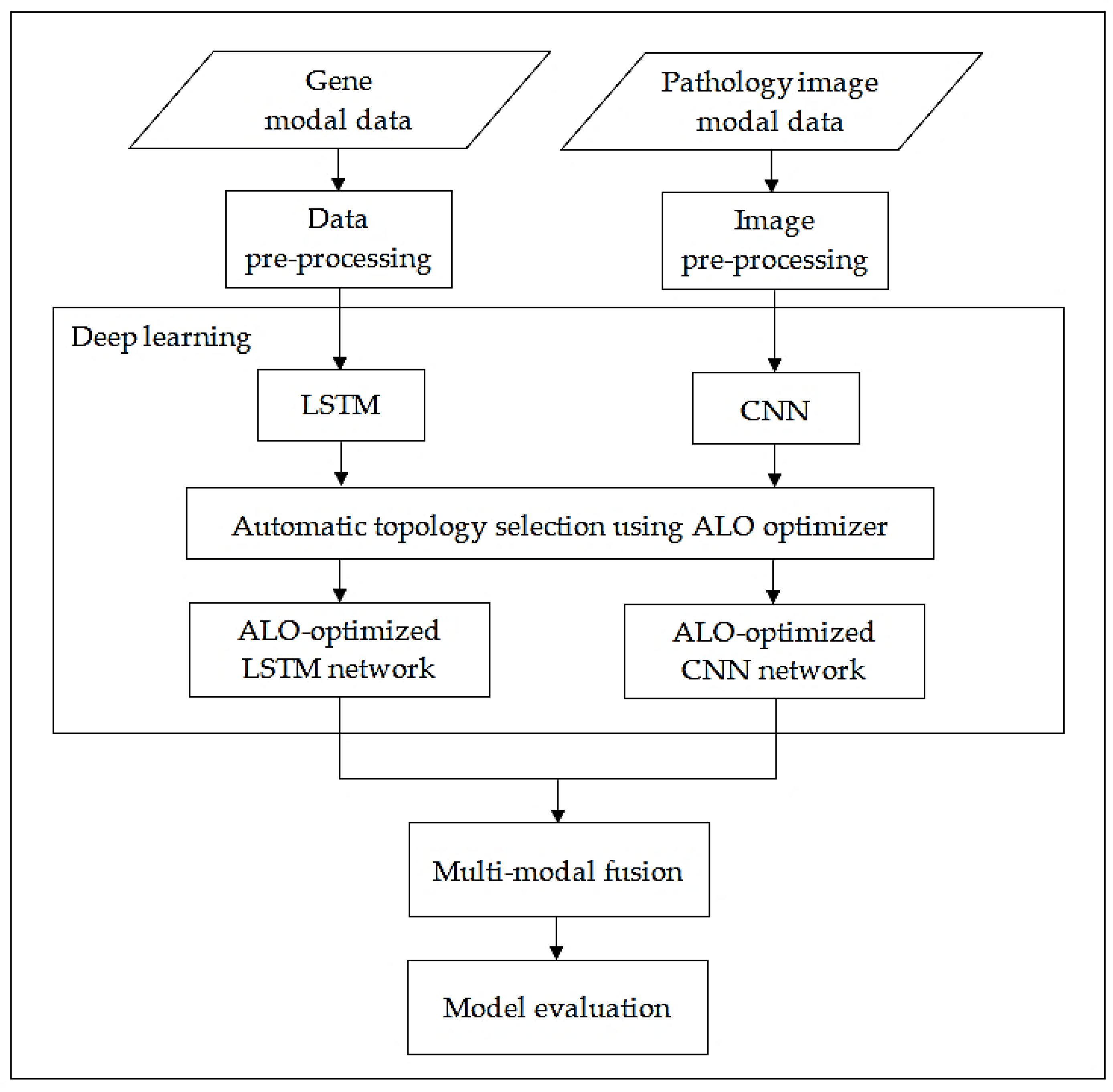
In this work, a hybrid bio-inspired deep learning model using multi-modal data is proposed. We construct a multi-modal fusion framework by integrating gene modality data with histopathology image modality data of OC patients as demonstrated in Figure 2. Based on the different states and forms of each modality, a feature extraction network was established, respectively. In this context, a predictive antlion-optimized LSTM network model is designed to process gene longitudinal data and another predictive antlion-optimized CNN model is designed to efficiently extract abstract features from the pathological images. The topology of both the two networks is automatically selected by the ALO algorithm. The output from the two improved feature extraction networks is then fused based upon weighted linear aggregation. Finally, the deep fused features are finally used to predict the OC stage.

3.3. A Proposed ALO-LSTM Prediction Model Based upon Gene Modality

3.3.1. Data Pre-Processing

The gene modality includes gene expressions data and copy number variants. So as to input the properties of these two data kinds in the network simultaneously, we integrated the data belonging to the same modality, thus the newly consolidated data included 31,202 data indicators. To eliminate the different chemotaxis and dimensional disunity problems after the integration of the two data types, we adopted Z-Score [12] to pre-process the data. The Z-Score is a data standardization method based on computing the average and standard deviation for the original data. The following equation expresses the formula specified for this method:

$$y^{*}=\frac{y+\overline{y}}{\delta }$$

(10)

In the above formula, $y$ denotes the data item value, $\overline{y}$ denotes the data item mean value, and $\delta$ denotes the data item standard deviation value. Due to the Z-Score linear nature, data change is not cause of “failure”, but it improves data performance [12]. The principle component analysis is then applied for reduction in data noise and eliminating redundant. Therefore, the number of items in gene modality data was reduced from 31,202 to 405.

3.3.2. A Structure Design of Improved LSTM

The data of gene modality are big and represented as one-dimensional vectors. The LSTM has proven promise for extracting features from longitudinal data. However, the model accuracy is affected by many architectural factors [38] including the input length ($g$), units number of hidden layer ($u$), number of epochs ($m$), batch size ($b$), initial learning rate ($i$), etc. For instance, if the value of $m$ is too small, it will be difficult for training data to converge; if it is too large, overfitting will occur. Likewise, if the value of $b$ is too small, it will be difficult for training data to converge which will cause underfitting, but if it is too large, required memory will significantly rise. Furthermore, the value of $u$ effects the influence of fitting. Supposing that $m$ ranges in $\left[1–1000\right]$, $u$ ranges in $\left[1–50\right]$, and $b$ ranges in$\left[1–500\right]$. A total of 250,000,000 combinations will result. This will cause a heavy calculation issue, and a reliable algorithm has to be utilized for automatically setting the hyperparameters to balance computational efficiency and predictive performance. The ALO algorithm proved competitive performance in: avoiding local optima, exploitation, improved exploration, and convergence [39]. It is super in many unimodal and multi-modal test functions [40]. The reason behind its quick exploitation and convergence is the adaptive boundary shrinking technique and elitism. The higher exploration results from the employed random walks and RW selection mechanisms which cause population diversity.

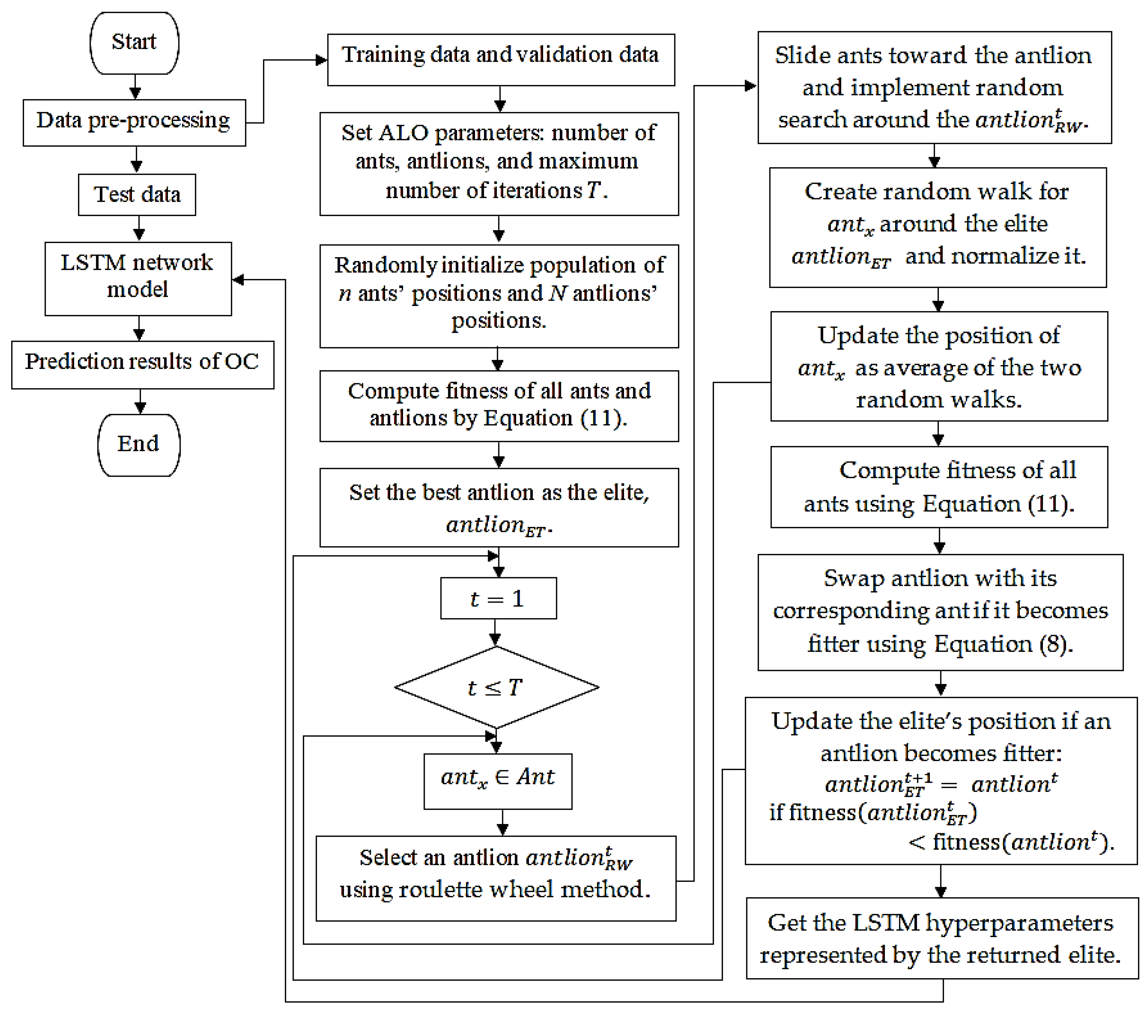
This paper proposed an improved LSTM using ALO algorithm that can well process longitudinal gene data by selecting the suitable input length of the gene modality and discarding unusual input data which can diminish prediction errors. This ALO-optimized LSTM network is not restricted with specific number of LSTM units to sequentially process the gene modal data. Figure 3 shows a flowchart of the model. The optimization procedure is as follows.

Step 1: Data pre-processing. The gene dataset is subdivided into: training, validation, and testing sets.

Step 2: Initialization. The algorithm initially sets population of $n$ ants’ and $N$ antlions’ positions deeming the boundary values for LSTM hyperparameters. Equation (2) is used to obtain initial population.

Step 3: The fitness of all ants and antlions is computed using Equation (11), and the elite $antlio{n}_{ET}$ is defined. The best combination between the LSTM hyperparameters $\alpha$ and CNN hyperparameters $\beta$ on the validation set was found. We used the cross entropy between the feature fusion result $predictio{n}_{fusion}$ and Label as fitness function. Thus the best solution of ($\alpha , \beta$) was that closer to the minimum ($\alpha , \beta$) as follows.

$$\begin{gathered} Min\left(Loss\left(predictio{n}_{fusion}, Label\right)\right) \\ \{\begin{array}{c}\alpha +\beta =1\\ 0\le \alpha \le 1, 0\le \beta \le 1\end{array} \end{gathered}$$

(11)

Step 4: The roulette wheel (RW) method is used to choose an antlion $antlio{n}_{RW}^t$.

Step 5: A random walk for $an{t}_x\in Ant$ is created and normalized by using Equation (5). The position of $an{t}_x$is then updated as the average of the two random walks.

Step 6: The fitness values for all the ants are then computed by Equation (11) and the antlion is swapped with its related ant if it becomes fitter. The elite’s position is updated, if the $antlio{n}_x^t$ has greater fitness than the elite.

Step 7: The previous steps are repeated until reaching maximum iteration $T$.

Step 8: The best individual from ALO is assigned as optimum hyperparameter for the LSTM.

Step 9: The sequential processing of gene data is implemented using Equation (12), where $f_t$ is the forget gate’s activation vector, $i_t$refers the input gate, $o_t$ indicates the output gates, $\sigma \left(x\right)$ denotes sigmoid function, $tanh\left(x\right)$ indicates hyperbolic tangent function, $g_t$ is an input modulation, h_t is a hidden LSTM state, $x\otimes y$ denotes the element-wise multiplication operation between $x$ and $y$, $t$ denotes the current timestamp, $W$ and $B$ are the weights and bias for each gate.

$$\begin{gathered} f_t=\sigma \left(W_{fx}^T{x}_t+W_{fc}^T{c}_{t-1}+B_f\right) \\ {i}_t=\sigma \left(W_{ix}^T{x}_t+W_{ic}^T{c}_{t-1}+B_i\right) \\ {g}_t=\tanh \left(W_{gx}^T{x}_t+W_{gc}^T{c}_{t-1}+B_g\right) \\ {c}_t=f_t\otimes c_{t-1}+i_t\otimes g_t \\ {o}_t=\sigma \left(W_{ox}^T{x}_t+W_{oc}^T{c}_{t-1}+B_o\right) \\ {h}_t=o_t\tan \mathrm{h}\otimes \left(c_t\right) \\ \sigma \left(x\right)={\left(1+e^{-x}\right)}^{-1} \\ tanh\left(x\right)=\frac{e^x-e^{-x}}{e^x+e^{-x}}=\frac{1-e^{-2x}}{1+e^{-2x}}=2\sigma \left(2x\right)-1 \end{gathered}$$

(12)

Step 10: The validation and training sets are used to train the Improved LSTM.

Step 11: LSTM is fitted by the testing inputs of gene data to predict testing outputs.

The optimal hyperparameters selected by the ALO to tune the LSTM topology are demonstrated in

Table 2. Topology of the LSTM selected by ALO.

LSTM Parameters	Range/Value	Best Selected Values (Elite’s Ones)
Input length	$\left[1–405\right]$	90
Units number of hidden layer	$\left[1–50\right]$	37
Number of epochs	$\left[10–50\right]$	14
Batch size	$\left[32–128\right]$	64
L2-regularization factor	$\left[0.00001–0.01\right]$	0.005
Initial learning rate	$\left[0.1–0.5\right]$	0.3
Learn rate drop factor	$\left[0.01–0.9\right]$	0.8
Learn rate drop period	$\left[10–100\right]$	42
Gradient threshold	$\left[1–10\right]$	4

. The range of input length was assigned within $\left[1–405\right]$. The Units number of hidden layer was assigned within $\left[1–50\right]$ and the batch size was assigned within the range [1–500]. Additionally, the best input length of gene modality data was reduced to 90 individuals.

3.4. A Proposed ALO-CNN Prediction Model Based upon Pathology Image Modality

3.4.1. Image Pre-Processing

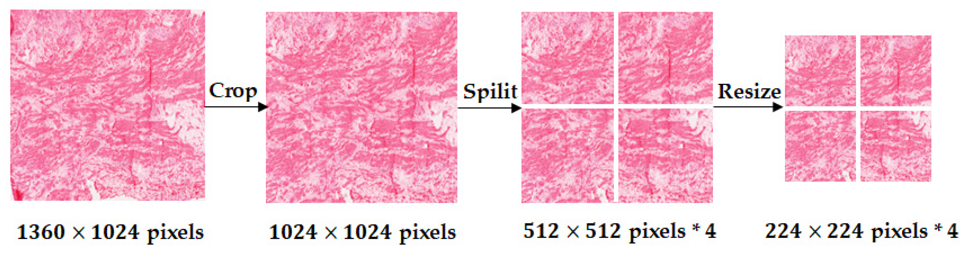
The pathological images are with high pixel characteristics and large size that cannot be directly passed as input to the CNN. In this work, image blocking is firstly implemented by cutting the full-size image to small-size images. Accordingly, all the pathology images were cropped into sub-batches with a cut size of $1024\times 1024$ pixels, each of which was then subdivided from the center point into four small images with a same size of $512\times 512$ pixels. The size of these image blocks was adjusted to $224\times 224$ pixels to fit feature extraction using CNN as demonstrated in Figure 4. The label of each batch was set as the label of the original full-size image.

3.4.2. The Structure Design of Improved CNN

Although studies have shown robustness of CNN models in various applications, the accuracy is affected by architectural factors [25,29] as kernel size ($k$), stride ($s$), padding ($p$), and number of filter channels ($f$). These hyperparameters affect the sizes of feature maps at CNN layers. So, learning time and classification accuracy are significantly influenced. Thus, this paper customizes an improved CNN model for extracting the abstract features of pathological images based on VGG16 and ALO algorithm.

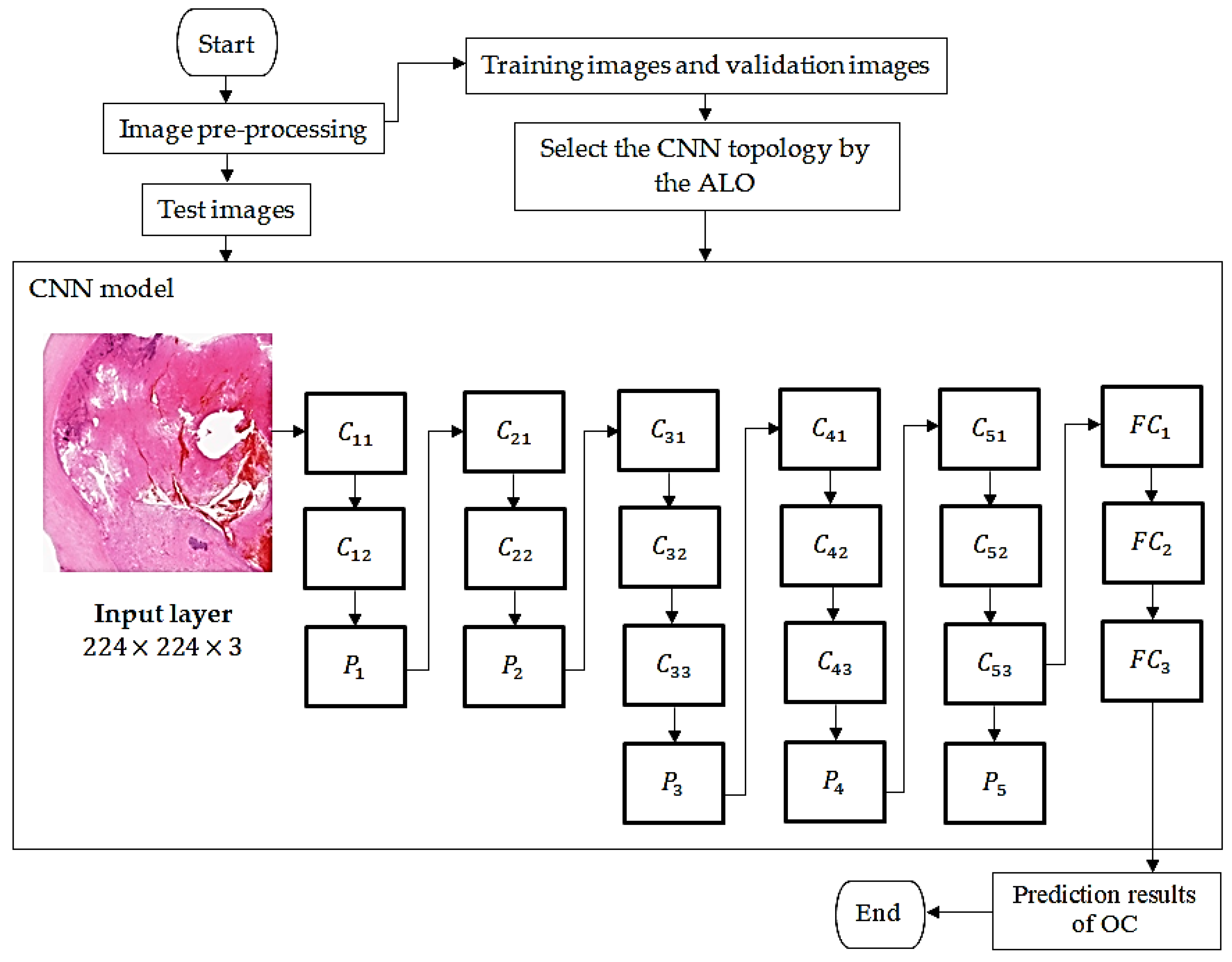
As shown in Figure 5, the structure design of the ALO-CNN model comprises the following:

Input layer: It passes the input patches into the deep network for extracting features. The network automatically adjusts the patch image to a size of $224\times 224$ to fit to the following feature extraction.

Convolutional layer: In $l th$ convolutional layer, the input batch image is subjected to a convolutional operation. Supposing $h_c$ denotes the input batch image of $l th$ convolutional layer, then a $k th$ kernel with $m\times m$ size represented by the elite is sliding across the input using stride $s$. Let $f_l$ be the number of filter channels, $w_l^{i\in f}$ and $b_l^{i\in f}$indicate the weight and bias of $i th$ filter, the output of $l th$ convolutional layer is defined using Equation (13).

$$m_l^i=\sigma \left(w_l^i-h_l+b^i\right)$$

(13)

where $\sigma$ denotes the activation function used for mapping input into nonlinear space. The output $m_l^i$ represents feature map resulted from the pathologic image. The size $d_l$ of feature map $m_l^i$ is computed using Equation (14), based on elite’s parameters, $h_l$represents input width, $k_l$ is kernel size, $p_l$ denotes padding size, and $s_l$ is stride size. Afterwards, the result (feature maps) at $lth$ convolutional layer will be activated by an activation function to get non-linear features. In this model, the ReLu [29] activation was selected by the elite, which inverses the input $x$ from negative to positive and keeps the positive values, as in Equation (15). The $\max \left(0,x\right)$ indicates ReLu function, $F\left(x\right)$is the ReLu output.

$$d_l=1+\frac{h_l-k_l+2\ast p_l}{s_l}$$

(14)

$$F\left(x\right)=\max \left(0,x\right)where\frac{\partial F\left(x\right)}{\partial x}=\{\begin{array}{c}0\\ 1\end{array}\begin{array}{c}if x\le 0\\ if x>0\end{array}$$

(15)

Pooling layer: The output feature maps are max-pooled using Equation (16), $x$ denotes the output from convolution layer, where $R_{i,j}$ denotes the $\left(i,j\right)th$ pooling region, and $P_{i,j}$ the max-pooled output.

$$P_{i,j}=\underset{r,s\in R_{i,j}}{\max }\left\{X_{r,s}\right\}$$

(16)

The best CNN topology is selected by ALO algorithm as demonstrated in

Table 3. Topology of the CNN selected by ALO.

CNN	Range/Value	Best Selected Values (Elite’s Ones)
Kernels	$\left[3–14\right]$	$k_1=4$$,k_2=3$$,k_3=8$$,k_4=7$$,k_5=7$$,k_6=3$$,k_7=5$$,k_8=3$$,k_9=3$$,k_{10}=5$$,k_{11}=3$$,k_{12}=3$$,k_{13}=4$$,k_{14}=4$$,k_{15}=5$$,k_{16}=3$$,k_{17}=8$$,k_{18}=8$.
Stride	$\left[1–5\right]$	$s_1=2$$,s_2=1$$,s_3=1$$,s_4=1$$,s_5=2$$,s_6=1$$,s_7=1$$,s_8=2$$,s_9=1$$,s_{10}=1$$,s_{11}=1$$,s_{12}=1$$,s_{13}=1$$,s_{14}=1$$,s_{15}=1$$,s_{16}=1$$,s_{17}=1$$,s_{18}=1$.
Padding	$\left[0–6\right]$	$p_1=1$$,p_2=1$$,p_3=0$$,p_4=1$$,p_5=0$$,p_6=1$$,p_7=0$$,p_8=1$$,p_9=1$$,p_{10}=0$$,p_{11}=1$$,p_{12}=0$$,p_{13}=0$$,p_{14}=1$$,p_{15}=1$$,p_{16}=0$$,p_{17}=3$$,p_{18}=3$.
Number of filters	$\left[4–15\right]$	$f_1=14$$,f_2=10$$,f_3=10$$,f_4=8$$,f_5=8$$,f_6=6$$,f_7=5$$,f_8=10$$,f_9=7$$,f_{10}=6$$,f_{11}=6$$,f_{12}=5$$,f_{13}=5$$,f_{14}=4$$,f_{15}=5$$,f_{16}=4$$,f_{17}=4$$,f_{18}=4$.
Activation function	$ReLu,Sigmoid$	$ReLu$
Pooling	$Max,Min,Average$	$Max$

. The values for the kernels of the 18 layers are $k_1=4$, $k_2=3$, $k_3=8$, $k_4=7$, $k_5=7$, $k_6=3$, $k_7=5$, $k_8=3$, $k_9=3$, $k_{10}=5$, $k_{11}=3$, $k_{12}=3$, $k_{13}=4$, $k_{14}=4$, $k_{15}=5$, $k_{16}=3$, $k_{17}=8$, $k_{18}=8$. Using unrestricted values for kernels, padding, and stride values has led to reduced dimensions of feature maps resulted at the layers of CNN, as shown in

Table 4. Dimensions of feature maps at the layers of CNN.

$C_{11}$	$C_{12}$	$P_1$	$C_{21}$	$C_{22}$
$112\times 112\times 14$	$112\times 112\times 10$	$105\times 105\times 10$	$101\times 101\times 8$	$47\times 47\times 8$
$P_2$	$C_{31}$	$C_{32}$	$C_{33}$	$P_3$
$47\times 47\times 6$	$43\times 43\times 5$	$22\times 22\times 10$	$22\times 22\times 7$	$18\times 18\times 6$
$C_{41}$	$C_{42}$	$C_{43}$	$P_4$	$C_{51}$
$18\times 18\times 6$	$16\times 16\times 5$	$15\times 15\times 5$	$14\times 14\times 4$	$12\times 12\times 5$
$C_{52}$	$C_{53}$	$P_5$	$F{C}_1 and F{C}_2$	$F{C}_3$
$12\times 12\times 4$	$11\times 11\times 4$	$10\times 10\times 4$	$1\times 1\times 120$	$1\times 1\times 84$

. Accordingly, the number of features in the last fully-connected layer is $1\times 1\times 84$ (84 features). This means that the ALO-VGG16 model returns lesser features than the original VGG16 model which returns a vector of $1\times 1\times 1000$ (1000 features).

3.5. Multimodal Fusion

The improved LSTM model extracts the features from the data of gene modality and predicts the OC stage. Similarly, the improved CNN model extracts deep-level features from the pathology images, and completes the prediction. The main idea behind the multi-modal fusion is to combine the features from different modes to distinguish the same phenomenon [12,41]. The outputs from the two network models designed in this paper are the probability distribution taken after the softmax classification [29]:

$$softmax{\left(r\right)}_j=\frac{e^{r_j}}{{\sum }_{i=1}^c{e}^{r_i}}$$

(17)

In the formula, $r_i$ indicates the data of column $i$ in the output vector, and $c$ denotes the output vector dimension. After softmax regression, the output from the network represents an $N\times 5$matrix, in which $N$ is the input samples number, and the column $j$ refers to the likelihood that the sample be in the stage $s-1$ of OC. In this study, Stage I, Stage II, Stage III, Stage IV, and Stage Not Available were labeled into class 0, class 1, class 2, class 3, class 4, and class 5, respectively. The multi-modal fusion was conducted in this work using the weighted linear aggregation, as follows:

Step 1: The trained LSTM and CNN were, respectively, implemented to validation set, where the prediction result of LSTM is $predictio{n}_{LSTM}$ and the prediction result of CNN is $predictio{n}_{CNN}$. The results from both models are $77\times 5$matrices, and 77 is the samples number included in the validation set. On the other side, for the optimized CNN model, as each sample involves many pathological image batches, we assigned the output of every sample as the average for all the sub-images of the sample.

Step 2: Fusion of the features from the two modalities was implemented using the following equation, in which the $predictio{n}_{fusion}$ indicates the feature fusion result, $\alpha$ refers to the optimized hyperparameters of LSTM modality represented by the elite, and $\beta$ denotes the optimized hyperparameters of CNN modality.

$$\begin{gathered} predictio{n}_{fusion}=\alpha .predictio{n}_{LSTM}+ \beta .predictio{n}_{CNN} \\ \{\begin{array}{c}\alpha +\beta =1\\ 0\le \alpha \le 1, 0\le \beta \le 1\end{array} \end{gathered}$$

(18)

Step 3: The best solution of $\left(\alpha , \beta \right)$ combination is transformed to the testing set, using the multi-modal features for predicting OC stage.

4. Results and Discussion

Training of the model was implemented on a laptop of Intel Core-I7 CPU. Matlab 2016A was used to implement the multi-modal fusion algorithm.

4.1. Validation Criteria

For each run of the multi-modal deep learning model, we calculated the following measures on the test data to evaluate the errors given by the classification model. The MAE [23,42] is a metric relevant to $L_1$ norm ${\parallel .\parallel }_1$ that measures average magnitude of the absolute differences between the predicted vectors $S=\left\{x_1,x_2,\dots ,x_N\right\}$ and the actual observations $S^{*}=\left\{y_1,y_2,\dots ,y_N\right\}$. Mean-Squared-Error (MSE) [42] is a metric relevant to $L_2$ norm ${\parallel .\parallel }_2$that indicates quadratic scoring rule for measuring average magnitude of the predicted vectors $S=\left\{x_1,x_2,\dots ,x_N\right\}$ and actual observations $S^{*}=\left\{y_1,y_2,\dots ,y_N\right\}$. The Mean-Absolute-Percent-Error (MAPE) and Symmetric-Mean-Absolute-Percentage-Error (SMAPE) [43], are also used which are also measures for deviation error between the predicted values $S$ and actual observations $S^{*}$, and they reveal the prediction global errors.

$${ℒ}_{MAE}\left(S,S^{*}\right)=\frac{1}{N}{\displaystyle \sum }_{k=1}^N\parallel x_k-y_k\parallel {}_1$$

(19)

$${ℒ}_{MSE}\left(S,S^{*}\right)=\frac{1}{N}{\displaystyle \sum }_{k=1}^N\parallel x_k-y_k\parallel {}_2^2$$

(20)

$$MAPE=100\times \frac{1}{N}{\displaystyle \sum }_{k=1}^N\left|\frac{x_k-y_k}{x_k}\right|$$

(21)

$$SMAPE=100\times \frac{2}{N}{\displaystyle \sum }_{k=1}^N\frac{\left|x_k-y_k\right|}{\left|x_k\right|-\left|y_k\right|}$$

(22)

So as to highlight the predictive performance of OC using the proposed multi-modal model, we use the precision $PRE$, recall $REC$, accuracy $ACC$, and F1-score for evaluation. The $TP$ denotes the number of OC positive cases predicted correctly, $FP$ indicates misclassification number in the OC positive cases, $TN$ denotes the number of OC negative cases predicted successfully, and $FN$ is misclassification number in the OC negative cases. The F1-score is utilized to make compromise between $PRE$ and $REC$.

$$PRE=\frac{TP}{TP+FP}$$

(23)

$$REC=\frac{TP}{TP+FN}$$

(24)

$$ACC=\frac{TP+TN}{TP+TN+FP+FN}$$

(25)

$$F1-\mathrm{score}=\frac{2 TP}{2 TP+FP+FN}$$

(26)

Standard deviation (SD) [40] is a statistical representation for variation in the obtained prediction results found when running the deep learning model for $k$ different runs. The SD is utilized as indicator for the stability and robustness of deep learning algorithm. The $Mean$ denotes the average performance given by the model and $o_{*}^i$ indicates the predictive result over the run $i$.

$$SD=\sqrt{\frac{1}{k-1}{\left(o_{*}^i-Mean\right)}^2}, Mean=\frac{1}{k}{\displaystyle \sum }_{i=1}^k{o}_{*}^i$$

(27)

The statistical test of Wilcoxon rank sum (W-test) [44] was also utilized to assess the performance significance, which is a non-parametric test, assigns ranks for all the scores. The W-test assigns ranks for all the scores deemed as one group, after that it sums ranks of every group. The null assumption of that two-sample test supposes the samples belong to the same population. Thus, if a difference is found in any two rank sums, it only comes from sampling error. This test is a non-parametric version of a t-test for two given independent groups. It, accordingly, tests the null assumption that the data in $i$ and $j$ vectors are samples belonging to continuous distributions of equal medians, versus the alternative assumes they are not.

4.2. Experimental Setup

In this work, each multi-modal dataset was split into: training, validation, and test sets with ratio 6:2:2.

Table 5. The samples number at each OC stage of the training, validation, and test sets.

	Stage I	Stage II	Stage II	Stage IV	Stage Not Available
Training set	11	18	268	53	3
Validation set	3	6	89	18	1
Test set	3	6	89	18	1

demonstrates the detailed data. The validation set was used to investigate the effect of hyperparameters $\left(\alpha , \beta \right)$ combination on the multi-modal fusion performance. All results were reported using the test set, and the algorithms were performed with 20 independent runs, each run has 5-fold cross validation.

4.3. Parameters Setting

The parametric setting of the ALO optimizer and the other nine compared bio-inspired algorithms is shown in

Table 6. Parameters setting for ALO and other bio-inspired algorithms.

Parameter	Setting
Maximum iterations	200
Search agents number (i.e., number of ants and antlions, wolves, colony size, whales, bats, etc.)	20
L (Controlling exploitation and exploration) for ALO	5
Crossover for GA and DE	0.5
Mutation for GA and DE	0.15
Acceleration (c1) for PSO	1.4
Acceleration (c2) for PSO	1.6
PSO maximal inertia weight	0.7
PSO minimal inertia weight	0.1
BAT constants	$f_{max}=2,f_{min}=0,\alpha =\gamma =0.9$
Random variable r for WO	[−1,1]
Logarithmic spiral shape for WO	1
Limit for ABC	5
Lower bound for GWO	−50
Upper bound for GWO	50
Flight length for CS	0.2

. The parameters of both the constructed LSTM and CNN models, which are automatically set by the ALO algorithm and the compared algorithms, were previously shown in Table 2 and Table 3.

4.4. First Experiment: Testing Proposed Model Using the OC Multi-Modal Dataset

This experiment analyzes the performance over different models established in this paper. Efficiency of the proposed multi-modal deep learning model is compared to these obtained using the single modalities: improved LSTM-based gene modality and CNN-based pathological image modality. As shown in

Table 7. Multi-modal and Single modal error evaluation and standard deviation results using the TCGA-OV dataset.

Run	Multi-Modal Fusion Model					Gene Modality					Image Modality
#	MAE	MSE	MAPE	SMAPE	SD	MAE	MSE	MAPE	SMAPE	SD	MAE	MSE	MAPE	SMAPE	SD
1	0.0215	0.1914	2.81	4.356	0.072	0.5324	0.6764	6.836	8.45	0.391	0.6642	0.7381	7.562	9.356	0.776
2	0.016	0.1613	1.362	2.284	0.013	0.5152	0.6683	6.726	8.047	0.507	0.6317	0.6147	7.275	9.099	0.347
3	0.0163	0.2344	1.764	2.731	0.019	0.4886	0.5925	6.399	7.33	0.283	0.6344	0.8547	7.333	9.12	0.861
4	0.02	0.2953	2.457	3.933	0.083	0.5005	0.6732	6.533	7.543	0.254	0.6623	0.7605	7.49	9.299	0.627
5	0.0204	0.2848	2.484	4.013	0.029	0.4999	0.5624	6.512	7.527	0.419	0.6711	0.8192	7.809	9.429	0.552
6	0.0207	0.167	2.607	4.215	0.027	0.463	0.682	6.135	7.088	0.729	0.5588	0.8317	6.88	8.686	0.702
7	0.0186	0.1208	2.253	3.609	0.096	0.5098	0.4996	6.623	7.999	0.229	0.5894	0.8857	6.988	8.813	0.551
8	0.03	0.1524	3.181	4.407	0.028	0.5248	0.4157	6.774	8.188	0.28	0.728	0.6574	8.455	10.435	0.528
9	0.0175	0.3023	2.001	3.029	0.024	0.4887	0.5997	6.419	7.432	0.641	0.6767	0.8889	7.956	9.472	0.792
10	0.0151	0.1472	1.181	1.872	0.095	0.5041	0.6166	6.552	7.609	0.167	0.6671	0.9022	7.728	9.396	0.336
11	0.0172	0.1507	1.809	2.93	0.012	0.5151	0.6046	6.678	8.014	0.18	0.5854	0.759	6.898	8.788	0.397
12	0.0206	0.26	2.595	4.081	0.032	0.4661	0.4468	6.29	7.09	0.766	0.699	0.6251	7.988	9.992	0.525
13	0.0155	0.2201	1.342	2.106	0.013	0.502	0.5957	6.549	7.572	0.162	0.6236	0.8744	7.15	8.961	0.422
14	0.0193	0.2388	2.301	3.82	0.036	0.5091	0.6209	6.619	7.918	0.317	0.8606	0.6345	8.778	10.473	0.759
15	0.0196	0.2194	2.355	3.847	0.044	0.4603	0.6429	6.077	7.066	0.388	0.6294	0.6565	7.19	8.989	0.356
16	0.0153	0.2225	1.279	1.972	0.035	0.4798	0.6991	6.342	7.111	0.414	0.6306	0.8132	7.198	9.088	0.622
17	0.0207	0.1344	2.787	4.227	0.097	0.5005	0.6988	6.533	7.543	0.348	0.6544	0.7251	7.489	9.29	0.833
18	0.0185	0.1975	2.106	3.501	0.035	0.5233	0.6322	6.753	8.154	0.699	0.6211	0.7672	7.055	8.9	0.874
19	0.0162	0.1549	1.59	2.291	0.069	0.489	0.4706	6.444	7.497	0.636	0.6476	0.8076	7.477	9.142	0.533
20	0.017	0.2942	1.771	2.888	0.017	0.5274	0.5169	6.777	8.273	0.654	0.5944	0.6544	6.999	8.859	0.607
Avg.	0.0188	0.2075	2.1018	3.3056	0.044	0.5	0.5958	6.5286	7.6726	0.424	0.6515	0.7636	7.4849	9.2794	0.6

and

Table 8. Predictive performance of the multi-modal and Single modal methods using the TCGA-OV dataset.

Run	Multi-Modal Fusion Model				Gene Modality				Image Modality
#	PRE (%)	REC (%)	ACC (%)	F1-Score	PRE (%)	REC (%)	ACC (%)	F1-Score	PRE (%)	REC (%)	ACC (%)	F1-Score
1	97.9	97.77	98	99.4	93	92.98	93.2	93.51	91.9	91.31	92	92.14
2	99	98.97	99.11	99.66	93.47	93.52	93.58	93.7	92	91.9	92.28	92.42
3	99	98.99	99.05	99.6	95	94.9	95.3	95.52	92	92.12	92.27	92.48
4	98.85	98.9	98.91	99.4	93.9	93.99	94.13	94.44	91.92	91.8	92	92.5
5	98.75	98.69	98.79	98.94	94.37	94.25	94.47	94.64	91.42	91.3	91.5	91.86
6	98.5	98.44	98.56	99.48	95.4	95.35	95.55	95.62	93.61	93.7	93.75	94
7	98.85	98.89	98.98	99.4	93.61	93.13	93.75	93.9	93	92.93	93.19	93.28
8	97.64	97.59	97.89	99.4	93.5	93.48	93.56	93.81	89.9	89.71	90	90.39
9	98.93	98.88	99	99	95	95.16	95.25	95.4	91	90.94	91.18	91.6
10	99.2	99.11	99.39	99.4	93.98	93.7	94	94.39	91.38	91.42	91.6	91.72
11	98.97	98.9	99	99.4	93.27	93.41	93.66	93.7	93	92.91	93.13	93.29
12	98.61	98.58	98.65	99.6	95.49	95.17	95.51	95.8	90.92	90.8	91	91.47
13	99.3	99	99.25	99.59	93.91	93.86	94	94.27	93	92.89	93.07	93.29
14	98.81	98.7	98.96	99.59	93	92.96	93.08	93.4	93	93.11	93.58	93.7
15	98.89	98.78	98.95	99	95.59	95.76	95.89	95.9	92.14	92	92.5	92.81
16	99	98.97	99.29	99.7	95.18	95.2	95.49	95.62	92.25	92.3	92.42	92.88
17	98.1	98	98.35	99	94.22	94	94.37	94.46	91.92	91.85	92	92.18
18	98.9	98.76	98.99	99.7	93.39	93.4	93.57	93.7	93.36	93.2	93.56	93.71
19	99	98.9	99.09	99.66	94.65	94.52	94.79	94.84	93	92.88	93.08	93.29
20	99	99.89	99.03	99.7	93	92.96	93.22	93.49	93	92.9	93.1	93.41
Avg.	98.76	98.74	98.87	99.43	94.15	94.09	94.32	94.51	92.19	92.1	92.37	92.63

, the proposed deep learning model by amalgamating heterogeneous features of genomic data and pathological images realizes the lowest MAE, MSE, MAPE, and SMAPE. The obtained error rates are 0.0188, 0.2075, 2.1018, and 3.3056, respectively. The proposed model also shows the lowest SD value (0.044) over the 20 runs, which reveals its stability and robustness. On the other hand, it shows the best predictive performance with regard to precision, recall, accuracy, and F1-score. The given results are 98.76, 98.74, 98.87, and 99.43%, respectively. It is also observed that the gene modality model comes in the second rank after the proposed model in terms of error evaluation rates, predictive performance, and SD value. The potential reason for that optimization is that genomic data can effectively reflect the OC characteristics, so feature learning by using only image level is not enough to realize the high-performance requirements.

4.5. Second Experiment: Testing Proposed Model Using Benchmarks for Other Cancers

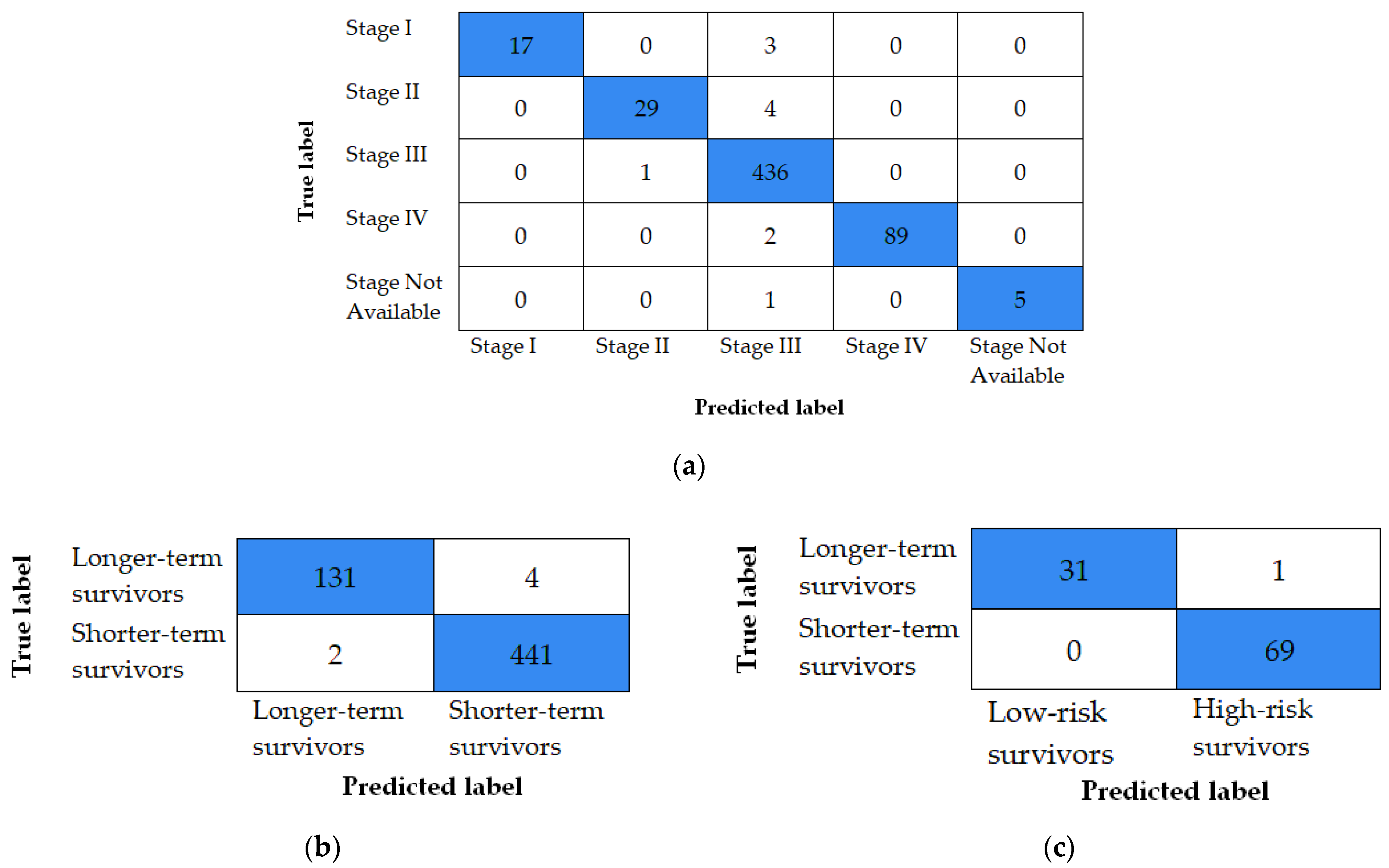
In this experiment, we evaluate our multi-modal fusion framework on two benchmarks for other cancers taken from the TCGA. The first dataset is Breast Invasive Carcinoma (BRCA) [9,10] that includes histopathology images alongside with genomic profiling reports for 578 cases. Among them, 133 cases are labeled as longer-term survivors and 445 cases are labeled as shorter-term survivors. The second dataset is Lung Squamous Cell Carcinoma, (LUSC) [10,11], which involves 101 cases, 31 patients of them are classified as low-risk survivors, and 70 patients are classified as high-risk survivors. The performance is assessed through various ways. Here, confusion matrix is utilized, which provides valuable information on the predicted and actual labels given by the proposed fusion method. By using that information, the performance can be evaluated from different aspects, as seen in Figure 6 which shows the confusion matrix for BRCA and LUSC datasets versus the TCGA-OV dataset. The diagonal blue-shadowed numbers represent the true positives of cancer class, while the white-shadowed numbers represent the confused false positives. Clearly, we observe that the proposed multi-modal fusion algorithm improved accuracy of each cancer recognition system by significant amount, through increasing the number of true positives and reducing the number of false positives, over each dataset.

From

Table 9. Error evaluation and prediction results of the multi-modal and single modal approaches using benchmarks for other cancers.

Dataset	MAE	MSE	MAPE	SMAPE	SD	PRE (%)	REC (%)	ACC (%)	F1-Score (%)
BRCA	0.0155	0.1254	2.115	3.347	0.047	98.35	98.42	98.8	98.92
LUSC	0.0139	0.1066	2.1	3.299	0.029	98.78	98.71	99.28	99.31
BRCA (Image modal)	0.5784	0.8661	7.122	9.503	0.337	92.88	93	93.19	93.4
BRCA (Gene modal)	0.5004	0.5798	6.567	7.976	0.243	93.94	94.22	94.49	94.52
LUSC (Image modal)	0.5661	0.7898	6.923	8.917	0.299	92.96	93.11	93.31	93.49
LUSC (Gene modal)	0.4886	0.5511	5.991	7.443	0.205	94.17	94.7	94.76	94.9

, we can also derive that for the BRCA and LUSC benchmarks, the proposed model realizes more accurate discriminative results than the single gene modal and histopathology image modal. The accuracy is 98.8 and 99.28%, while the F-score is 98.92 and 99.31%, respectively. The obtained MAE rate is 0.0155 and 0.0139, while the MSE is 0.1254 and 0.1066, and the SD value is 0.047 and 0.029, respectively, which are lower than these of the compared single modalities.

Furthermore, for each benchmark, the significance of performance is also assessed using the Wilcoxon test and the results are shown in

Table 10. Wilcoxon test results across all the benchmarks.

Dataset	Gene Modality	Image Modality
TCGA-OV	0.024	0.039
BRCA	0.033	0.044
LUSC	0.022	0.049

. The table demonstrates that across all the datasets, the proposed model has significant difference over all the compared single modalities, which means that it reveals significant enhance over all these models at (0.05) significance level. These results obviously reflect that the integrative analysis for both pathological images and genomic data using the proposed multi-modal fusion model can also efficiently improve the predictive performance of breast and lung cancers, which indicates that the proposed model is applicable to the other cancers.

4.6. Comparative Analysis

Extensive experiments were conducted to assess the performance of proposed multi-modal fusion model (with) and without the optimization algorithms, by using the three benchmarks. Accordingly, we evaluate the effect of the topology of LSTM and CNN models selected by different bio-inspired optimization algorithms on the error reduction and predictive performance of the model. The compared state-of-the-art algorithms include the GA [35], PSO [33], DE [30], GWO [26], ABC [29], WO [31], CS algorithm [28], and BAT algorithm [34]. By comparing the prediction ability of the proposed model to these obtained by the other nine models established using the compared bio-inspired algorithms shown in

Table 11. Evaluation results given by each one of the nine constructed multi-modal fusion models over the three datasets.

Dataset	Measure	ALO (ours)	No Opt.	GA	PSO	DE	BAT	ABC	WO	GWO	CS
TCGA-OV	MAE	0.0188	0.9854	0.4693	0.4324	0.4161	0.3479	0.2453	0.1974	0.158	0.0779
	MSE	0.2075	1.1523	0.6237	0.6001	0.6	0.5721	0.4609	0.3055	0.2433	0.2309
	MAPE	2.1018	9.746	5.819	5.404	4.765	4.101	3.746	3.112	2.908	2.632
	SMAPE	3.3056	11.485	6.05	5.899	4.966	4.119	3.882	3.682	3.499	3.329
	SD	0.044	0.831	0.654	0.537	0.519	0.501	0.374	0.331	0.298	0.249
	PRE (%)	98.76	93.11	95	95.44	95.98	96.31	96.77	96.9	97.34	97.77
	REC (%)	98.74	93.39	95.25	95.63	96.21	96.54	96.97	97.11	97.69	97.8
	ACC (%)	98.87	93.7	95.38	95.91	96.39	96.66	96.84	97.14	97.42	97.91
	F1-score (%)	99.43	93.89	95.48	95.99	96.42	96.81	96.92	97.25	97.58	97.96
	W-test			0.0444	0.0433	0.0411	0.0407	0.0394	0.0321	0.0066	0.0022
BRCA	MAE	0.0155	0.9949	0.4801	0.3001	0.241	0.1982	0.1112	0.0881	0.0762	0.0552
	MSE	0.1254	1.2372	0.7723	0.6934	0.6401	0.6012	0.5222	0.4179	0.3499	0.3195
	MAPE	2.115	9.823	5.909	4.055	3.85	3.24	2.97	2.75	2.44	2.211
	SMAPE	3.347	11.66	6.221	5.112	4.772	3.988	3.715	3.526	3.349	3.33
	SD	0.047	0.903	0.725	0.641	0.6	0.559	0.416	0.338	0.31	0.306
	PRE (%)	98.35	92.66	95.32	95.95	96.23	96.63	96.97	97.84	97.67	98.13
	REC (%)	98.42	93.51	95.29	96	96.11	96.8	97	97.89	97.91	98.35
	ACC (%)	98.8	93	95.18	96.37	96.68	96.75	97.04	97.35	97.7	97.95
	F1-score (%)	98.92	92.87	94.39	96.43	96.75	96.89	97.1	97.5	97.81	97.98
	W-test			0.043	0.0424	0.0415	0.0402	0.0338	0.0323	0.0218	0.0216
LUSC	MAE	0.0139	0.8341	0.3942	0.2998	0.2112	0.1361	0.0997	0.0551	0.0485	0.0391
	MSE	0.1066	0.9907	0.6893	0.5875	0.4933	0.4221	0.3779	0.3055	0.3	0.2989
	MAPE	2.1	8.542	4.286	3.993	3.49	3.09	2.913	2.591	2.442	2.29
	SMAPE	3.299	10.33	5.27	4.879	4.611	4.432	3.992	3.771	3.566	3.439
	SD	0.029	0.799	0.645	0.613	0.59	0.513	0.375	0.327	0.302	0.295
	PRE (%)	98.78	93.45	95.61	96.14	96.39	96.88	97.19	97.92	98.11	98.25
	REC (%)	98.71	94. 62	96.4	96.2	96.21	96.9	97.29	97.83	97.95	98.3
	ACC (%)	99.28	93.91	96	96.41	96.67	96.78	97.17	97.59	97.83	97.97
	F1-score (%)	99.31	93.52	96.05	96.54	96.77	96.92	97.13	97.69	97.92	98
	W-test			0.0425	0.0419	0.0402	0.0345	0.0336	0.0251	0.0221	0.0019

, we can realize that across the three datasets, the proposed model achieved the highest precision, recall, accuracy, and F-score, with limited error rates and low SD values. In terms of Wilcoxon test, it also has significance difference against the other constructed bio-inspired deep learning models, at significance level of 0.05. Furthermore, models based on CS, GWO, and WO ranked as second, third, and fourth, respectively, with regard to OC stage prediction. It is also noted that the model constructed for the diagnosis using only the two deep feature extractors without bio-inspired optimization has shown lower performance in comparison to the other evolutionary multi-modal deep learning models or even the other evolutionary single modal deep learning models. This reflects the high impact of the model construction on the deep learning performance.

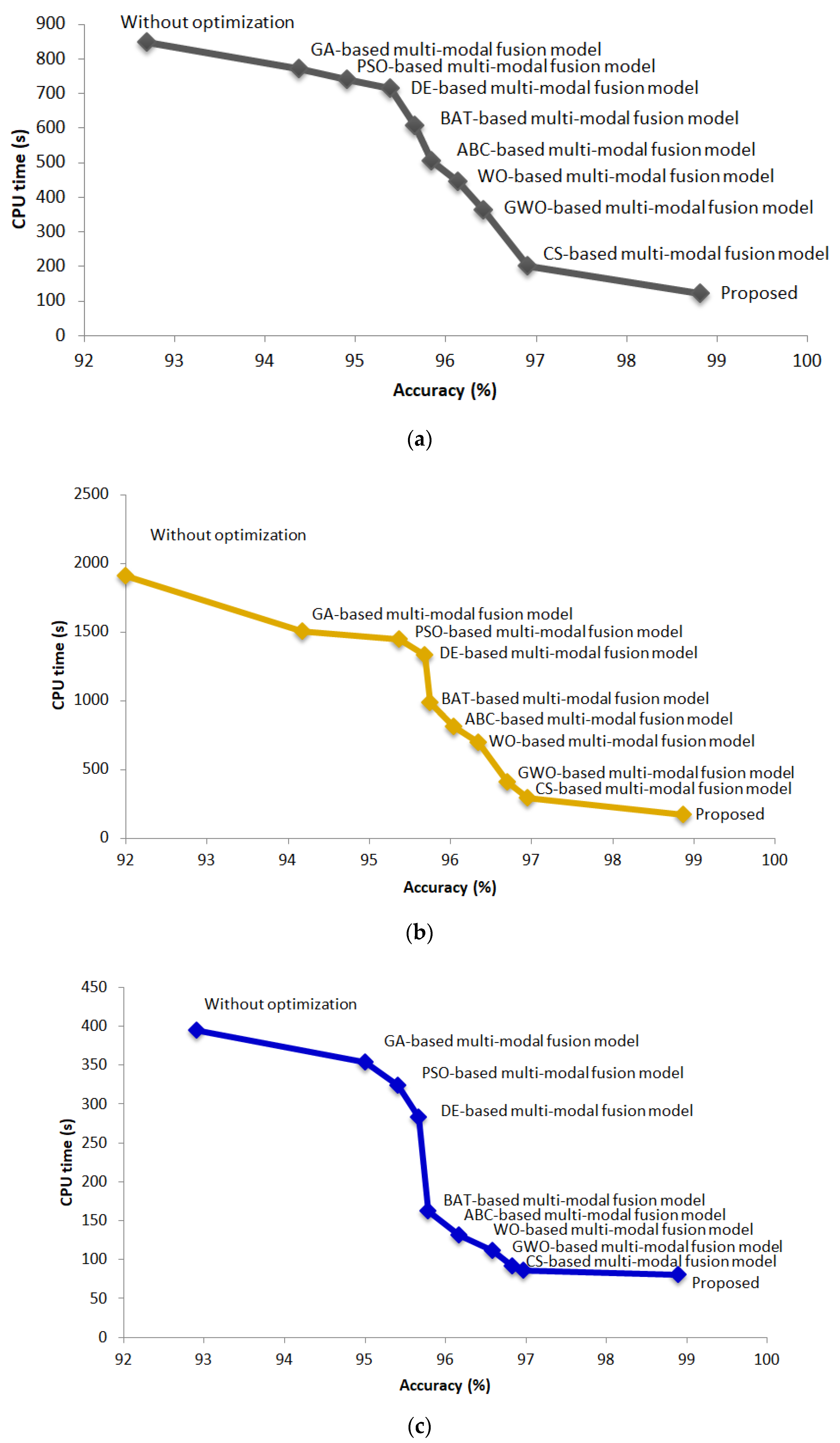
The convergence speed curves of all the constructed multi-modal fusion models using the TCGA-OV, BRCA, and LUSC datasets are presented in Figure 7, respectively, which demonstrates how the fitness decreases over the iterations and proves that the ALO escapes local minima in the three multi-modal datasets and is capable of finding the optimal combination of LSTM and CNN weights that improves the fusion results in less than 10 iterations. Furthermore, the proposed model achieved optimal prediction accuracy in a shorter computational time across the three datasets. Average CPU time of roughly 120.6, 173.4, and 80.8 s has been taken across the whole dataset, respectively, while the best and worst computed fitness yielded by the model across each dataset were ≈0.08 and ≈0.09, respectively, as demonstrated in Figure 8.

So as to discuss the rationality of CNN constructed in this work for pathology image feature extraction, and investigate the advantages of VGG16 infrastructure optimized with ALO algorithm, we replace the VGG16 architecture with the AlexNet [45] and ResNet34 [45], and do some comparisons. In this context, the ALO algorithm was used to set the topology of each network model. It is clearly noted from

Table 12. Comparison of the VGG16 performance against different CNNs.

Measure	TCGA-OV			BRCA			LUSC
	ResNet34	AlexNet	Proposed	ResNet34	AlexNet	Proposed	ResNet34	AlexNet	Proposed
MAE	0.5975	0.6009	0.0188	0.5375	0.6682	0.0155	0.5006	0.6552	0.0139
MSE	0.7752	0.8211	0.2075	0.7245	0.8014	0.1254	0.5114	0.7716	0.1066
MAPE	5.705	6.101	2.1018	5.001	5.884	2.115	4.883	5.737	2.1
SMAPE	4.119	5.711	3.3056	6.112	6.501	3.347	4.937	5.992	3.299
SD	0.681	0.724	0.044	0.596	0.649	0.047	0.515	0.607	0.029
PRE (%)	96.6	96	98.76	96.98	96.3	98.35	96.78	96.25	98.78
REC (%)	96.9	96.4	98.74	96.27	96.11	98.42	96.93	96	98.71
ACC (%)	96.55	95.95	98.87	96.81	95.63	98.8	96.97	95.88	99.28
F1-score (%)	97.7	96.19	99.43	97.1	95.8	98.92	97.14	96.1	99.31
W-test	0.037	0.04		0.041	0.045		0.0341	0.0417
CPU Time	205.02 s	276.88 s	120.6 s	236.98 s	296.52	173.4 s	121.2 s	185.04 s	80.8 s

that the accuracy based upon the ResNet34 is 96.55, 96.81, and 96.97% on TCGA-OV, BRCA, and LUSC, respectively, while the accuracy based upon the AlexNet is 95.95, 95.63, and 95.88%, respectively. These accuracies are lower in comparison to the VGG16. Additionally, the ResNet34 model outperforms the AlexNet model in terms of predictive performance, error rate, and SD value. Furthermore, the CPU time taken by using the proposed model was smaller than the two other models over the three datasets. There is also significant difference at 0.05-level for the VGG16 model against the two other models in terms of Wilcoxon test.

4.7. Comparisons to Others

To further verify the efficiency of the proposed multi-modal fusion model for cancer diagnosis from multi-modal data, we compared it to the recent works that used the same multi-modal benchmarks used in this work.

Table 13. Comparison between the proposed multi-modal fusion model and the state-of-the-art models.

Ref.	Dataset	Performance Measure
		AUC	ACC (%)	PRE (%)	REC (%)	F1-Score (%)
[6]	TCGA-OV	0.95	-	-	-	-
[9]	BRCA	0.828	80.22	63.4	28.5	-
[10]	BRCA	-	72.53	78.76	88.18	83.17
	LUSC	-	70.08	73.57	81.25	77.49
[11]	LUSC	0.8793	80.22	81.25	57.14	-
[12]	BRCA	0.9427	88.07	-	-	-
Proposed	TCGA-OV	-	98.87	98.5	98.89	99.43
	BRCA	-	98.8	98.35	99	99.4
	LUSC	-	99.28	98.78	99.25	99.64

[6,9,10,11,12] illustrates the comparison. For instance, Yu et al. [6] presented a single modal approach based on analysis of the whole-slide pathology images from 587 primary serous ovarian adenocarcinoma patients taken from the TCGA. The CNNs were used to classify the pathology images with cancerous cells, predict the pathology grade of the OC patient, and predict platinum-based chemotherapy. The area under the receiver-operating-characteristic curve (AUC) was 0.95 for classification of cancerous regions and 0.80 for classification of tumor grade. The “inverted pyramid” deep neural network and VGG16 were the methods used by Liu et al. [12] to, respectively, extract gene features and pathological image features of breast cancer. The multi-modal fusion was implemented using weighted linear aggregation and simulated annealing algorithm.

In summary, the multi-modal fusion model established in this work was superior to the other models with regard to various indicators. There are multiple factors for why the proposed model performs well in diagnosis of OC and other cancers. First, combining heterogeneous features of genomic data and pathology images can consistently achieve robust and accurate diagnosis results than the single modal diagnosis. Second, the traditional ML and CNNs models still lack to the optimization of the model construction in the domain of cancer subtypes. We present a flexible designed ALO-LSTM gene feature extraction network, which does not suppose fixed topology, for example, the input length and number of LSTM units need in the sequential processing of gene data is selected by the ALO. The established network was stable in processing the gene features for a short or a long interval of time without causing vanishing gradient. Additionally, the improved ALO-CNN pathological feature extraction network does not suppose fixed size for kernels, filters, strides, and padding values. This helped to provide the most informative features from the two modalities and improved the diagnosis results.

5. Conclusions

This paper works to overcome the potential insufficient representation of OC characteristics caused by the single modal approaches used previously in the state-of-the-art by proposing a multi-modal deep learning model in order to precisely predict OC stage. The model combines gene modality along with histopathology image modality. So it is composed of two evolutionary deep-feature extraction network models. The first one is a predictive ALO-optimized LSTM network to sequentially process the longitudinal data of gene modality while the second is a predictive ALO-optimized CNN for extracting the abstract features from pathological images. In this context, the ALO optimizer is hybridized with each feature network to automatically set its topology, which helped to diminish the model’s errors and increase predictive accuracy of OC stage. Then, the deep features from the two improved networks are fused based upon weighted linear aggregation. The experimental results were conducted using a public multi-modal OC dataset and two benchmarks for other cancers. The results revealed that the proposed multi-modal fusion model by amalgamating heterogeneous features, including genomic and image information, realizes optimal accuracy and lower error rates than those models comprising single modal data. After that, extensive comparisons have been made using each multi-modal dataset for assessing the performance based on various recent bio-inspired optimization algorithms. Among the compared models, the proposed model achieved not only the highest prediction accuracy and lowest classification error but also the highest convergence speed and shortest CPU time over all the multi-modal datasets. Furthermore, the proposed model shows significant difference against all the models constructed in this paper in terms of Wilcoxon test. These results are due to the stability and robustness of the ALO-LSTM network in extracting genomic features from the gene modal data for a short or a long interval of time without causing vanishing gradient. In addition to the flexibility of ALO-CNN network which does not consider static values for kernels, padding, and filter channels. This made the network extract the sufficient abstract features from the pathological images and discard the useless ones, in addition to the higher exploitation and convergence speed of the ALO algorithm in providing the best topology for each feature network in a way that optimized the prediction results of OC and other cancers. In the future work, we intend to amalgamate different modalities to deeply predict other diseases including respiratory system disease.

References

- Vázquez, M.A.; Mariño, I.P.; Blyuss, O.; Ryan, A.; Gentry-Maharaj, A.; Kalsi, J.; Manchanda, R.; Jacobs, I.; Menon, U.; Zaikin, A. A quantitative performance study of two automatic methods for the diagnosis of ovarian cancer. Biomed. Signal Process. Control 2018, 46, 86–93. [Google Scholar] [CrossRef] [PubMed]
- Jayson, G.C.; Kohn, E.C.; Kitchener, H.C.; Ledermann, J.A. Ovarian cancer. Lancet 2014, 384, 1376–1388. [Google Scholar] [CrossRef]
- Kommoss, S.; Pfisterer, J.; Reuss, A.; Diebold, J.; Hauptmann, S.; Schmidt, C.; Bois, A.D.; Schmidt, D.; Kommoss, F. Specialized Pathology Review in Patients with Ovarian Cancer. Int. J. Gynecol. Cancer 2013, 23, 1376–1382. [Google Scholar] [CrossRef]
- Bentaieb, A.; Li-Chang, H.; Huntsman, D.; Hamarneh, G. Automatic Diagnosis of Ovarian Carcinomas via Sparse Multiresolution Tissue Representation. In Lecture Notes in Computer Science Medical Image Computing and Computer-Assisted Intervention—MICCAI 2015; Springer: Berlin, Germany, 2015; pp. 629–636. [Google Scholar]
- Bentaieb, A.; Li-Chang, H.; Huntsman, D.; Hamarneh, G. A structured latent model for ovarian carcinoma subtyping from histopathology slides. Med. Image Anal. 2017, 39, 194–205. [Google Scholar] [CrossRef] [PubMed]
- Yu, K.-H.; Hu, V.; Wang, F.; Matulonis, U.A.; Mutter, G.L.; Golden, J.A.; Kohane, I.S. Deciphering serous ovarian carcinoma histopathology and platinum response by convolutional neural networks. BMC Med. 2020, 18. [Google Scholar] [CrossRef] [PubMed]
- Papp, E.; Hallberg, D.; Konecny, G.E.; Bruhm, D.C.; Adleff, V.; Noë, M.; Kagiampakis, I.; Palsgrove, D.; Conklin, D.; Kinose, Y.; et al. Integrated Genomic, Epigenomic, and Expression Analyses of Ovarian Cancer Cell Lines. Cell Rep. 2018, 25, 2617–2633. [Google Scholar] [CrossRef] [PubMed] [Green Version]
- Integrated genomic analyses of ovarian carcinoma. Nature 2011, 474, 609–615.
- Sun, D.; Li, A.; Tang, B.; Wang, M. Integrating genomic data and pathological images to effectively predict breast cancer clinical outcome. Comput. Methods Programs Biomed. 2018, 161, 45–53. [Google Scholar] [CrossRef] [PubMed]
- Shao, W.; Wang, T.; Sun, L.; Dong, T.; Han, Z.; Huang, Z.; Zhang, J.; Zhang, D.; Huang, K. Multi-task multi-modal learning for joint diagnosis and prognosis of human cancers. Med. Image Anal. 2020, 65, 101795. [Google Scholar] [CrossRef] [PubMed]
- Zhang, A.; Li, A.; He, J.; Wang, M. LSCDFS-MKL: A multiple kernel based method for lung squamous cell carcinomas disease-free survival prediction with pathological and genomic data. J. Biomed. Inform. 2019, 94, 103194. [Google Scholar] [CrossRef]
- Liu, T.; Huang, J.; Liao, T.; Pu, R.; Liu, S.; Peng, Y. A Hybrid Deep Learning Model for Predicting Molecular Subtypes of Human Breast Cancer Using Multimodal Data. Irbm 2021. [Google Scholar] [CrossRef]
- Kott, O.; Linsley, D.; Amin, A.; Karagounis, A.; Jeffers, C.; Golijanin, D.; Serre, T.; Gershman, B. Development of a Deep Learning Algorithm for the Histopathologic Diagnosis and Gleason Grading of Prostate Cancer Biopsies: A Pilot Study. Eur. Urol. Focus 2019, 7, 347–351. [Google Scholar] [CrossRef] [PubMed] [Green Version]
- Ismael, S.A.A.; Mohammed, A.; Hefny, H. An enhanced deep learning approach for brain cancer MRI images classification using residual networks. Artif. Intell. Med. 2020, 102, 101779. [Google Scholar] [CrossRef] [PubMed]
- Harangi, B.; Baran, A.; Hajdu, A. Assisted deep learning framework for multi-class skin lesion classification considering a binary classification support. Biomed. Signal. Process. Control 2020, 62, 102041. [Google Scholar] [CrossRef]
- Celik, Y.; Talo, M.; Yildirim, O.; Karabatak, M.; Acharya, U.R. Automated invasive ductal carcinoma detection based using deep transfer learning with whole-slide images. Pattern Recognit. Lett. 2020, 133, 232–239. [Google Scholar] [CrossRef]
- Guo, D.; Duan, G.; Yu, Y.; Li, Y.; Wu, F.-X.; Li, M. A disease inference method based on symptom extraction and bidirectional Long Short Term Memory networks. Methods 2020, 173, 75–82. [Google Scholar] [CrossRef] [PubMed]
- Datta, S.; Si, Y.; Rodriguez, L.; Shooshan, S.E.; Demner-Fushman, D.; Roberts, K. Understanding spatial language in radiology: Representation framework, annotation, and spatial relation extraction from chest X-ray reports using deep learning. J. Biomed. Inform. 2020, 108, 103473. [Google Scholar] [CrossRef] [PubMed]
- Gao, R.; Huo, Y.; Bao, S.; Tang, Y.; Antic, S.L.; Epstein, E.S.; Balar, A.B.; Deppen, S.; Paulson, A.B.; Sandler, K.L.; et al. Distanced LSTM: Time-Distanced Gates in Long Short-Term Memory Models for Lung Cancer Detection. In Machine Learning in Medical Imaging Lecture Notes in Computer Science; Springer: Berlin, Germany, 2019; pp. 310–318. [Google Scholar]
- Lu, Z.; Pu, H.; Wang, F.; Hu, Z.; Wang, L. The expressive power of neural networks: A view from the width. Proc. Adv. Neural Inf. Process. Syst. 2017, 6231–6239. Available online: https://arxiv.org/abs/1709.02540 (accessed on 2 March 2021).
- Rolnick, D.; Tegmark, M. The power of deeper networks for expressing natural functions. In Proceedings of the International Conference on Learning Representations, Vancouver, BC, Canada, 30 April–3 May 2018. [Google Scholar]
- Du, S.; Lee, J. On the power of over-parametrization in neural networks with quadratic activation. In Proceedings of the 35th International Conference on Machine Learning (ICML), Stockholm, Sweden, 10–15 July 2018; Volume 80, pp. 1329–1338. [Google Scholar]
- Qi, J.; Du, J.; Siniscalchi, S.M.; Ma, X.; Lee, C.-H. Analyzing Upper Bounds on Mean Absolute Errors for Deep Neural Network-Based Vector-to-Vector Regression. IEEE Trans. Signal. Process. 2020, 68, 3411–3422. [Google Scholar]
- Liu, P.; Basha, M.D.E.; Li, Y.; Xiao, Y.; Sanelli, P.C.; Fang, R. Deep Evolutionary Networks with Expedited Genetic Algorithms for Medical Image Denoising. Med. Image Anal. 2019, 54, 306–315. [Google Scholar] [CrossRef]
- Gao, Z.; Li, Y.; Yang, Y.; Wang, X.; Dong, N.; Chiang, H.-D. A GPSO-optimized convolutional neural networks for EEG-based emotion recognition. Neurocomputing 2020, 380, 225–235. [Google Scholar] [CrossRef]
- Samuel, O.D.; Okwu, M.O.; Oyejide, O.J.; Taghinezhad, E.; Afzal, A.; Kaveh, M. Optimizing biodiesel production from abundant waste oils through empirical method and grey wolf optimizer. Fuel 2020, 281, 118701. [Google Scholar] [CrossRef]
- Dalwinder, S.; Birmohan, S.; Manpreet, K. Simultaneous feature weighting and parameter determination of Neural Networks using Ant Lion Optimization for the classification of breast cancer. Biocybern. Biomed. Eng. 2020, 40, 337–351. [Google Scholar] [CrossRef]
- Gupta, D.; Sundaram, S.; Khanna, A.; Hassanien, A.E.; Albuquerque, V.H.C.D. Improved diagnosis of Parkinsons disease using optimized crow search algorithm. Comput. Electr. Eng. 2018, 68, 412–424. [Google Scholar] [CrossRef]
- Ghoniem, R.M. A Novel Bio-Inspired Deep Learning Approach for Liver Cancer Diagnosis. Information 2020, 11, 80. [Google Scholar] [CrossRef] [Green Version]
- Özyön, S. Optimal short-term operation of pumped-storage power plants with differential evolution algorithm. Energy 2020, 194, 116866. [Google Scholar] [CrossRef]
- Ghoniem, R.M.; Alhelwa, N.; Shaalan, K. A Novel Hybrid Genetic-Whale Optimization Model for Ontology Learning from Arabic Text. Algorithms 2019, 12, 182. [Google Scholar] [CrossRef] [Green Version]
- Penghui, L.; Ewees, A.A.; Beyaztas, B.H.; Qi, C.; Salih, S.Q.; Al-Ansari, N.; Bhagat, S.K.; Yaseen, Z.M.; Singh, V.P. Metaheuristic Optimization Algorithms Hybridized with Artificial Intelligence Model for Soil Temperature Prediction: Novel Model. IEEE Access 2020, 8, 51884–51904. [Google Scholar] [CrossRef]
- Ghoniem, R.M.; Shaalan, K. FCSR—Fuzzy Continuous Speech Recognition Approach for Identifying Laryngeal Pathologies Using New Weighted Spectrum Features. In Proceedings of the International Conference on Advanced Intelligent Systems and Informatics 2017 Advances in Intelligent Systems and Computing, Cairo, Egypt, 9–11 September 2017; Springer: Berlin, Germany, 2017; pp. 384–395. [Google Scholar]
- Dong, J.; Wu, L.; Liu, X.; Li, Z.; Gao, Y.; Zhang, Y.; Yang, Q. Estimation of daily dew point temperature by using bat algorithm optimization based extreme learning machine. Appl. Therm. Eng. 2020, 165, 114569. [Google Scholar] [CrossRef]
- Velliangiri, S.; Karthikeyan, P.; Xavier, V.A.; Baswaraj, D. Hybrid electro search with genetic algorithm for task scheduling in cloud computing. Ain Shams Eng. J. 2020, 12, 631–639. [Google Scholar] [CrossRef]
- Banerjee, I.; Ling, Y.; Chen, M.C.; Hasan, S.A.; Langlotz, C.P.; Moradzadeh, N.; Chapman, B.; Amrhein, T.; Mong, D.; Rubin, D.L.; et al. Comparative effectiveness of convolutional neural network (CNN) and recurrent neural network (RNN) architectures for radiology text report classification. Artif. Intell. Med. 2019, 97, 79–88. [Google Scholar] [CrossRef] [PubMed]
- Ali, E.; Elazim, S.A.; Abdelaziz, A. Ant Lion Optimization Algorithm for Renewable Distributed Generations. Energy 2016, 116, 445–458. [Google Scholar] [CrossRef]
- Peng, L.; Liu, S.; Liu, R.; Wang, L. Effective long short-term memory with differential evolution algorithm for electricity price prediction. Energy 2018, 162, 1301–1314. [Google Scholar] [CrossRef]
- Mirjalili, S. The Ant Lion Optimizer. Adv. Eng. Softw. 2015, 83, 80–98. [Google Scholar] [CrossRef]
- Emary, E.; Zawbaa, H.M.; Hassanien, A.E. Binary ant lion approaches for feature selection. Neurocomputing 2016, 213, 54–65. [Google Scholar] [CrossRef]
- Ghoniem, R.M.; Algarni, A.D.; Shaalan, K. Multi-Modal Emotion Aware System Based on Fusion of Speech and Brain Information. Information 2019, 10, 239. [Google Scholar] [CrossRef] [Green Version]
- Qi, J.; Du, J.; Siniscalchi, S.M.; Ma, X.; Lee, C.-H. On Mean Absolute Error for Deep Neural Network Based Vector-to-Vector Regression. IEEE Signal. Process. Lett. 2020, 27, 1485–1489. [Google Scholar] [CrossRef]
- Cen, Z.; Wang, J. Crude oil price prediction model with long short term memory deep learning based on prior knowledge data transfer. Energy 2019, 169, 160–171. [Google Scholar] [CrossRef]
- Wilcoxon, F. Individual Comparisons by Ranking Methods. Biom. Bull. 1945, 1, 80. [Google Scholar] [CrossRef]
- Zarie, M.; Jahedsaravani, A.; Massinaei, M. Flotation froth image classification using convolutional neural networks. Miner. Eng. 2020, 155, 106443. [Google Scholar]
Figure 1.
Basic architecture of (a) convolutional neural network, and (b) LSTM.
Figure 2.
Workflow of the proposed multi-modal fusion model.
Figure 3.
A flowchart of the ALO-optimized LSTM network constructed for feature extraction from the gene modal data.
Figure 4.
Pre-processing of the pathology images.
Figure 5.
A flowchart of the ALO-CNN network constructed for feature extraction from the pathology image modality.
Figure 6.
Confusion matrix for (a) TCGA-OV dataset, (b) BRCA dataset, and (c) LUSC dataset.
Figure 7.
Convergence curves of all the constructed multi-modal fusion models on the (a) TCGA-OV dataset, (b) BRCA dataset, and (c) LUSC dataset.
Figure 8.
CPU time versus accuracy for all algorithms on the (a) TCGA-OV, (b) BRCA, and (c) LUSC.