Measurement of the Casimir Force between 0.2 and 8 μm: Experimental Procedures and Comparison with Theory

Abstract

We present results on the determination of the differential Casimir force between an Au-coated sapphire sphere and the top and bottom of Au-coated deep silicon trenches performed by means of the micromechanical torsional oscillator in the range of separations from 0.2 to 8 $\mathsf{\mu }$m. The random and systematic errors in the measured force signal are determined at the 95% confidence level and combined into the total experimental error. The role of surface roughness and edge effects is investigated and shown to be negligibly small. The distribution of patch potentials is characterized by Kelvin probe microscopy, yielding an estimate of the typical size of patches, the respective r.m.s. voltage and their impact on the measured force. A comparison between the experimental results and theory is performed with no fitting parameters. For this purpose, the Casimir force in the sphere-plate geometry is computed independently on the basis of first principles of quantum electrodynamics using the scattering theory and the gradient expansion. In doing so, the frequency-dependent dielectric permittivity of Au is found from the optical data extrapolated to zero frequency by means of the plasma and Drude models. It is shown that the measurement results exclude the Drude model extrapolation over the region of separations from 0.2 to 4.8 $\mathsf{\mu }$m, whereas the alternative extrapolation by means of the plasma model is experimentally consistent over the entire measurement range. A discussion of the obtained results is provided.

1. Introduction

The Casimir attraction [1] between two uncharged closely spaced bodies is a macroscopic quantum effect which is caused by the zero-point and thermal fluctuations of the electromagnetic field. Over a long period of time, it was measured only up to an order of magnitude. The modern period in experimental investigation of this phenomenon started from measuring the Casimir force between the Au-coated surfaces of a large lens and a plate by means of the torsion pendulum [2]. Precise measurements of the Casimir force have been made possible only during the last 20 years thanks to microtechnology achievements. These measurements gave the possibility of quantitatively checking the theoretical predictions of the Lifshitz theory [3,4] which generalizes the original Casimir prediction (made for two parallel ideal metal planes at zero temperature) for the case of thick plates described by their frequency-dependent dielectric permittivities in thermal equilibrium with the environment.

The first experiment of this kind used an atomic force microscope where the sharp tip was replaced with the sphere of about 100 $\mathsf{\mu }$m radius [5]. This experiment made it possible to demonstrate corrections to the famous Casimir expression due to the finite conductivity of the boundary metal. Another novel facility of nanotechnology, a micromechanical torsional oscillator, was used to demonstrate the actuation of micromechanical devices by the Casimir force [6,7]. After experimental improvements [8], micromechanical torsional oscillators were used in the most precise measurements of the Casimir interaction between an Au-coated sapphire sphere of 150 $\mathsf{\mu }$m radius and an Au-coated polysilicon plate [9,10,11,12].

It turned out that the theoretical predictions of the Lifshitz theory are excluded by the measurement data [9,10,11,12] if the dielectric permittivity is obtained from the measured optical data of Au [13] extrapolated down to zero frequency by means of the dissipative Drude model which takes the proper account of the relaxation properties of conduction electrons. The Lifshitz theory using the Drude model was excluded over the separation region from 160 to 750 nm. What is even more surprising, an agreement between experiment and theory was restored [9,10,11,12] if, except of the Drude model, an extrapolation was made using the dissipationless plasma model which disregards the relaxation properties of conduction electrons and should be applicable only at sufficiently high frequencies of infrared optics. Similar results were obtained later in experiments using an atomic force microscope for both Au surfaces [14] and for the surfaces of a sphere and a plate coated with layers of magnetic metal Ni [15,16].

In 2016, following the proposal of [17], the isoelectronic experiment was performed [18] on measuring the differential Casimir force between a Ni-coated sphere and Ni and Au sectors of a rotating disc coated with an Au overlayer. This configuration vastly enhances the role of the zero-frequency term in the Lifshitz formula whose value mostly depends on whether the Drude or the plasma model is used for an extrapolation of the optical data. In so doing the theoretical predictions using these models differ by up to a factor of 1000. As a result, the Lifshitz theory using the Drude model was conclusively excluded by the measurement data over the separation region from 200 to 700 nm. The same theory using the plasma model was found to be in good agreement with the data over the entire measurement range. In later experiments using an atomic force microscope and the UV- and Ar-ion cleaned Au surfaces of a sphere and a plate, an exclusion of the Drude model was confirmed up to the separation distance of 1.1 $\mathsf{\mu }$m [19,20,21].

In view of the fact that at separations $z\lesssim 1\mathsf{\mu }$m the experimental results for metallic surfaces are already completely settled, special attention is now attracted to the separation region from 1 $\mathsf{\mu }$m to a few micrometers. An upgraded version of the experiment [2], which measures the force between an Au-coated sphere of centimeter-size curvature radius spaced above an Au-coated plate in this separation range, was performed using a torsion pendulum [22]. The immediately measured quantity was not the Casimir force, but up to an order of magnitude larger force presumably determined by the surface patches on the Au surfaces. The distribution of patch potential, and hence the corresponding electrostatic force contribution to the measured force, was not determined. The Casimir force was extracted from the data by fitting with two fitting parameters (the r.m.s. voltage fluctuations over the surfaces and the force offset due to the voltage offset in the setup electronics). The obtained results were found to be in better agreement with the Drude model [22]. In [23] it was argued that this conclusion is unjustified due to the role of unavoidable imperfections (bubbles, pits, and scratches) which are present on the surfaces of macroscopic lenses. Moreover, according to the results of [24], at separations exceeding 3 $\mathsf{\mu }$m the measurement data of [22] subjected to the same fitting procedure are in better agreement not with the Drude but with the plasma model.

In this article, we report measurements of the differential Casimir force between an Au-coated sapphire sphere and the top and bottom of Au-coated deep Si trenches in the separation region from 0.2 to 8 $\mathsf{\mu }$m. The measurements are performed in vacuum by means of the micromechanical torsional oscillator using a similar approach to those described in [18,25]. Taking into account the deepness of the trenches and the thicknesses of Au coatings on both test bodies, the measured quantity is the Casimir force acting between an all-gold sphere and an all-gold plate.

The profiles of interacting surfaces were investigated by means of an atomic force microscope with a sharp tip and the r.m.s. roughness was determined. An impact of roughness on the Casimir force turned out to be negligible. The random and systematic errors in the measured Casimir force are found at the 95% confidence level and combined into the total experimental errors. The edge effects, that is, possible deviations of the form of measured force signal from a Heaviside step function are analyzed and found to be negligible.

Special attention is paid to the effect of patch potentials. For this purpose, the interacting surface was characterized by Kelvin probe microscopy and the typical sizes of patches and respective r.m.s. voltage were determined. Using the theoretical approach of [26], this allowed an estimation of the attractive force originating from the surface patches which was included in the balance of errors and uncertainties.

The experimental data were compared with no fitting parameters with theoretical predictions for the Casimir force in the sphere-plate geometry calculated numerically using the scattering approach in the plane-wave basis [27,28,29] and the gradient expansion [30,31,32]. In doing so, the dielectric permittivity of Au was obtained from the tabulated optical data extrapolated to zero frequency by means of the Drude or the plasma model. It is shown that the theoretical predictions using the Drude model for extrapolation of the optical data are excluded by the measurement results within the range of separations from 0.2 to 4.8 $\mathsf{\mu }$m. The same theory using an extrapolation by means of the plasma model is found to be in agreement with the data over the entire measurement range.

The article is organized as follows—in Section 2, the details of the experimental setup and the measurement procedures are presented. In Section 3, we determine the sources of systematic errors and evaluate the role of electrostatic patches and edge effects. Section 4 and Section 5 contain calculation of the Casimir force between a sphere and a plate using the scattering approach and the gradient expansion, respectively. The random errors are determined in Section 6, combined with the systematic ones and used in the comparison between experiment and theory. Section 7 contains a discussion of the obtained results. In Section 8, the reader will find our conclusions.

2. Materials, Methods and Results

The apparatus schematic is shown in Figure 1. The approach and technique used are a modification of those described in [18,25]. A metal-coated sapphire sphere is glued to a high mechanical quality factor Q polysilicon microelectromechanical torsional oscillator (MTO), which serves as a sensitive force transducer. The oscillator has a 500 $\mathsf{\mu }$m${}^2$, 3.5 $\mathsf{\mu }$m thick plate anchored to the substrate by two soft, serpentine-like polysilicon springs [33]. Underneath the plate two electrodes located to each side of the axis of rotation allow to determine the relative motion of the plate with respect to the substrate by means of the capacitive signal between them and the MTO’s plate.

The sample is made of a 1-inch diameter Si wafer where trenches with depth $d_{\mathrm{T}}\approx 50\mathsf{\mu }$m have been made using a deep reactive ion etching approach (DRIE), based on the Bosch process (a patented process developed by Robert Bosch GmbH [34]). This process was developed for vertical and deep silicon etching. Both the sample and the sapphire sphere are subsequently coated with Cr with $d_{\mathrm{Cr}}\approx 10$ nm and a thick enough layer of Au $d_{\mathrm{Au}}$ such that from the point of view of vacuum fluctuations the Au covered bodies can be considered as if made from solid Au. When the sample is rotated in close proximity to the metal coated sapphire sphere, such that the sphere is alternatively on top of the Au-coated Si wafer or the deep trench, the sphere experiences a periodic force due to the difference in the separation-dependent interaction between the sphere and the two heights of the Au-layer (top of the wafer and bottom of the trench). As the sphere is placed at a position over $n_{\mathrm{tr}}$ alternating Au trenches, the sample’s rotational motion (achieved by means of an air-bearing spindle) is set to the angular frequency

$$\omega =2\pi \frac{f_{\mathrm{r}}}{n_{\mathrm{tr}}},$$

(1)

where $f_{\mathrm{r}}$ is the operating resonant frequency of the MTO/sphere assembly. The first harmonic of the force associated with the angular distribution of the sample will be then naturally selected by the MTO. All other harmonics of the periodic force and all forces with different angular dependence are outside of the resonance peak of the MTO and consequently “filtered” by the sharp $\delta f\simeq 40$ mHz resonance peak of the oscillator.

The sphere-MTO system is mounted onto a piezo-driven 3-axis computer controlled flex system (MadCity Labs). The position stability is better than 0.1 nm over 10 hrs. on all three axes. The piezo driven stage is mounted on a stepper-motor driven 5-axis stage (Newport). This stepper-motor stage is used to achieve the initial positioning of the sphere relative to the rotating sample. Each step on the motor has an amplitude of approximately 9 nm, translating into a minimal angular deviation of about 0.25 $\mathsf{\mu }$rad. After the initial alignment is achieved with the 5-axis stage, the final linear displacements and positioning are achieved with the piezo-driven stage. All non-metallic parts close to the MTO are covered with Au-coated mylar or Au-coated Al-foil. Similarly, all Al surfaces (which were observed to produce a drift of electrostatic nature), are also covered with Au-coated mylar. The mechanical arm between the rotating sample and the MTO is about 10 cm. The temperature in the chamber is kept at $T=(295.25\pm 0.01)$ K, a few degrees above room temperature by means of a standard combination of heaters and temperature controller (LakeShore). Variations in the controlled temperature yields observed position drifts of approximately 0.8 nm/hr. The relative drift between the MTO and the rotating sample is monitored by continuously measuring the capacitance between an L-shaped piece attached to the MTO holder and two orthogonal plates attached to the base of the vacuum chamber [35]. A two-color interferometer is used to monitor the z axis separation. Minimum detectable changes ∼0.1 nm along all three axes are corrected by supplying the appropriate signal to the piezo stage. The whole vacuum chamber is mounted into an actively controlled air-damping table (TMC Corporation). The table and all connections, both electrical and mechanical, are isolated from vibration sources by sand boxes. The combination of vibration isolation systems yields peak-to-peak vibrations with $z_{\mathrm{pp}}<0.02$ nm (the detection limit in the accelerometer) for frequencies above 10 Hz. Furthermore, the active sensing apparatus being a torsional pendulum, it does not effectively couple to center-of-mass motion associated with vibrations. The high quality factor in the oscillator is achieved by pumping the system to $P⩽{10}^{-6}$ Torr (maintained during each run) by a combination of mechanical, turbomolecular and chemical pumps.

In the air-bearing spindle (KLA-Tencor), the thin air-layer between the rotor and its encasing makes the system very compliant. On the other hand, the large air flow needed to operate the spindle required the design and construction of a special seal [18].

2.1. Sample Preparation and Characterization

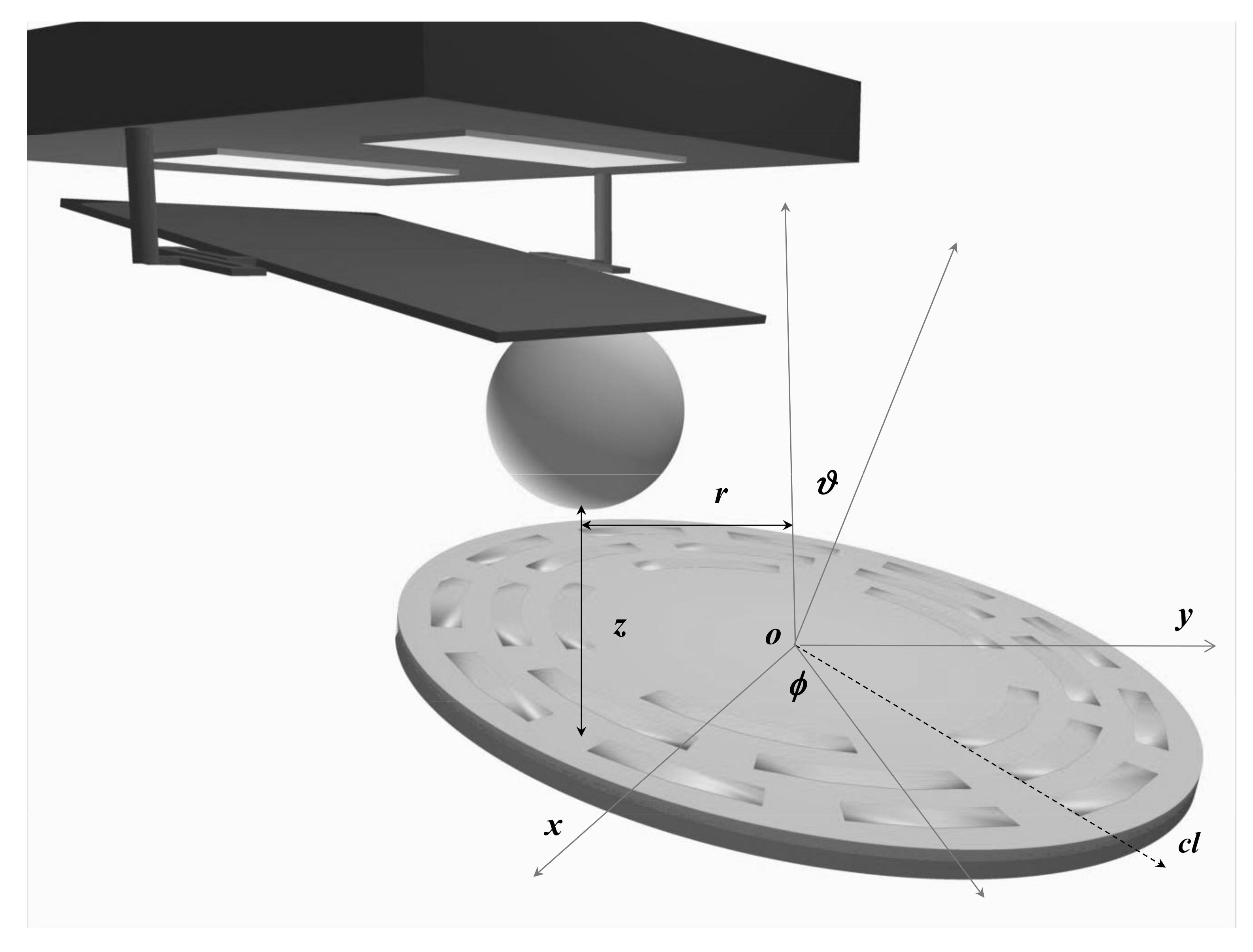
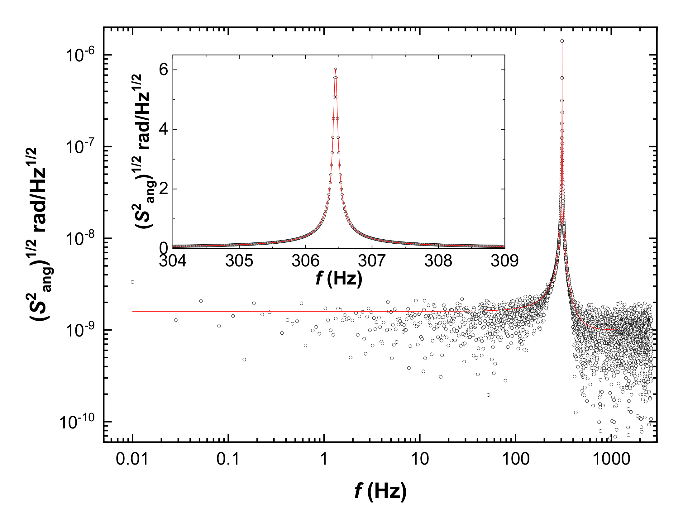
The radius of the sapphire sphere covered with Cr and Au ($d_{\mathrm{Au}}^{\mathrm{sphere}}\approx 250$ nm) is determined by scanning electron microscopy to be $R=$(149.7 ± 0.2) $\mathsf{\mu }$m. The deposited Au on the sapphire sphere is characterized by atomic force microscopy (AFM) images, and the rms roughness is found to be $t_{\mathrm{rms}}=0.27$ nm. This was obtained by doing 6 non-overlapping $5\times 5\mathsf{\mu }$m${}^2$ (1024 × 1024 pixels${}^2$) scans over the coated sphere near the position of the sphere closest to the sample.

As aforementioned, trenches in the rotating sample are fabricated by DRIE followed by the deposition of $d_{\mathrm{Cr}}\approx 10$ nm thick layer of Cr followed by $d_{\mathrm{Au}}^{\mathrm{sample}}\approx 150$ nm on a 1 inch diameter $100\mathsf{\mu }$m thick [100] oriented Si wafer. To make the trenches $\approx 3\mathsf{\mu }$m thick photoresist is spun-coated on the Si wafer, and using conventional photolithographic approach the photoresist is removed from the pattern with the concentric sectors (where the trenches would be defined). Afterwards, C${}_4$F${}_8$ deposition provides the fluorocarbon coating of all surfaces, and SF${}_6$ provides the fluorine for isotropic etching. The fluorine does not etch the fluorocarbon coating, and sputters it by mechanical etching at the bottom, consequently etching the exposed Si. The cycle forms nanoscallops on the lateral surface, and it is repeated until the desired depth of the trenches is obtained. During the process each cycle was tuned to remove about 150 nm of Si. When the desired depth is achieved a final plasma etching step is used to remove the residual C${}_4$F${}_8$. The average position of the formed wall is found to be nearly vertical (the measured angle as determined by SEM inspection in similar structures is observed to be larger than 89.5${}^{\mathrm{\circ }}$). Exposed Au surfaces are characterized by white light interferometry (WLI) and atomic force microscopy (AFM). Both techniques show an optical quality Au film deposited on top of the Si wafer. The 1024 × 1024 pixel${}^2$ AFM images obtained over different $10\times 10\mathsf{\mu }{\mathrm{m}}^2$ regions show position-independent ≈ 10 nm peak-to-peak roughness with the rms deviations from the mean level of less than 0.4 nm. It was not possible, however, to determine the quality and overall thickness of the Cr/Au layers deposited on the sidewalls and bottom of the trenches. The disk is mounted on the air bearing spindle. It is optically verified that the center of the disk and the axis of rotation of the spindle coincided to better than $\Delta r\approx 5\mathsf{\mu }$m by measuring the gap between the edge of the disk and the edge of the indentation where the disk sits. The flatness and alignment of the sample are checked in-situ using a fiber interferometer (response time 10 ms). The surface of the sample is perpendicular to the axis of rotation to better than $z_{\mathrm{o}}$ = 20 nm at ${}^{300}r$ when rotating the disk at $\omega =2\pi$ rad/s.

2.2. Oscillators

The MTOs are similar to the ones used in previous experiments [9,10,11,12,18,25,33]. Differently from some of the previous measurements and as schematically shown in Figure 1 the metal coated spheres are glued close to the edge of the plate of the oscillator. Gluing the Au-coated spheres at a distance $b=(239\pm 4)\mathsf{\mu }$m from the axis of rotation reduced the MTO’s natural frequency of oscillation from $f_{\mathrm{o}}\simeq 700$ Hz to $f_{\mathrm{r}}=(306.45\pm 0.02)$ Hz. The quality factor was reduced from $\approx 9000$ to $Q=4850$.

The power spectral density $S_{\alpha }^2(f)$ of the oscillator is shown in Figure 2. For a torsional simple harmonic damped oscillator driven by thermal fluctuations the angular response in the torsional angle $\alpha$ is [36]

$$S_{\alpha }^2(f)=\frac{2k_{\mathrm{B}}T}{\pi \kappa Q{f}_{\mathrm{r}}}\frac{f_{\mathrm{r}}^4}{{(f_{\mathrm{r}}^2-f^2)}^2+f^2{f}_{\mathrm{r}}^2/Q^2}+S_{\mathrm{elec}}^2,$$

(2)

where an independently determined flat detection noise term $S_{\mathrm{elec}}^2$ associated with the electronic measurement setup [18] has been added. In (2), $k_{\mathrm{B}}$ is Boltzmann’s constant, T the temperature at which the experiment is performed, ${\kappa }_{\mathrm{MTO}}$ is the MTO’s torsional constant. Doing the measurement at resonance, where the $1/f$ term and the detection noise are negligible, it is found that the minimum detectable force (per Hz${}^{1/2}$) is

$$\frac{1}{b}\sqrt{\frac{2{\kappa }_{\mathrm{MTO}}{k}_{\mathrm{B}}T}{\pi Q{f}_{\mathrm{r}}}}\sim 6\frac{\mathrm{fN}}{\sqrt{\mathrm{Hz}}}.$$

(3)

With the achieved temperature control, the drift in the resonant $f_{\mathrm{r}}$ is less than 0.3 mHz/hr under operating conditions.

2.3. Electrostatic Calibration and Separation Determination

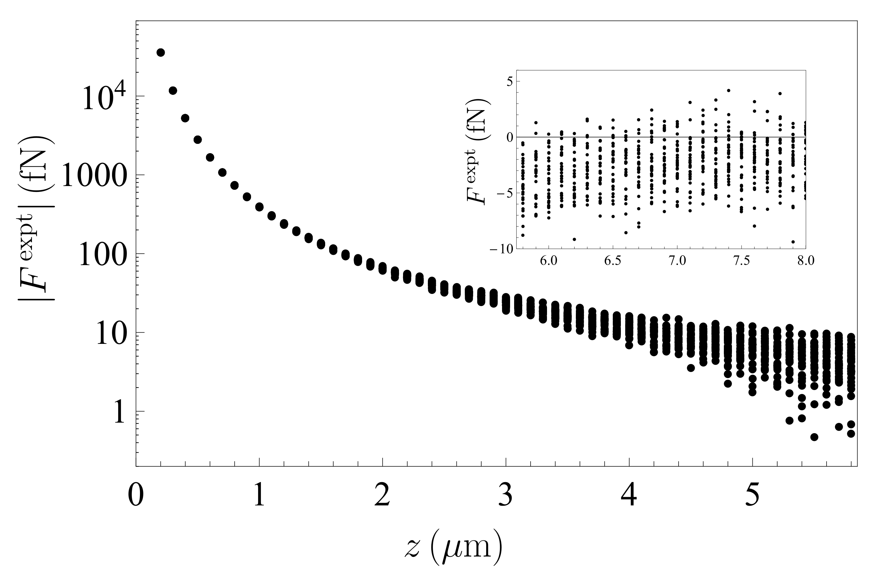
The system’s calibration is performed similarly to what was done in [37]. An optical fiber was rigidly attached to the MTO-sphere assembly, and a two-color interferometer was used to measure the distance between the end of the fiber and a stationary platform. Simultaneously $f_{\mathrm{r}}$ and the angular deviation of the MTO were recorded as the sphere is moved closer to the sample. From the change in $f_{\mathrm{r}}(z)$ the gradient of the interaction between the sphere and the plate can be obtained when a potential difference is applied between them. Comparing the separation dependence of the gradient of the interaction with that of the known sphere-plate electrostatic interaction

$$\begin{array}{ccc}& & F_e(z,V)=-2\pi {\epsilon }_0{(V-V_{\mathrm{o}})}^2\sum _{n=0}^{\infty }\frac{coth(u)-ncoth(nu)}{sinh(nu)}\hfill \\ & & \phantom{F_e(z,V)}=-2\pi {\epsilon }_0{(V-V_{\mathrm{o}})}^2\sum _{m=0}^7{A}_m{q}^{m-1},\hfill \end{array}$$

(4)

the parameters of the system are obtained. In (4), ${\epsilon }_0$ is the permittivity of free space (in SI units), V is a potential applied to the sample (the sphere-oscillator assembly is always kept grounded) and $V_{\mathrm{o}}$ is a residual potential difference between the plate and the sphere, $u=1+z/R$, $A_m$ are fitting coefficients, and $q=z/R$. While the full expression is exact, the series is slowly convergent, and it is easier to use the shown approximation developed in [38]. Using this approach, ${\kappa }_{\mathrm{MTO}}=(1.07\pm 0.01)\times {10}^{-9}$ Nm/rad is obtained, with $V_{\mathrm{o}}$ of the order of a few mV. For all configurations used, $V_{\mathrm{o}}$ was checked to be position and time independent. As customary in these experiments, the differential measurements are performed with $V=V_{\mathrm{o}}$ to minimize the electrostatic contribution.

In order to simplify the data acquisition and control of the system, during the experiment the two-color interferometer is used such that it controls the separation between the sphere-MTO assembly and a fixed platform, yielding a measurement of the distance $z_{\mathrm{meas}}$ between the end of the fiber and the fixed platform. In order to find the separation z between the sphere and the top of the rotating disc

$$z=z_{\mathrm{meas}}-D_1-D_2-b\alpha ,$$

(5)

the quantity $D_1+D_2$ is obtained from the electrostatic calibration. In (5), $D_1$ is the fixed distance between the end of the fiber and the vertex of the sphere when the system is relaxed, and $D_2$ is the distance between the fixed platform and the top of the rotating sample. At each measurement position the torsional angle $\alpha$ is measured with the sphere on top of the Au region, away from the regions with trenches (i.e., no signal is expected at $f_{}$ in this situation) and the value of $\alpha$ (which is always smaller than ${10}^{-5}$ rad) is determined from the difference in capacitance between the MTO’s plate and the two underlying electrodes. Hence, from the measured value $z_{\mathrm{meas}}$, the fitted $D_1+D_2$, the optically determined b and the capacitively determined $\alpha$, the separation z is found.

2.4. Results

Extraction of the data is done assuming the interaction between the sphere and the trenches follows a Heaviside function as the sample rotates under the sphere. Under this condition, the force values reported are $\pi /4$ times the measured value at the corresponding harmonic. At each point the force value was determined from the first harmonic. The force measurements were repeated 30 times in the separation region from 200 nm to $8\mathsf{\mu }$m with a step of 100 nm. Each repetition was measured with an integration time of 100 s. In Figure 3 the obtained results (30 force magnitudes at each separation) are shown in logarithmic scale over the region from 0.2 to $5.8\mathsf{\mu }$m. In the inset, the measured forces over the region from 5.8 to $8\mathsf{\mu }$m are presented in linear scale. The form of the distribution law and the random errors of the measurement results are considered in Section 6.1.

3. Systematic Errors and Edge Effects

In this section, we consider different contributions to the total systematic error in measuring the Casimir force by means of a micromechanical torsional oscillator. Taking into account that in our case the disc in Figure 1 is not flat but contains deep, concentrically situated trenches, we also investigate the size of possible errors in the measured force which could arise from edge effects.

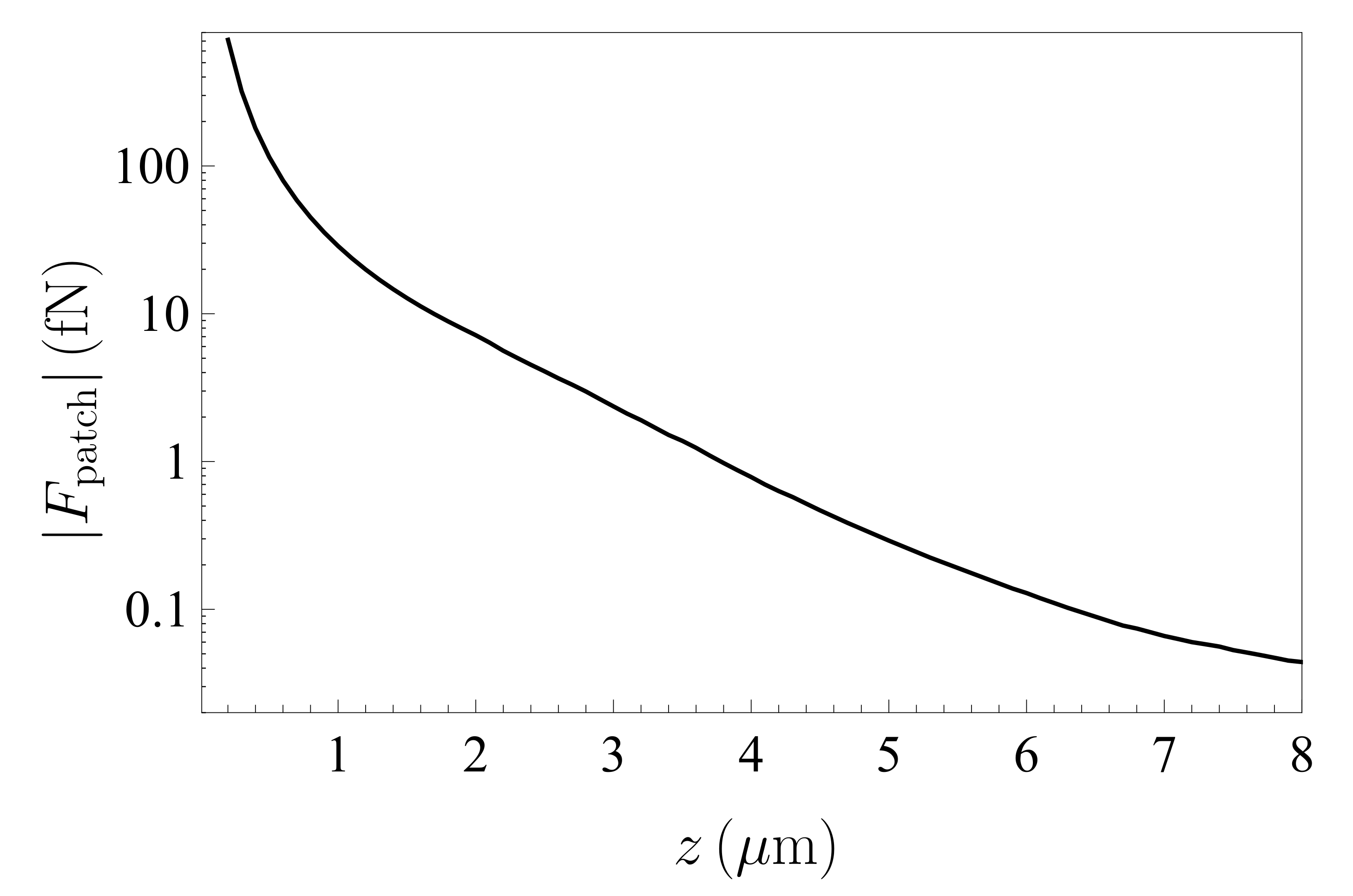
3.1. Contributions to the Systematic Error

The success of the experiment resides in having a controlled metrological environment for the interaction and separation (as described in Section 2.3) but since also a lock-in amplifier technique is used, it is imperative to preserve a tight time and frequency synchronization. Time synchronization is achieved by focusing a diffraction limited laser on the rotating sample at a distance $r\approx 9$ mm from its rotational axis. The sample itself has a region where no Au is deposited located in $r\in [8.5,9.5]$ mm subtending an angle of $2\times {10}^{-4}$ rad. The leading edge of this sector is along the cl-line. As the sample rotates, the change in reflection of the focused laser is used as a trigger for all timed events. It has been verified that this trigger lags by ${\tau }_{\mathrm{lag}}={10}^{-6}/f$. The rotation frequency is obtained by finding the maximum of the thermally induced peak shown in Figure 2 with an accumulation time of 100 s. The required multiple of this signal is synthesized and fed to the air bearing spindle.

In general, with the sphere placed at ${}^{300}{r}_{\mathrm{i}}+75\mathsf{\mu }$m, the air bearing spindle was rotated at $\omega =2\pi f_{\mathrm{r}}/300$. In this manner, a force arising from the difference in the Casimir force between the metal coated sphere and the layered structure manifests itself at $f_{\mathrm{r}}$ even though there are no parts moving at $f_r$. Using lock-in detection at $f_{\mathrm{r}}$ signals which are small but could show in conventional experiments are removed by the averaging provided by the rotating sample and the high-Q of the MTO. While this approach is employed to obtain the interaction, the large range of separations used and the consequent large change in the strength of the interaction presents a drawback: at the short end of the range in z the relatively large force difference between the situations when the sphere is on top of the ridges or trenches would cause the oscillator to behave non-linearly or break. To prevent this, the measurements at small z are detuned from $f_{\mathrm{r}}$. Since now the system is at a steep part of the resonance curve, the errors in frequency stability are amplified when compared to the corresponding errors at large z when the measurements can be done at resonance.

It is known from previous studies [18,25] that the air bearing spindle has a revolution impulsive kick on the order of $\vartheta \sim {10}^{-7}$ rad. Fortunately in the measurements performed in this study this does not affect the measurement. The system was positioned such that when the impulsive kick happens, the sphere is located over a trench and there is no effect on the measurement. In all measurements it is observed that when $z>20\mathsf{\mu }$m the expression shown in (3) is verified: As the integration time $\tau$ increases, the detectable force decreases as 5.8 fN/$\sqrt{\mathrm{Hz}\tau }$.

Contributions to the systematic errors of measurements are summarized in

Table 1. Systematic errors in the separation and determination of the measured force. The errors in b ($4\mathsf{\mu }$m) and $\alpha$ (0.8 nrad) do not contribute to the overall error of separation. The listed error in $D_1+D_2$ is obtained from the electrostatic calibration. The error reported in $z_{\mathrm{meas}}$ is larger than the local measured error of 0.2 nm due to the fact that the rotating sample has measured height difference of ≈1.2 nm. This is not adjusted during rotation. The force measurement error varies from 85 fN at the shortest separation to 0.5 fN at $z⩾1$ μm. All errors are at the 95% confidence level.

	${\mathit{D}}_1+{\mathit{D}}_2$ [nm]	${\mathit{z}}_{\mathbf{meas}}$ [nm]	Flatness of wafer [nm]
Separation	0.6	0.2	1.2
	Detection [fN]	Calibration [fN]	Measurement [fN]
Force	0.6	0.2	[85, 0.5]

.

There is one more uncertainty in an interpretation of the measured force signal as the Casimir force. It is connected with the contribution of patch potentials. The sample was characterized by Kelvin probe microscopy, and the potential distribution was found to be similar to the one in [39] with $V_{\mathrm{rms}}\approx 12$mV and average size of patches $\overline{l}\approx 250$nm. At the smallest separation $z_1=200$nm, the attractive force due to the presence of patches can be estimated as $|F_{\mathrm{patch}}|\approx 0.7$pN (see Figure 4 of [40]), that is, of about 2% of the measured Casimir force. Using the asymptotic expression [40]

$$F_{\mathrm{patch}}(z)=-\pi \zeta (3)R\frac{{\epsilon }_0{V}_{\mathrm{rms}}^2{\overline{l}}^2}{2z^3},$$

(6)

which is well applicable at $z>7\mathsf{\mu }$m, the estimated magnitude of the force originating from the surface patches is shown in Figure 4 over the entire measurement range.

3.2. Investigation of Edge Effects

In what follows, we analyze the edge effects, that is, possible deviations of a signal shape from the Heaviside function during rotation. In order to do this analysis, 21 harmonics of the measured signal were determined at four separations $z=$ 200, 500, 1000, and 5000 nm. At these separations all measured force values are negative (see Figure 3). Below we consider the force magnitudes. To measure the m-th harmonic of the signal, the sample was rotated at an angular frequency ${\omega }_m=2\pi f_{\mathrm{r}}/(m{n}_{\mathrm{tr}})$ (recall that $n_{\mathrm{tr}}$ is the number of alternating Au trenches). Furthermore, the even and odd contributions to the signal are selected by setting the phase of the lock-in detection to 0 when the sphere crosses the line cl (see Figure 1).

The general properties of the Fourier series of the signal are what follows next. Let $\widehat{\varphi }$ be an angle variable, defined such that $\widehat{\varphi }$ changes by $2\pi$ as one traverses a Au sector and a trench. Up to random patch effects and other sources of noise, the signal $F(\widehat{\varphi })$ is then $2\pi$ periodic:

$$F(\widehat{\varphi }+2\pi )=F(\widehat{\varphi }).$$

(7)

If the origin of the angles is taken to be in the center of a Au sector, the force signal is also expected to be symmetric with respect to an inversion of $\widehat{\varphi }$:

$$F(-\widehat{\varphi })=F(\widehat{\varphi }).$$

(8)

It follows from (7) and (8) that the Fourier expansion of the signal contains only cosines and, thus, is of the form:

$$F(\widehat{\varphi })=\frac{a_0}{2}+\sum _{m=1}^{\infty }{a}_{m}cos(m\widehat{\varphi }).$$

(9)

To proceed, we make the assumption that the signal can be represented as a sum of the step function $F\chi (\widehat{\varphi })$ plus an edge correction $f(\widehat{\varphi })$:

$$F(\widehat{\varphi })=|F|\chi (\widehat{\varphi })+f(\widehat{\varphi }),$$

(10)

where F is the force between an Au sphere and a homogeneous Au plate, and $\chi (\widehat{\varphi })$ is the $2\pi$ periodically continued step function of the interval $[-\pi ,\pi ]$, which is equal to unity for $-\pi /2⩽\widehat{\varphi }⩽\pi /2$ and zero elsewhere. The correction $f(\widehat{\varphi })$ represents the effect of the edges, which includes both edge-corrections to the Casimir force as well as stray electrostatic forces arising from charges localized along the edges. We assume that $f(\widehat{\varphi })$ is localized in a narrow region of angular width $ϵ$ across the edges of the Au sectors. According to (10) we decompose the Fourier coefficients $a_m$ as:

$$a_m=a_m^{(\mathrm{step})}+\delta a_m,$$

(11)

where $a_m^{(\mathrm{step})}$ is the contribution of the step function and $\delta a_m$ is the edge correction. By a straightforward computation one finds that the coefficients $a_m^{(\mathrm{step})}$ are zero for even m, while for odd m one finds:

$$a_{2p-1}^{(\mathrm{step})}=-{(-1)}^p\frac{2|F|}{\pi (2p-1)},p=1,2,\dots$$

(12)

On the other hand, for the corrections $\delta a_m$ one finds:

$$\delta a_m=\frac{2}{\pi }{\int }_{\pi /2-ϵ}^{\pi /2+ϵ}d\widehat{\varphi }f(\widehat{\varphi })cos(m\widehat{\varphi })=\frac{2}{\pi }{\int }_{-ϵ}^{ϵ}dxf\left(\frac{\pi }{2}+x\right)cos\left[m\left(\frac{\pi }{2}+x\right)\right].$$

(13)

Since the width $ϵ$ of the edge region is small, for m not too large it is possible to take the Taylor expansion of the cosines in power of x. By Taylor expanding the cosines around $\widehat{\varphi }=\pi /2$ up to order $x^2$ included, for even $m=2p$, $p=1,2,\dots$ one finds:

$$\delta a_{2p}=\frac{2}{\pi }{(-1)}^p\left[f^{(0)}-2p^2{f}^{(2)}\right],$$

(14)

while for odd $m=2p-1$, $p=1,2,\dots$ one finds:

$$\delta a_{2p-1}=\frac{2}{\pi }{(-1)}^p(2p-1)f^{(1)},$$

(15)

where $f^{(q)}$ is the q-th moment of the edge correction:

$$f^{(q)}={\int }_{-ϵ}^{ϵ}dx{x}^{q}f\left(\frac{\pi }{2}+x\right).$$

(16)

Combining (12)–(15), we find that the leading Fourier coefficients in (9) are those with odd $m=2p-1$:

$$a_{2p-1}=-\frac{2}{\pi }{(-1)}^p\left[\frac{|F|}{2p-1}-(2p-1)f^{(1)}\right],$$

(17)

while for even $m=2p$ the Fourier coefficients coincide with the edge correction:

$$a_{2p}=\frac{2}{\pi }{(-1)}^p\left[f^{(0)}-2p^2{f}^{(2)}\right].$$

(18)

In the experiment, angles are measured starting from the edge of a Au sector. Thus we define the shifted angle variable $\overline{\varphi }$ such that $\widehat{\varphi }=\overline{\varphi }-\pi /2$. When re-expressed in terms of $\overline{\varphi }$, the Fourier expansion in (9) takes the form:

$$F(\overline{\varphi })=\frac{a_0}{2}+\sum _{p=1}^{\infty }{(-1)}^p\left\{a_{2p}cos(2p\overline{\varphi })-a_{2p-1}sin\left[(2p-1)\overline{\varphi }\right]\right\}.$$

(19)

In reality, the origin of the angles cannot exactly coincide with the edge of Au sector, and we should allow for a possible small phase $\delta$. From the sample design and the time synchronization procedure, $\delta$ is expected to be of order:

$$|\delta |\sim {10}^{-4}\mathrm{rad}.$$

(20)

We define the final angle variable $\varphi$ such that $\overline{\varphi }=\varphi -\delta$. When the series in (19) is re-expressed in terms of $\varphi$, and only leading terms in the small phase $\delta$ are retained, one obtains:

$$\begin{array}{ccc}& & F(\varphi )=\frac{a_0}{2}+\frac{2}{\pi }\sum _{p=1}^{\infty }\left\{\phantom{\left[\frac{|F|}{2p-1}-(2p-1)f^{(1)}\right]}\left[f^{(0)}-2p^2{f}^{(2)}\right]cos(2p\varphi )-|F|\delta cos\left[(2p-1)\varphi \right]\right.\hfill \\ & & \left.+\left[\frac{|F|}{2p-1}-(2p-1)f^{(1)}\right]sin\left[(2p-1)\varphi \right]+f^{(0)}2p\delta sin(2p\varphi )\right\}.\hfill \end{array}$$

(21)

We remind that the expressions of the Fourier coefficients in the above equation are valid for harmonics such that $pϵ\ll 1$ and $p\delta \ll 1$. We assume that both conditions are satisfied for the measured harmonics. The final Fourier expansion (21) is of the form:

$$F(\varphi )=\frac{a_0}{2}+\sum _{m=1}^{\infty }\left[b_{m}sin(m\varphi )+c_{m}cos(m\varphi )\right].$$

(22)

Its general features are as follows:

(1) The dominant terms are sines with odd m and the coefficients:

$$b_{2p-1}=\frac{2}{\pi }\left[\frac{|F|}{2p-1}-(2p-1)f^{(1)}\right].$$

(23)

(2) The coefficients $b_{2p}$ of sines with even m are proportional to the phase shift $\delta$ and to the first moment $f^{(0)}$ of the edge correction. Moreover, they are linear in the Fourier index $m=2p$:

$$b_{2p}=\frac{2}{\pi }{f}^{(0)}2p\delta .$$

(24)

(3) The coefficients $c_{2p}$ of the cosines with even m depend on the moments $f^{(0)}$ and $f^{(2)}$ of the edge correction, and have a quadratic dependence on the index $m=2p$:

$$c_{2p}=\frac{2}{\pi }\left[f^{(0)}-2p^2{f}^{(2)}\right].$$

(25)

Finally, the coefficients of the cosines with odd m are proportional to the phase shift $\delta$ and are independent of the order $m=2p-1$:

$$c_{2p-1}=-\frac{2}{\pi }|F|\delta .$$

(26)

Based on the above equations, one can predict that the Fourier coefficients satisfy the following hierarchy:

$$b_{2p-1}\gg c_{2p}\gg b_{2p}\sim c_{2p-1},$$

(27)

which was verified to be true.

We used (21) to analyze the 21 measured harmonics for the nominal sphere-plate separations $z=200$, 500, 1000, 5000 nm. As an example, below we present the results obtained at $z=200$nm. In Figure 5 we show the data for the sines with odd m for $z=200$ nm, and the fit by a curve of the form $b_m=u_1/m+u_{2}m$. The agreement is excellent as it can be seen from Figure 6 where we show the differences between the data and the fitting curve. Since for each measured harmonic only one measurement was made, it was in principle impossible to determine their error. To circumvent this problem, we assumed that the error for the 21 harmonics is the same, and thus we estimated the common standard deviation $\sigma$ of the odd coefficients $b_{2p-1}$ by the formula:

$${\sigma }_{200\mathrm{nm}}^2=\frac{1}{9}\sum _{p=1}^{11}{\left[b_{2p-1}-\frac{{\overline{u}}_1}{2p-1}-{\overline{u}}_2(2p-1)\right]}^2,$$

(28)

where ${\overline{u}}_1$ and ${\overline{u}}_2$ are best fit values. The sum over p is divided by 9 because there are 11 Fourier coefficients and two free parameters ($u_1$ and $u_2$). We obtained:

$${\sigma }_{200\mathrm{nm}}=0.6\mathrm{fN}.$$

(29)

The values of $\sigma$ that were obtained for the other Fourier coefficients $b_{2p}$, $c_{2p-1}$ and $c_{2p}$ have a similar magnitude, for all the four considered separations. For example, from $b_{2p-1}$ we find:

$${\sigma }_{500\mathrm{nm}}=0.5\mathrm{fN},{\sigma }_{1000\mathrm{nm}}=0.4\mathrm{fN},{\sigma }_{5000\mathrm{nm}}=0.6\mathrm{fN}.$$

(30)

Using the estimates (29) and (30) of the standard deviations, we were able to determine the forces and edge corrections at the desirable confidence level.

The best fit of the Fourier coefficients $b_m$, with odd m provides the following estimate of the force at $z=200$nm:

$$F^{\mathrm{expt}}=(-3.5675\pm 0.0003)\times {10}^{-11}\mathrm{N}$$

(31)

and of the edge correction

$$f^{(1)}=(6.01\pm 0.06)\times {10}^{-15}\mathrm{N},$$

(32)

where both errors correspond to the 99% confidence level.

Next we consider the data for cosines with even m. These are shown in Figure 7. The solid line is a fit with a quadratic curve $c_m=v_0+v_2{m}^2$, as per (25). The agreement is excellent as it can be seen from Figure 8 where we show the differences between the data and the fitting curve.

From the fit we obtain:

$$f^{(0)}=(6.013\pm 0.010)\times {10}^{-13}\mathrm{N},f^{(2)}=(1.03\pm 0.10)\times {10}^{-16}\mathrm{N},$$

(33)

where both errors correspond to the 99% confidence level. Equations (32) and (33) show that there indeed is an edge effect, but fortunately it is negligibly small.

Now we turn our attention to the data for cosines with odd m, which, according to (26), should be independent of the Fourier index $m=2p-1$. The respective data are shown in Figure 9 (left). As is seen in this figure, the data are really almost independent of the Fourier index. The observed deviations have the character of statistical fluctuations. The fit gives:

$$\delta =-2\times {10}^{-4}\mathrm{rad},$$

(34)

in accordance with the expected magnitude of $\delta$ in (20).

We finally consider the Fourier coefficients for sines with even m. The data are shown in Figure 9 (right), together with a plot of the linear dependence (24). The line drawn in Figure 9 (right) uses the values of $\delta$ and $f^{(0)}$ determined previously. The fairly good agreement between (24) and the data provides a further validation of the theoretical model of the signal (21).

The overall analysis of the signal rules out any important influence of edge effects and justifies modelling the interaction between the sphere and the sample by a Heaviside function.

4. Exact Evaluation of the Casimir Force in Sphere-Plate Geometry Using the Scattering Formula

In this section, we calculate the Casimir force between an Au sphere and an Au plate on the basis of first principles of quantum electrodynamics. This is especially important for subsequent comparison between experiment and theory at separations of a few micrometers where the approximate methods like the proximity force approximation (PFA) become less exact. Below we review the theoretical basis for the numerical determination of the Casimir force using electromagnetic plane waves which has been employed to determine the exact results presented in this paper. We aim at a coherent presentation of results presented in different places in the literature [27,28,29].

Within the scattering formalism, the Casimir free energy $\mathcal{F}$ between a sphere and a plane at a surface-to-surface distance z can be expressed through [41,42,43,44,45]

$$\mathcal{F}=k_{B}T\sum _{l=0}^{\infty }{}^{\prime }logdet[1-\mathcal{M}(i{\xi }_l)],$$

(35)

where the primed sum indicates that the $l=0$ term is weighted by a factor of $1/2$, the Matsubara frequencies are given by ${\xi }_l=2\pi k_{B}Tl/\hslash$ and the round-trip operator is defined as

$$\mathcal{M}={\mathcal{T}}_{\mathrm{PS}}{\mathcal{R}}_{\mathrm{S}}{\mathcal{T}}_{\mathrm{SP}}{\mathcal{R}}_{\mathrm{P}}.$$

(36)

Here, ${\mathcal{R}}_{\mathrm{P}}$ and ${\mathcal{R}}_{\mathrm{S}}$ denote the reflection operator at the plane and sphere, respectively, while ${\mathcal{T}}_{\mathrm{PS}}$ stands for the translation operator from the sphere center to the surface of the plane and vice versa for ${\mathcal{T}}_{\mathrm{SP}}$.

The scattering formula for the Casimir force F can be found from (35) by taking the negative derivative with respect to the surface-to-surface separation z. Application of Jacobi’s formula then yields

$$F=-\frac{\partial \mathcal{F}}{\partial z}=k_{B}T\sum _{l=0}^{\infty }{}^{\prime }\mathrm{tr}\left(\frac{{\partial }_z\mathcal{M}}{1-\mathcal{M}}\right).$$

(37)

The round-trip operator (36) and its constituents act on electromagnetic modes which are solutions of the Helmholtz equations. Through the determinant in (35) and the trace in (37) it is evident that one is free to choose a basis in which those electromagnetic modes are expanded. Usually, spherical multipoles are employed [46,47,48,49]. Recently, it was shown that a basis consisting of plane waves shows far better convergence rates [29]. Here, we thus employ the approach based on plane waves. In the following, we review the plane-wave numerical approach from [29] and give the relevant ingredients for the sphere-plate problem.

4.1. Plane-Wave Representation

Within the angular spectrum decomposition, we define the plane-wave basis by the set $\left\{|\mathbf{k},\mathsf{{\rm Y}},\varrho \rangle \right\}$ with the component of the wave vector transverse to the z-axis $\mathbf{k}$, the propagation direction with respect to the z-axis $\mathsf{{\rm Y}}=\pm$ and $\varrho =\mathrm{TE},\mathrm{TM}$ denoting transverse electric and transverse magnetic polarizations, respectively. Even though the plane-wave basis elements also depend on the imaginary frequency $\xi$, we suppress it as $\xi$ is conserved throughout a round-trip.

When expanding in the plane-wave basis, each operator $\mathcal{O}$ appearing in (36) becomes an integral operator defined through its corresponding scalar kernel function $f_{\mathcal{O}}$. These kernel functions correspond to the plane-wave matrix elements of the respective operators. For instance, the action of the round-trip operator on a plane-wave basis element can be written as

$$\mathcal{M}|\mathbf{k},-,\varrho \rangle =\sum _{{\varrho }^{\prime }}\int \frac{d^2{k}^{\prime }}{{(2\pi )}^2}{f}_{\mathcal{M}}({\mathbf{k}}^{\prime },{\varrho }^{\prime };\mathbf{k},\varrho )|{\mathbf{k}}^{\prime },-,{\varrho }^{\prime }\rangle$$

(38)

in terms of the kernel function of the round-trip operator $f_{\mathcal{M}}$.

The translation operators and the reflection operator on the plane are diagonal in the plane-wave basis. Their corresponding kernel functions read

$$\begin{array}{cc}\hfill f_{{\mathcal{T}}_{\mathrm{PS}}}({\mathbf{k}}^{\prime },{\varrho }^{\prime };\mathbf{k},\varrho )& =f_{{\mathcal{T}}_{\mathrm{SP}}}({\mathbf{k}}^{\prime },{\varrho }^{\prime };\mathbf{k},\varrho )={(2\pi )}^2{e}^{-\kappa (z+R)}{\delta }_{\varrho ,{\varrho }^{\prime }}\delta (\mathbf{k}-{\mathbf{k}}^{\prime }),\hfill \\ \hfill f_{{\mathcal{R}}_{\mathrm{P}}}({\mathbf{k}}^{\prime },{\varrho }^{\prime };\mathbf{k},\varrho )& ={(2\pi )}^2{r}_{\varrho }{\delta }_{\varrho ,{\varrho }^{\prime }}\delta (\mathbf{k}-{\mathbf{k}}^{\prime })\hfill \end{array}$$

(39)

with

$$\kappa =\sqrt{K^2+{\mathbf{k}}^2},$$

(40)

where the imaginary vacuum wave number $K=\xi /c$ and the Fresnel reflection coefficients are

$$\begin{array}{cc}\hfill r_{\mathrm{TE}}& =\frac{\kappa -\sqrt{(\epsilon -1)K^2+{\kappa }^2}}{\kappa +\sqrt{(\epsilon -1)K^2+{\kappa }^2}},\hfill \\ \hfill r_{\mathrm{TM}}& =\frac{\epsilon \kappa -\sqrt{(\epsilon -1)K^2+{\kappa }^2}}{\epsilon \kappa +\sqrt{(\epsilon -1)K^2+{\kappa }^2}}.\hfill \end{array}$$

(41)

The Fresnel reflection coefficients (41) depend explicitly on the dielectric permittivity $\epsilon =\epsilon (i\xi )$.

The reflection on the sphere is only diagonal in the polarization basis defined with respect to the scattering plane. In the TE-TM polarization basis taken with respect to the plate surface, the reflection operator is, however, not diagonal. Within the sphere-plate geometry, the kernel function of the round-trip operator is thus proportional to the kernel function of the reflection operator on the sphere:

$$f_{\mathcal{M}}({\mathbf{k}}^{\prime },{\varrho }^{\prime };\mathbf{k},\varrho )=r_{\varrho }{e}^{-(\kappa +{\kappa }^{\prime })(z+R)}{f}_{{\mathcal{R}}_{\mathrm{S}}}({\mathbf{k}}^{\prime },{\varrho }^{\prime };\mathbf{k},\varrho ),$$

(42)

where [27,28]

$$\begin{array}{cc}\hfill f_{{\mathcal{R}}_{\mathrm{S}}}({\mathbf{k}}^{\prime },\mathrm{TM};\mathbf{k},\mathrm{TM})& =\frac{2\pi }{K{\kappa }^{\prime }}(A{S}_2+B{S}_1),\hfill \\ \hfill f_{{\mathcal{R}}_{\mathrm{S}}}({\mathbf{k}}^{\prime },\mathrm{TE};\mathbf{k},\mathrm{TE})& =\frac{2\pi }{K{\kappa }^{\prime }}(A{S}_1+B{S}_2),\hfill \\ \hfill f_{{\mathcal{R}}_{\mathrm{S}}}({\mathbf{k}}^{\prime },\mathrm{TM};\mathbf{k},\mathrm{TE})& =-\frac{2\pi }{K{\kappa }^{\prime }}(C{S}_1+D{S}_2),\hfill \\ \hfill f_{{\mathcal{R}}_{\mathrm{S}}}({\mathbf{k}}^{\prime },\mathrm{TE};\mathbf{k},\mathrm{TM})& =\frac{2\pi }{K{\kappa }^{\prime }}(C{S}_2+D{S}_1),\hfill \end{array}$$

(43)

with ${\kappa }^{\prime }$ defined as in (40) and the plane-wave scattering amplitudes [50]

$$\begin{array}{cc}\hfill S_1& =\sum _{\ell =1}^{\infty }\frac{2\ell +1}{\ell (\ell +1)}\left[a_{\ell }(iKR){\pi }_{\ell }(cos\Theta )+b_{\ell }(iKR){\tau }_{\ell }(cos\Theta )\right],\hfill \\ \hfill S_2& =\sum _{\ell =1}^{\infty }\frac{2\ell +1}{\ell (\ell +1)}\left[a_{\ell }(iKR){\tau }_{\ell }(cos\Theta )+b_{\ell }(iKR){\pi }_{\ell }(cos\Theta )\right].\hfill \end{array}$$

(44)

These plane-wave scattering amplitudes depend on the material properties of the sphere through the Mie coefficients [50]

$$\begin{array}{cc}\hfill a_{\ell }(ix)& ={(-1)}^{\ell }\frac{\pi }{2}\frac{n^2{s}_{\ell }^{(a)}-s_{\ell }^{(b)}}{n^2{s}_{\ell }^{(c)}+s_{\ell }^{(d)}},\hfill \\ \hfill b_{\ell }(ix)& ={(-1)}^{\ell +1}\frac{\pi }{2}\frac{s_{\ell }^{(b)}-s_{\ell }^{(a)}}{s_{\ell }^{(c)}+s_{\ell }^{(d)}}\hfill \end{array}$$

(45)

for electric and magnetic polarizations, respectively, where

$$\begin{array}{cc}\hfill s_{\ell }^{(a)}& =I_{\ell +\frac{1}{2}}(nx)\left[x{I}_{\ell -\frac{1}{2}}(x)-\ell I_{\ell +\frac{1}{2}}(x)\right],\hfill \\ \hfill s_{\ell }^{(b)}& =I_{\ell +\frac{1}{2}}(x)\left[nx{I}_{\ell -\frac{1}{2}}(nx)-\ell I_{\ell +\frac{1}{2}}(nx)\right],\hfill \\ \hfill s_{\ell }^{(c)}& =I_{\ell +\frac{1}{2}}(nx)\left[x{K}_{\ell -\frac{1}{2}}(x)+\ell K_{\ell +\frac{1}{2}}(x)\right],\hfill \\ \hfill s_{\ell }^{(d)}& =K_{\ell +\frac{1}{2}}(x)\left[nx{I}_{\ell -\frac{1}{2}}(nx)-\ell I_{\ell +\frac{1}{2}}(nx)\right]\hfill \end{array}$$

(46)

with $I_{\ell }$ and $K_{\ell }$ being the modified Bessel functions of first and second kind [51] and $n=n(i\xi )=\sqrt{\epsilon (i\xi )}$ the refractive index of the sphere. The angular functions ${\pi }_{\ell }$ and ${\tau }_{\ell }$ appearing in (44) are defined as [50]

$$\begin{array}{cc}\hfill {\pi }_{\ell }(z)& =P_{\ell }^{\prime }(z),\hfill \\ \hfill {\tau }_{\ell }(z)& =-(1-z^2)P_{\ell }^{″}(z)+x{P}_{\ell }^{\prime }(z),\hfill \end{array}$$

(47)

where $P_{\ell }(z)$ denotes the Legendre polynomial [51]. The angular functions only depend on the scattering angle $\Theta$ which is expressed as

$$cos\Theta =-\frac{\mathbf{k}·{\mathbf{k}}^{\prime }+\kappa {\kappa }^{\prime }}{K^2}.$$

(48)

The functions A, B, C and D in (43) describe a rotation from the polarization basis defined through the scattering plane to the TE-TM polarization basis. They are functions of the incident and scattered wave vectors and can be expressed as [27]

$$\begin{array}{cc}\hfill A& =\frac{K^{4}cos(\Delta \phi )-[k{k}^{\prime }cos(\Delta \phi )-\kappa {\kappa }^{\prime }][k{k}^{\prime }-\kappa {\kappa }^{\prime }cos(\Delta \phi )]}{K^4-{[k{k}^{\prime }cos(\Delta \phi )-\kappa {\kappa }^{\prime }]}^2},\hfill \\ \hfill B& =-\frac{K^{2}k{k}^{\prime }{sin}^2(\Delta \phi )}{K^4-{[k{k}^{\prime }cos(\Delta \phi )-\kappa {\kappa }^{\prime }]}^2},\hfill \\ \hfill C& =Ksin(\Delta \phi )\frac{k{k}^{\prime }\kappa cos(\Delta \phi )+k^2{\kappa }^{\prime }}{K^4-{[k{k}^{\prime }cos(\Delta \phi )-\kappa {\kappa }^{\prime }]}^2},\hfill \\ \hfill D& =-Ksin(\Delta \phi )\frac{k{k}^{\prime }{\kappa }^{\prime }cos(\Delta \phi )+{k^{\prime }}^2\kappa }{K^4-{[k{k}^{\prime }cos(\Delta \phi )-\kappa {\kappa }^{\prime }]}^2},\hfill \end{array}$$

(49)

where we have employed polar coordinates $\mathbf{k}=(k,\phi )$ and ${\mathbf{k}}^{\prime }=(k^{\prime },{\phi }^{\prime })$, and $\Delta \phi ={\phi }^{\prime }-\phi$. Note that the fact that the sphere center is located along the positive z-direction above the plane is encoded in the sign of the coefficients C and D. An opposite orientation of the z-axis would flip their signs.

4.2. Zero-Frequency Limit

The scattering formulas (35) and (37) require an evaluation of the matrix elements at ${\xi }_0=0$. The zero-frequency limit $\xi \to 0$ or equivalently $K\to 0$ of the reflection operators depends on the modeling of the dielectric functions. In the following, we will specifically consider the Drude and the plasma models which are given by

$${\epsilon }_D={\epsilon }_D(i{\xi }_l)=1+\frac{{\omega }_p^2}{{\xi }_l({\xi }_l+\gamma )},{\epsilon }_p={\epsilon }_p(i{\xi }_l)=1+\frac{{\omega }_p^2}{{\xi }_l^2},$$

(50)

where ${\omega }_p$ is the plasma frequency and $\gamma$ is the relaxation parameter.

The zero-frequency limit of the Fresnel reflection coefficients is straightforward. For the Drude model, we find from (41)

$$r_{\mathrm{TM}}^D=1,r_{\mathrm{TE}}^D=0,$$

(51)

while for the plasma model, we obtain

$$r_{\mathrm{TM}}^p=1,r_{\mathrm{TE}}^p=\frac{|\mathbf{k}|-\sqrt{K_p^2+{\mathbf{k}}^2}}{|\mathbf{k}|+\sqrt{K_p^2+{\mathbf{k}}^2}}$$

(52)

with the plasma wave number $K_p={\omega }_p/c$.

The zero-frequency limit for the kernel functions of the reflection operator on the sphere requires more work. It is easy to see that the polarization transformation coefficients (49) become

$$A=1,B=C=D=0,$$

(53)

and we are left with the task of finding the zero-frequency limit of the scattering amplitudes (44). Note that while the scattering amplitudes (44) vanish in the limit $K\to 0$, this is not the case for the kernel functions (43). Therefore, we need to keep terms linear in K in the low-frequency expression for the scattering amplitudes.

We start by expanding the angular functions ${\pi }_{\ell }$ and ${\tau }_{\ell }$. According to (48), $cos\Theta$ diverges like $1/K^2$ at low frequencies. Thus, we can employ the asymptotical expressions of Legendre functions for large arguments [51] (see §14.8) to find

$$\begin{array}{cc}\hfill {\pi }_{\ell }\left(cos\Theta \right)& \sim \frac{(2\ell )!}{2^{\ell }(\ell -1)!\ell !}{cos}^{\ell -1}\Theta \propto \frac{1}{K^{2\ell -2}},\hfill \\ \hfill {\tau }_{\ell }\left(cos\Theta \right)& \sim \frac{(2\ell )!}{2^{\ell }{[(\ell -1)!]}^2}{cos}^{\ell }\Theta \propto \frac{1}{K^{2\ell }}.\hfill \end{array}$$

(54)

As a consequence, among the four combinations of these two functions and the two Mie coefficients $a_{\ell }$ and $b_{\ell }$, only those involving ${\tau }_{\ell }$ can potentially lead to contributions linear in K. Terms involving ${\pi }_{\ell }$ yield an additional factor $K^2$ and can thus be disregarded.

At low frequencies, the Mie coefficient are of the form (see §7 of [52] for a detailed discussion)

$$\begin{array}{cc}\hfill a_{\ell }(iKR)& ={(-1)}^{\ell }\frac{(\ell +1){(\ell !)}^2}{2\ell (2\ell +1){[(2\ell )!]}^2}{(2KR)}^{2\ell +1}+\mathcal{O}\left({(KR)}^{2\ell +2}\right),\hfill \\ \hfill b_{\ell }(iKR)& ={(-1)}^{\ell }\frac{(\ell +1){(\ell !)}^2}{2\ell (2\ell +1){[(2\ell )!]}^2}{\mathcal{B}}_{\ell }^{\mathrm{model}}{(2KR)}^{2\ell +1}+\mathcal{O}\left({(KR)}^{2\ell +2}\right),\hfill \end{array}$$

(55)

where the coefficient ${\mathcal{B}}_{\ell }^{\mathrm{model}}$ depends on the model used for the material under consideration. For the Drude model, we have

$${\mathcal{B}}_{\ell }^D=0$$

(56)

and, for the plasma model, we have

$${\mathcal{B}}_{\ell }^p=-\frac{\ell }{\ell +1}\left[1-\frac{2\ell +1}{K_{p}R}\frac{I_{\ell +1/2}(K_{p}R)}{I_{\ell -1/2}(K_{p}R)}\right].$$

(57)

With the low-frequency asymptotic expressions (54) and (55), the scattering amplitudes in the low-frequency limit read

$$\begin{array}{cc}\hfill S_1& =KR\sum _{\ell =1}^{\infty }{\mathcal{B}}_{\ell }^{\mathrm{model}}\frac{[2R^2(\mathbf{k}·{\mathbf{k}}^{\prime }+|\mathbf{k}||{\mathbf{k}}^{\prime }{|)]}^{\ell }}{(2\ell )!},\hfill \\ \hfill S_2& =KR\sum _{\ell =1}^{\infty }\frac{[2R^2(\mathbf{k}·{\mathbf{k}}^{\prime }+|\mathbf{k}||{\mathbf{k}}^{\prime }{|)]}^{\ell }}{(2\ell )!}.\hfill \end{array}$$

(58)

Inserting (53) and (58) in (43), the low-frequency limit of the kernel functions can finally be expressed as

$$\begin{array}{cc}\hfill f_{{\mathcal{R}}_{\mathrm{S}}}({\mathbf{k}}^{\prime },\mathrm{TM};\mathbf{k},\mathrm{TM})& =\frac{2\pi R}{k^{\prime }}\sum _{\ell =1}^{\infty }\frac{[2R^2(\mathbf{k}·{\mathbf{k}}^{\prime }+|\mathbf{k}||{\mathbf{k}}^{\prime }{|)]}^{\ell }}{(2\ell )!},\hfill \\ \hfill f_{{\mathcal{R}}_{\mathrm{S}}}({\mathbf{k}}^{\prime },\mathrm{TE};\mathbf{k},\mathrm{TE})& =\frac{2\pi R}{k^{\prime }}\sum _{\ell =1}^{\infty }{\mathcal{B}}_{\ell }^{\mathrm{model}}\frac{[2R^2(\mathbf{k}·{\mathbf{k}}^{\prime }+|\mathbf{k}||{\mathbf{k}}^{\prime }{|)]}^{\ell }}{(2\ell )!},\hfill \\ \hfill f_{{\mathcal{R}}_{\mathrm{S}}}({\mathbf{k}}^{\prime },\mathrm{TM};\mathbf{k},\mathrm{TE})& =0,f_{{\mathcal{R}}_{\mathrm{S}}}({\mathbf{k}}^{\prime },\mathrm{TE};\mathbf{k},\mathrm{TM})=0.\hfill \end{array}$$

(59)

The kernel function $f_{{\mathcal{R}}_{\mathrm{S}}}({\mathbf{k}}^{\prime },\mathrm{TM};\mathbf{k},\mathrm{TM})$ is the same for both models. Moreover, the sum over ℓ can be performed in this case [53], leading to

$$f_{{\mathcal{R}}_{\mathrm{S}}}({\mathbf{k}}^{\prime },\mathrm{TM};\mathbf{k},\mathrm{TM})=\frac{2\pi R}{k^{\prime }}\left[cosh\left(R\sqrt{2(\mathbf{k}·{\mathbf{k}}^{\prime }+|\mathbf{k}||{\mathbf{k}}^{\prime }|)}\right)-1\right].$$

(60)

4.3. Numerical Application

To make the evaluation of the scattering formula within the plane-wave basis amenable to numerical calculations, a discretization of the continuous wave vectors is required. In order to exploit the cylindrical symmetry of the problem, we employ polar coordinates $\mathbf{k}=(k,\phi )$. The two integrals over radial and angular components of the in-plane wave vector in (38) can then be discretized using one-dimensional quadrature rules. Denoting the quadrature nodes and weights for the radial and angular components as $(k_i,w_i)$ for $i=1,\dots ,N$ and $({\phi }_j,v_j)$ for $j=1,\dots ,M$, respectively, we can express (38) in discretized form as

$$\mathcal{M}|k_i,{\phi }_j,-,\varrho \rangle =\sum _{{\varrho }^{\prime }=\mathrm{TE},\mathrm{TM}}\sum _{i^{\prime }=1}^N\sum _{j^{\prime }=1}^M\frac{k_{i^{\prime }}{w}_{i^{\prime }}{v}_{j^{\prime }}}{{(2\pi )}^2}{f}_{\mathcal{M}}(k_{i^{\prime }},{\phi }_{j^{\prime }},{\varrho }^{\prime };k_i,{\phi }_j,\varrho )|k_{i^{\prime }},{\phi }_{j^{\prime }},-,{\varrho }^{\prime }\rangle$$

(61)

for $\varrho =\mathrm{TE},\mathrm{TM}$. Consequently, the discretized matrix elements of the round-trip operator read [54]

$$\langle k_{i^{\prime }},{\phi }_{j^{\prime }},-,{\varrho }^{\prime }|\mathcal{M}|k_i,{\phi }_j,-,\varrho \rangle =\frac{k_{i^{\prime }}{w}_{i^{\prime }}{v}_{j^{\prime }}}{{(2\pi )}^2}{f}_{\mathcal{M}}(k_{i^{\prime }},{\phi }_{j^{\prime }},{\varrho }^{\prime };k_i,{\phi }_j,\varrho ).$$

(62)

The finite matrix (62) is a threefold block matrix with respect to the indices of radial and angular quadrature rule and the polarization component.

The scattering formulas for the Casimir free energy (35) and Casimir force (37) can now be evaluated by replacing the round-trip operator with the corresponding finite matrix (62). While in principle one is free to choose quadrature rules, we found those specified in the following particularly suited for the problem at hand [29].

As the quadrature rule for the radial component we employ the Fourier-Chebyshev quadrature rule introduced in [55]. With

$$t_i=\frac{\pi i}{N+1},$$

(63)

the quadrature rule is specified by its nodes

$$k_i=a{cot}^2\frac{t_i}{2}$$

(64)

and weights

$$w_i=\frac{8asin{t}_i}{{[1-cos{t}_i]}^2}\frac{1}{N+1}\sum _{\begin{array}{c}j=1\\ j\mathrm{odd}\end{array}}^N\frac{sin(j{t}_i)}{j}$$

(65)

for $i=1,\dots ,N$. An optimal choice for the free parameter a can boost the convergence of the computation. For dimensional reasons, the transverse wave vector and thus a should scale like the inverse surface-to-surface distance $1/z$. In fact, the choice $a=1/z$ already yields a fast convergence rate as was demonstrated in [29].

For the angular component of the in-plane wave vectors we employ the trapezoidal quadrature rule. Its nodes and weights are defined by ${\phi }_j=2\pi j/M$ and $v_j=2\pi /M$, respectively, for $j=1,\dots ,M$. While for arbitrary functions the trapezoidal rule is not efficient, it is exponentially convergent for periodic functions appearing here.

Moreover, the trapezoidal rule allows us to further exploit the cylindrical symmetry of the problem. Note that due to the cylindrical symmetry the kernel function of the round-trip operator (38) depends only on the difference $\Delta \phi ={\phi }^{\prime }-\phi$ of angular components. Using the trapezoidal rule, the discretized matrix elements (62) then only depend on the difference of indices $j^{\prime }-j$. A matrix of this form is known as circulant block matrix. It is well-known that a circulant block matrix can be block diagonalized using a discrete Fourier transform, thus reducing the complexity of the problem.

In fact, the indices labeling the diagonal blocks after the discrete Fourier transform can then be identified with the angular indices $m,$ known from the spherical multipole representation, which denote the axial component of the electromagnetic field angular momentum. Particularly at short distances, the plane-wave basis is advantageous with respect to the spherical multipole basis because the required size of the block matrices is considerably smaller as the following estimate demonstrates. The size of the matrices is determined by the radial quadrature order N in the plane-wave representation. It can be shown that in order to maintain a certain numerical error, it needs to scale as $N\propto \sqrt{R/z}$ [29]. On the other hand, within the spherical multipole representation the block matrix size is determined by the highest multipole index ${\ell }_{\max }$ included in the calculation which scales linearly in $R/z$.

The obtained computational results are shown below in Section 6.2 (Figures 14 and 15). Note that at all nonzero Matsubara frequencies the dielectric permittivities $\epsilon (i{\xi }_l)$ determined from the optical data of Au extrapolated to zero frequency by means of either the Drude or the plasma model [56] have been used in computations.

5. Computation of the Casimir Force in Sphere-Plate Geometry Based on the Derivative Expansion

The Casimir force between a sphere and a plate has been also computed using a different approach, based on the derivative expansion (DE) [30,31,32,57,58,59,60]. The starting point is the following decomposition of the Casimir force:

$$F=F_{l=0}+F_{l>0},$$

(66)

where $F_{l=0}$ represents the contribution of the $l=0$ Matsubara frequency (the so-called classical contribution), while $F_{l>0}$ represents the contribution of the non-vanishing Matsubara frequencies ${\xi }_l$ with l = 1, 2, ... Within the Drude model $F_{l=0}$ receives a contribution only from transverse magnetic (TM) polarization:

$$F_{l=0}{|}_{\mathrm{Drude}}=F_{l=0}^{(\mathrm{TM})}.$$

(67)

The Drude-model classical force $F_{l=0}^{(\mathrm{TM})}$ for the sphere-plate geometry has been computed analytically in [61]. Within the plasma model, the classical term receives a contribution also from transverse electric (TE) polarization:

$$F_{l=0}{{|}_{\mathrm{plasma}}=F_{l=0}^{(\mathrm{TM})}+F_{l=0}^{(\mathrm{TE})}|}_{\mathrm{plasma}},$$

(68)

where the plasma-model TM contribution coincides with the corresponding term of the Drude model. The TE classical term $F_{l=0}^{(\mathrm{TE})}{|}_{\mathrm{plasma}}$ cannot be computed analytically, but it can be computed numerically with high precision by using the scattering formula discussed in the previous section.

For both the Drude model and the plasma model, the contribution $F_{l>0}$ of the non-vanishing Matsubara modes can be computed very accurately by using a semi-analytical approach based on the DE, as we now explain. Instead of a sphere in front of a plate, consider a more general gently curved dielectric surface, described by a smooth height profile $z=H(x,y)$, where $(x,y)$ are cartesian coordinates spanning the plate surface $\Sigma$, and the z axis is drawn perpendicular to the plate towards the surface. The starting point of the DE is the assumption that the Casimir force $F_{l>0}$ admits a local expansion in powers of derivatives of the height profile H:

$$F_{l>0}=F_{l>0}^{(\mathrm{PFA})}+{\int }_{\Sigma }{d}^{2}xX(H){(\nabla H)}^2+{\rho }^{(2)},$$

(69)

where $F_{l>0}^{(\mathrm{PFA})}$ is the familiar PFA expression (restricted to the contributions with $l>0$), and $X(H)$ is a function to be determined.

The quantity ${\rho }^{(2)}$ represents corrections that become negligible as the local radius of curvature of the surface R goes to infinity for fixed minimum surface-plate distance z. The function $X(H)$ is determined by matching the DE with the perturbative expansion of the Casimir force, in the common domain of validity of the two expansions. The matching procedure leads to an expression for X, having the form of an integral over the in-plane momentum, that can be easily computed numerically (for details, see [30,31,32]). The validity of the ansatz made in (69) hinges on the locality properties of the Casimir force. The key point is that for imaginary frequencies $\omega =\mathrm{i}{\xi }_l$ with $l>0$, photons acquire an effective mass proportional to l, which renders the interaction more and more local as l increases. This argument leads one to expect that (69) becomes more and more accurate, as l increases. We recall that, prior to the discovery in [61] of the exact expression of the Drude-model classical term, the DE was used in [30,31] to compute curvature corrections to the Drude-model Casimir force between Au sphere and plate at room temperature. In this work, the DE is restricted to the massive $l>0$ terms. When the integral in (69) is evaluated for a sphere with $H(x,y)=z+(x^2+y^2)/(2R)+\dots$, and only terms of order $z/R$ are retained, one ends up with an expression that can be recast in the form:

$$F_{l>0}=F_{l>0}^{(\mathrm{PFA})}\left(1-\theta \frac{z}{R}\right),$$

(70)

where the dimensionless coefficient $\theta$ can be expressed in terms of the parameter X in (69) (see [60]). The coefficient $\theta$ depends on the separation z, on the temperature T and of course on the permittivities ${\epsilon }_l=\epsilon (\mathrm{i}{\xi }_l)$, but it is independent of the sphere radius R. The Drude and plasma-model values of $\theta$ for gold can be found in [60]. Combining (69) with (70), we obtain the following expression for F:

$$F_{\mathrm{DE}}=F_{l=0}+F_{l>0}^{(\mathrm{PFA})}\left(1-\theta \frac{z}{R}\right).$$

(71)

The reader may wonder at this point why the DE was not used to estimate as well the TE classical term $F_{l=0}^{(\mathrm{TE})}{|}_{\mathrm{plasma}}$ of the plasma model. The reason is that the DE is not valid for this term, due to its nonlocal features. Detailed numerical and analytical investigations [62,63] in the limit of perfectly conducting sphere and plate, indeed show that the leading correction beyond PFA in the small distance expansion of $F_{l=0}^{(\mathrm{TE})}{|}_{\mathrm{plasma}}$ is a logarithmic term $\sim log(z/R)$, which cannot be described by the DE. As a result, the term $F_{l=0}^{(\mathrm{TE})}{|}_{\mathrm{plasma}}$ still needs to be computed numerically using the scattering formula.

In order to quantitatively assess the precision of the approximate formula (71), we have compared the values of the Casimir force provided by (71) with those obtained by the high-precision numerical computation of the scattering formula in Section 4. The agreement between the respective values of the force is excellent, as it is demonstrated by Figure 10 which shows a plot of the fractional difference $\eta =|F_{\mathrm{exact}}-F_{\mathrm{DE}}|/|F_{\mathrm{exact}}|$ between the two estimates of the Casimir force, in the separation range extending from 200 nm to $5.4\mathsf{\mu }$m, for the sphere radius $R=149.7\mathsf{\mu }$m and for $T=295.25$ K. The solid and dashed lines in Figure 10 are for the Drude and the plasma models, respectively. The plot shows that for separations smaller than approximately $0.6\mathsf{\mu }$m, $\eta$ decreases as the separation decreases. This is consistent with the fact that the DE is exact in the limit of vanishing separation. The decrease displayed by $\eta$ for larger values of the separation z is explained by the fact that as the separation increases, the Casimir force is more and more dominated by the classical term, and therefore the error in the contribution of the non-vanishing Matsubara frequencies becomes less and less important. The plot shows that for all displayed separations $\eta <3.5\times {10}^{-6}$ within the Drude model, while for the plasma model $\eta <2.5\times {10}^{-6}$. The remarkable agreement between the values of the Casimir force provided by (71) with those obtained by direct numerical evaluation of the scattering formula demonstrates the high precision of the theoretical predictions of the Casimir force provided by the two methods of computation.

6. Total Errors and the Comparison between Experiment and Theory

In this section, we determine the random errors, total systematic errors, and consider two methods for presentation of the measurement data with estimated role of patch potentials. Then the experimental results are compared with the theoretical Casimir forces computed in Section 4 and Section 5 using the extrapolation of the optical data by means of the Drude and plasma models.

6.1. Random and Total Experimental Errors

There are different methods for estimating the true value of measured physical quantity and of the respective confidence interval at the desired confidence probability. In the simplest cases the individual values of some random quantity obey either the normal or the homogeneous distribution law. If, however, the factual distribution law deviates from both the normal and the homogeneous ones, the estimation of the true values using these laws may lead to unrealistic results.

In our case, the Casimir force was independently measured for thirty times at the separation distances $z_k$ where $1⩽k⩽79$. This means that at each $z_k$ one should check the character of the distribution law for $n=30$ force values before estimating the true value of the force at each specific separation. Close inspection of the measurement data shows that at some separations $z_k$ their distribution law deviates from the normal one. As an example, in Figure 11 (left) we present the histogram at the separation $z_5=0.6\mathsf{\mu }$m. On the x-axis we plot the force divided by the minimum force value at this separation. On the y-axis we plot the normalized value of the probability. It is clearly seen that the distribution law in this case is far from being normal. In so doing the exact form of the distribution remains unknown.

There are also separation distances, where the distribution law is very close to the normal one. The relevant histogram at the separation $z_{21}=2.2\mathsf{\mu }$m is shown in Figure 11 (right). Using the ${\chi }^2$ method of verification of hypotheses, we have found that the hypothesis of a normal distribution does not contradict to our measurement data at a 75% confidence level. This, however, does not allow to use the normal distribution in the analysis of random errors and employ the mean value of the force ${\overline{F}}^{\mathrm{expt}}(z_k)$ as an estimation of its true value. If the hypothesis of a normal distribution were proven, one could make a solid statement that at the confidence probability $\beta$ the measured quantity belongs to the confidence interval $[{\overline{F}}^{\mathrm{expt}}-{\Delta }_{\beta },{\overline{F}}^{\mathrm{expt}}+{\Delta }_{\beta }]$ where ${\Delta }_{\beta }$ is determined by the normal law. In our case, however, the normal distribution is not a solid fact, but only a hypothesis, which does not contradict to the data at the confidence level of 75%. Then the above statement would be unjustified.

Fortunately, mathematical statistics elaborated special (median) method on how to deal with this problem [64]. The median method allows finding an estimation of the true value of the measured quantity even if the distribution law is unknown. This estimation is approximately equal to the standard mean value if the distribution is close to the normal one. Otherwise, the median method provides an alternative estimation of the true value which is robust relative to deviations from the normal law and to the presence of outlying results [65]. This method also provides the confidence interval for the estimation of the true value at the confidence probability $\beta$ (below we consider $\beta =0.95$). If the distribution is close to normal, half of the confidence interval length is approximately equal to the error of the mean found by using the normal distribution. As applied to our data sets, the median method reduces to the following [64].

Let us arrange the forces measured at the fixed separation $z_k$ in the order of increasing values

$$F_1^{\mathrm{expt}}(z_k)⩽F_2^{\mathrm{expt}}(z_k)⩽\dots ⩽F_{n=30}^{\mathrm{expt}}(z_k).$$

(72)

Then, according to the median method, an estimation for the true value of the force magnitude at the separation $z_k$ is given by the expression

$${\tilde{F}}^{\mathrm{expt}}(z_k)=\frac{1}{2}\left[F_{\frac{n}{2}=15}^{\mathrm{expt}}(z_k)+F_{\frac{n}{2}+1=16}^{\mathrm{expt}}(z_k)\right],$$

(73)

where we take into account that $n=30$ is an even number. Recall also that most of force values are negative which corresponds to an attraction (with exception of separation distances exceeding 5.9 $\mathsf{\mu }$m where some of the measued forces have positive values, see the inset in Figure 3).

The confidence interval for an estimation of the true value (73) at the chosen confidence probability $\beta$ is given by

$$\left(F_{i=i(n,\beta )}^{\mathrm{expt}}(z_k),F_{j=j(n,\beta )}^{\mathrm{expt}}(z_k)\right),$$

(74)

where the forces $F_i^{\mathrm{expt}}(z_k)$ and $F_j^{\mathrm{expt}}(z_k)$ belong to the sequence (72). The specific expression for i is given by

$$i=i(n,\beta )=\mathrm{int}\frac{n+1-t_{\beta }\sqrt{n}}{2},$$

(75)

where the symbol int stands for the integer part of the number and $t_{\beta }$ is a tabulated coefficient. In a similar way,

$$j=j(n,\beta )=1+\mathrm{int}\frac{n+1+t_{\beta }\sqrt{n}}{2}.$$

(76)

We calculate all errors at the 95% confidence level ($\beta =0.95$) resulting in $t_{0.95}=1.96$ [64]. Then from (75) and (76) one obtains $i=10$ and $j=21$. In the framework of the median method, the random error ${\Delta }^{\mathrm{rand}}{\tilde{F}}^{\mathrm{expt}}(z_k)$ is defined as one half of the length of confidence interval (74) with the corresponding smoothing procedure [64]. It is shown by the gray line in Figure 12.

It is interesting to compare the estimation of the true force values using a hypothesis of the normal distribution and the median method in different cases. We begin with the separation $z_5=0.6\mathsf{\mu }$m where the distribution of Figure 11 (left) is far from being normal. If one, nevertheless, assumes that it is normal, the following estimation for the true force value, the confidence interval and the random error are obtained:

$${\overline{F}}^{\mathrm{expt}}(z_5)=-1662.86\mathrm{f}\mathrm{N},(-1665.0\mathrm{f}\mathrm{N},-1660.7f\mathrm{N}),{\Delta }^{\mathrm{rand}}{\overline{F}}^{\mathrm{expt}}(z_5)=2.1\mathrm{f}\mathrm{N}.$$

(77)

If the median method is used in this case, which makes the proper account of the deviations from the normal law, one finds

$${\tilde{F}}^{\mathrm{expt}}(z_5)=-1666.5\mathrm{f}\mathrm{N},(-1666.5\mathrm{f}\mathrm{N},-1658.85\mathrm{f}\mathrm{N}),{\Delta }^{\mathrm{rand}}{\tilde{F}}^{\mathrm{expt}}(z_5)=3.8\mathrm{f}\mathrm{N}.$$

(78)

It is seen that the normal distribution underestimates both the true value of the force and the random error.

Now we consider the separation $z_{21}=2.2\mathsf{\mu }$m where the distribution is rather close to the normal [see Figure 11 (right)]. The normal distribution gives the following estimation for the true force value, the confidence interval and the random error:

$${\overline{F}}^{\mathrm{expt}}(z_{21})=-51.69\mathrm{f}\mathrm{N},(-52.52\mathrm{f}\mathrm{N},-50.84\mathrm{f}\mathrm{N}),{\Delta }^{\mathrm{rand}}{\overline{F}}^{\mathrm{expt}}(z_{21})=0.85\mathrm{f}\mathrm{N}.$$

(79)

The median method for the same data point results in

$${\tilde{F}}^{\mathrm{expt}}(z_{21})=-51.67\mathrm{f}\mathrm{N},(-52.80\mathrm{f}\mathrm{N},-50.97\mathrm{f}\mathrm{N}),{\Delta }^{\mathrm{rand}}{\tilde{F}}^{\mathrm{expt}}(z_{21})=0.92\mathrm{f}\mathrm{N}.$$

(80)

It is seen that differences between the results obtained using both methods are insignificant.

Below, for illustration of the estimation (73) of the true force values and their experimental errors and uncertainties including the role of surface patches, we use crosses centered at the points $\left[z_k,{\tilde{F}}^{\mathrm{expt}}(z_k)\right]$. The meaning of these crosses is illustrated in Figure 13. Thus, the upper and lower vertical arms finish at the points

$$\begin{array}{ccc}& & [z_k,F_{10}^{\mathrm{expt}}(z_k)+{\Delta }^{\mathrm{syst}}{F}^{\mathrm{expt}}(z_k)+|F_{\mathrm{patch}}(z_k)|],\hfill \\ & & [z_k,F_{21}^{\mathrm{expt}}(z_k)-{\Delta }^{\mathrm{syst}}{F}^{\mathrm{expt}}(z_k)],\hfill \end{array}$$

(81)

where ${\Delta }^{\mathrm{syst}}{F}^{\mathrm{expt}}(z_k)$ is the total systematic error in measuring the Casimir force at the separation $z_k$ and $|F_{\mathrm{patch}}(z_k)|$ is an estimated magnitude of the force due to the patch potentials taken from Figure 4. It corresponds to an attraction and, thus, makes an impact on only the upper vertical arms.

The total systematic error is a combination of the calibration error ${\Delta }_{\mathrm{cal}}=0.2$fN, detection error ${\Delta }_{\det }=0.6$fN, and separation-dependent error of the measurement method ${\Delta }_{\mathrm{meas}}$ which includes the role of thermal/vibration noise. The combination law is given by [56,64,66]

$${\Delta }^{\mathrm{syst}}{F}^{\mathrm{expt}}(z_k)=min\left({\Delta }_{\mathrm{cal}}+{\Delta }_{\det }+{\Delta }_{\mathrm{meas}},k_{\beta }(N)\sqrt{{\Delta }_{\mathrm{cal}}^2+{\Delta }_{\det }^2+{\Delta }_{\mathrm{meas}}^2}\right),$$

(82)

where for $N=3$ errors the tabulated coefficient $k_{0.95}(3)=1.11$. Note that the dominant contribution to (82) is given by ${\Delta }_{\mathrm{meas}}$. The quantity ${\Delta }^{\mathrm{syst}}{F}^{\mathrm{expt}}(z_k)$ is shown by the black line in Figure 12.

Then the total experimental error is given by

$$\Delta {\tilde{F}}^{\mathrm{expt}}(z_k)={\Delta }^{\mathrm{rand}}{\tilde{F}}^{\mathrm{expt}}(z_k)+{\Delta }^{\mathrm{syst}}{F}^{\mathrm{expt}}(z_k).$$

(83)

It is shown by the pink line in Figure 12.

The horizontal arms of the crosses are equal to the systematic error in measuring the separation distances since the random one arising due to an averaging over $n=30$ measurements turns out to be negligibly small as compared to the systematic. The latter is a combination of the error in $D_1+D_2$, ${\Delta }_D=0.6$nm, the error associated with a flatness of the wafer ${\Delta }_{\mathrm{flat}}=1.2$nm and ${\Delta }_{\mathrm{meas}}=0.2$nm (see Table 1 in Section 3). Using the combination law (82), one arrives at $\Delta z_k\approx {\Delta }^{\mathrm{syst}}{z}_k\approx 1.5$nm.

6.2. Two Methods of Comparison between Experiment and Theory

We begin with the first method where the computed theoretical Casimir forces of Section 4 and Section 5 are directly compared with the experimental estimations of the true force values giving due account to their errors and uncertainties.

In Figure 14a,b and Figure 15a,b, the theoretical Casimir forces computed in the experimental configuration at $T=295.25$K, as described in Section 4 and Section 5 using the Drude and plasma model extrapolations of the optical data, are shown by the solid red and blue lines, respectively, within the separation regions from 200 nm to $1\mathsf{\mu }$m and from $1\mathsf{\mu }$m to $8\mathsf{\mu }$m, respectively. In the same figures, the measured Casimir forces with their experimental errors and uncertainties, including the role of surface patches, are presented as crosses whose meaning is explained in Figure 13. An inset in Figure 14a shows the first cross on an enlarged scale.

We recall that the experimental data shown in Figure 14 and Figure 15 are obtained from the first harmonic of the signal. We have checked that they are in good agreement with the force data obtained from the analysis of 21 harmonics considered in Section 3.2 as the best fit of the Fourier coefficients. As one example, the estimation of the true force value at $z_1=200.6$nm shown on the inset to Figure 14a is given by $\tilde{F}(z_1)=(-35683\pm 120)$fN. This is in agreement with the value (31) found in Section 3.2. Note that the error indicated in (31) is determined by inaccuracies of the fit and does not include the systematic error of force measurements equal to 85.8 fN at this separation.

As is seen in Figure 14 and Figure 15, an approach to calculation of the Casimir force using the Drude model is excluded by the data at the 95% confidence level over the wide region of separations from 200 nm to $4.8\mathsf{\mu }$m (in previous measurements [9,10,11,12,14,15,18,20,21] the Drude model approach was experimentally excluded over the separation region from 162 nm to $1.1\mathsf{\mu }$m). The plasma model approach is consistent with the data over the entire measurement range. Note that the width of theoretical lines is determined with account of the 0.5% error in the force values due to errors in the optical data of Au and errors resulting from the $0.2\mathsf{\mu }$m error in the sphere radius.

In Figure 15, we also show theoretical predictions of the standard Lifshitz theory in the plane parallel geometry and the proximity force approximation (see, e.g., [56,66]) used previously for the comparison between experiment and theory (red and blue dashed lines obtained with extrapolations of the optical data by means of the Drude and plasma models, respectively). It is seen that for the Drude extrapolation the exact results are almost coincident with those obtained using the proximity force approximation. For the plasma-model extrapolation, there are, however, some visible deviations between the two sets of results which remain in the limits of experimental errors (see Figure 15b).

We continue with one more method for presentation of the measurement data and their comparison with theory. Within this method [56,66], an estimation of the true value of the Casimir force, ${\tilde{F}}^{\mathrm{expt}}(z_k)$, measured at the separation $z_k$, is compared with the theoretical value $F^{\mathrm{th}}(z_k)$. This is made by calculating and plotting in a figure as dots the force differences

$$F^{\mathrm{th}}(z_k)-{\tilde{F}}^{\mathrm{expt}}(z_k),$$

(84)

where $F^{\mathrm{th}}(z_k)$ are computed at the experimental separations $z_k$ by using either the Drude or the plasma model extrapolations of the optical data and ${\tilde{F}}^{\mathrm{expt}}(z_k)$ are defined in (73). The error of the quantity (84) at the desired confidence level $\beta$ is given by

$$\Delta \left[F^{\mathrm{th}}(z_k)-{\tilde{F}}^{\mathrm{expt}}(z_k)\right]=\Delta F^{\mathrm{th}}(z_k)+\Delta {\tilde{F}}^{\mathrm{expt}}(z_k).$$

(85)

The total experimental error $\Delta {\tilde{F}}^{\mathrm{expt}}(z_k)$ at different separations was found in (83) and shown by the pink dots in Figure 12. The total theoretical error $\Delta F^{\mathrm{th}}(z_k)$ in (85) is the combination of errors in the calculated force values due to the error in the sphere radius, errors in the optical data of Au, already discussed above, and the error in separations $\Delta z_k=1.5$nm. The error in theoretical force values arising from the error in separations is specific only for the second method of comparison between experiment and theory because in this case the force values are calculated not over the separation interval from 200 nm to $8\mathsf{\mu }$m, as in the first method, but only at the discrete experimental separations determined with the error of 1.5 nm. These three theoretical errors are combined by the law (82) with $k_{0.95}(3)=1.11$. The obtained values of $\Delta F^{\mathrm{th}}(z_k)$ are 900, 32, 2.9, and 0.8 fN at 0.2, 0.5, 1.0, and $1.5\mathsf{\mu }$m, respectively. At $z_k>2\mathsf{\mu }$m we have $\Delta F^{\mathrm{th}}(z_k)\ll \Delta {\tilde{F}}^{\mathrm{expt}}(z_k)$, so that the theoretical error does not influence the error of force difference (85).

In Figure 16, we plot the force differences (84) computed in the separation region from 800 nm to $8\mathsf{\mu }$m using the Drude (red dots) and the plasma (blue dots) model extrapolations of the optical data. In the inset to Figure 16, the same is done in the separation region from 200 nm to 700 nm. The two black lines indicate the borders of the 95% confidence band for the force differences. These borders consist of the ends of segments

$$\left[-\Delta \left(F^{\mathrm{th}}(z_k)-{\tilde{F}}^{\mathrm{expt}}(z_k)\right),\Delta \left(F^{\mathrm{th}}(z_k)-{\tilde{F}}^{\mathrm{expt}}(z_k)\right)+|F_{\mathrm{patch}}(z_k)|\right]$$

(86)

computed using (85) and linked together by the straight lines. The right ends of the confidence intervals (86) include a contribution originating from the electrostatic patches (see Figure 4 in Section 3). For a clearer understanding of their role, we also plot by the gray line the upper border of the confidence interval as it would be in the absence of patches. As is seen in Figure 16, the theoretical approach using the Drude model is excluded by the measurement data within the separation region from 200 nm to $4.8\mathsf{\mu }$m, where all the red dots are outside the confidence band. This conclusion is in line with that obtained using the first method of comparison between experiment and theory.

In a similar way, as it is seen in Figure 16, the plasma model approach is consistent with the measurement data over the entire measurement range. This is again in agreement with the conclusion made above.

7. Discussion

In the foregoing, we have presented the results of an experiment measuring the differential Casimir force between an Au-coated sphere and top and bottom of deep Au-coated trenches concentrically located on a rotating disc performed by means of micromechanical torsional oscillator. Due to a sufficiently large deepness of these trenches, the measured force signal follows the Heaviside function, that is, the trench bottoms do not contribute to the force. Thus, this experiment measures directly the Casimir force between a sphere and a plane plate simultaneously preserving all the advantages of differential force measurements including the highest level of sensitivity. This allowed obtaining the meaningful experimental results at separations up to a few micrometers and distinguish between different theoretical predictions for the Casimir force.

To reach this goal, it was necessary to analyze the distribution laws of the measurement data in order to find reliable estimations of the true force values and confidence intervals at each separation and collect together all sources of the systematic errors. As a result, the total experimental error was found at the 95% confidence level as a function of separation. In order to reveal all factors which could make an impact on the comparison between experiment and theory, the roles of surface roughness and edge effects have been carefully investigated and found to be negligibly small. The interacting surface was characterized by Kelvin probe microscopy which gave the possibility to estimate the typical size of surface patches, the r.m.s. voltage and related uncertainties in the measured force. These uncertainties were taken into account in the error analysis along with the random and systematic errors.

The theoretical Casimir force between the Au-coated surfaces of a sphere and a plate used in the experiment were calculated on the basis of first principles of quantum electrodynamics at nonzero temperature by means of the scattering theory and the gradient expansion without resort to any simplified approximations of additive character. The results obtained within these two approaches were found to be in excellent agreement. The computations were done using the optical data of Au extrapolated to zero frequency by means of the Drude and plasma models.

Direct comparison between experiment and theory with no fitting parameters demonstrates that an extrapolation by means of the Drude model is excluded by the measurement data over the separation region from 0.2 to 4.8 $\mathsf{\mu }$m, whereas the theoretical predictions using the plasma model are experimentally consistent over the entire measurement range. This significantly widens the range of separations where the theoretical approach using the Drude model was excluded so far and again raises a question on the physical reasons of this result.

In fact the relaxation properties of conduction electrons taken into account by the Drude model and omitted by the plasma one do exist and are observed in numerous physical phenomena other than the Casimir effect. Because of this, future theory of the Casimir force must take them into account in one way or another. An attempt in this direction is already undertaken [67]. The authors hope that the solution to this problem will be found in a not too remote future.

8. Conclusions

To conclude, the performed experiment on measuring the Casimir force between an Au-coated surfaces of a sphere and a plate by means of a micromechanical torsional oscillator reached an unprecedented precision in the wide separation region from 0.2 to 8 $\mathsf{\mu }$m. A comparison of the obtained measurement data with the exact theory based on both the scattering approach and the gradient expansion with no fitting parameters allowed clear discrimination between the theoretical predictions using the Drude and plasma model extrapolations of the optical data up to an unusually large separation distance of 4.8 $\mathsf{\mu }$m. As a result, the Drude extrapolation was excluded by the measurement data, whereas the extrapolation using the plasma model turned out to be consistent with the data. At the moment the generally recognized physical explanation for these facts is lacking.

References

1. Casimir, H.B.G. On the attraction between two perfectly conducting plates. Proc. K. Ned. Akad. Wet. B 1948, 51, 793–795. [Google Scholar]
2. Lamoreaux, S.K. Demonstration of the Casimir Force in the 0.6 to 6 μm Range. Phys. Rev. Lett. 1997, 78, 5–8. [Google Scholar] [CrossRef] [Green Version]
3. Lifshitz, E.M. The theory of molecular attractive forces between solids. Zh. Eksp. Teor. Fiz. 1955, 29, 94–110, Translated: Sov. Phys. JETP 1956, 2, 73–83. [Google Scholar]
4. Dzyaloshinskii, I.E.; Lifshitz, E.M.; Pitaevskii, L.P. The general theory of van der Waals forces. Usp. Fiz. Nauk 1961, 73, 381–422, Translated: Adv. Phys. 1961, 10, 165–209. [Google Scholar] [CrossRef]
5. Mohideen, U.; Roy, A. Precision Measurement of the Casimir Force from 0.1 to 0.9 μm. Phys. Rev. Lett. 1998, 81, 4549–4552. [Google Scholar] [CrossRef] [Green Version]
6. Chan, H.B.; Aksyuk, V.A.; Kleiman, R.N.; Bishop, D.J.; Capasso, F. Quantum mechanical actuation of microelectromechanical system by the Casimir effect. Science 2001, 291, 1941–1944. [Google Scholar] [CrossRef] [PubMed] [Green Version]
7. Chan, H.B.; Aksyuk, V.A.; Kleiman, R.N.; Bishop, D.J.; Capasso, F. Nonlinear Micromechanical Casimir Oscillator. Phys. Rev. Lett. 2001, 87, 211801. [Google Scholar] [CrossRef] [Green Version]
8. Decca, R.S.; López, D.; Fischbach, E.; Krause, D.E. Measurement of the Casimir Force between Dissimilar Metals. Phys. Rev. Lett. 2003, 91, 050402. [Google Scholar] [CrossRef] [PubMed] [Green Version]
9. Decca, R.S.; Fischbach, E.; Klimchitskaya, G.L.; Krause, D.E.; López, D.; Mostepanenko, V.M. Improved tests of extra-dimensional physics and thermal quantum field theory from new Casimir force measurements. Phys. Rev. D 2003, 68, 116003. [Google Scholar] [CrossRef] [Green Version]
10. Decca, R.S.; López, D.; Fischbach, E.; Klimchitskaya, G.L.; Krause, D.E.; Mostepanenko, V.M. Precise comparison of theory and new experiment for the Casimir force leads to stronger constraints on thermal quantum effects and long-range interactions. Ann. Phys. 2005, 318, 37–80. [Google Scholar] [CrossRef] [Green Version]
11. Decca, R.S.; López, D.; Fischbach, E.; Klimchitskaya, G.L.; Krause, D.E.; Mostepanenko, V.M. Tests of new physics from precise measurements of the Casimir pressure between two gold-coated plates. Phys. Rev. D 2007, 75, 077101. [Google Scholar] [CrossRef] [Green Version]
12. Decca, R.S.; López, D.; Fischbach, E.; Klimchitskaya, G.L.; Krause, D.E.; Mostepanenko, V.M. Novel constraints on light elementary particles and extra-dimensional physics from the Casimir effect. Eur. Phys. J. C 2007, 51, 963–975. [Google Scholar] [CrossRef] [Green Version]
13. Palik, E.D. (Ed.) Handbook of Optical Constants of Solids; Academic Press: New York, NY, USA, 1985. [Google Scholar]
14. Chang, C.C.; Banishev, A.A.; Castillo-Garza, R.; Klimchitskaya, G.L.; Mostepanenko, V.M.; Mohideen, U. Gradient of the Casimir force between Au surfaces of a sphere and a plate measured using an atomic force microscope in a frequency-shift technique. Phys. Rev. B 2012, 85, 165443. [Google Scholar] [CrossRef] [Green Version]
15. Banishev, A.A.; Klimchitskaya, G.L.; Mostepanenko, V.M.; Mohideen, U. Demonstration of the Casimir Force between Ferromagnetic Surfaces of a Ni-Coated Sphere and a Ni-Coated Plate. Phys. Rev. Lett. 2013, 110, 137401. [Google Scholar] [CrossRef] [PubMed] [Green Version]
16. Banishev, A.A.; Klimchitskaya, G.L.; Mostepanenko, V.M.; Mohideen, U. Casimir interaction between two magnetic metals in comparison with nonmagnetic test bodies. Phys. Rev. B 2013, 88, 155410. [Google Scholar] [CrossRef] [Green Version]
17. Bimonte, G. Hide It to See It Better: A Robust Setup to Probe the Thermal Casimir Effect. Phys. Rev. Lett. 2014, 112, 240401. [Google Scholar] [CrossRef] [PubMed] [Green Version]
18. Bimonte, G.; López, D.; Decca, R.S. Isoelectronic determination of the thermal Casimir force. Phys. Rev. B 2016, 93, 184434. [Google Scholar] [CrossRef] [Green Version]
19. Xu, J.; Klimchitskaya, G.L.; Mostepanenko, V.M.; Mohideen, U. Reducing detrimental electrostatic effects in Casimir-force measurements and Casimir-force-based microdevices. Phys. Rev. A 2018, 97, 032501. [Google Scholar] [CrossRef] [Green Version]
20. Liu, M.; Xu, J.; Klimchitskaya, G.L.; Mostepanenko, V.M.; Mohideen, U. Examining the Casimir puzzle with an upgraded AFM-based technique and advanced surface cleaning. Phys. Rev. B 2019, 100, 081406(R). [Google Scholar] [CrossRef] [Green Version]
21. Liu, M.; Xu, J.; Klimchitskaya, G.L.; Mostepanenko, V.M.; Mohideen, U. Precision measurements of the gradient of the Casimir force between ultraclean metallic surfaces at larger separations. Phys. Rev. A 2019, 100, 052511. [Google Scholar] [CrossRef] [Green Version]
22. Sushkov, A.O.; Kim, W.J.; Dalvit, D.A.R.; Lamoreaux, S.K. Observation of the thermal Casimir force. Nat. Phys. 2011, 7, 230–233. [Google Scholar] [CrossRef] [Green Version]
23. Bezerra, V.B.; Klimchitskaya, G.L.; Mohideen, U.; Mostepanenko, V.M.; Romero, C. Impact of surface imperfections on the Casimir force for lenses of centimeter-size curvature radii. Phys. Rev. B 2011, 83, 075417. [Google Scholar] [CrossRef] [Green Version]
24. Bordag, M.; Fischbach, E.; Klimchitskaya, G.L.; Krause, D.E.; Mostepanenko, V.M. Observation of the thermal Casimir force is open to question. Int. J. Mod. Phys. A 2011, 26, 3918–3929. [Google Scholar]
25. Chen, Y.-J.; Tham, W.K.; Krause, D.E.; López, D.; Fischbach, E.; Decca, R.S. Stronger limits on hypothetical Yukawa interactions in the 30—8000 nm range. Phys. Rev. Lett. 2016, 116, 221102. [Google Scholar] [CrossRef] [PubMed] [Green Version]
26. Behunin, R.O.; Intravaia, F.; Dalvit, D.A.R.; Maia Neto, P.A.; Reynaud, S. Modeling electrostatic patch effects in Casimir force measurements. Phys. Rev. A 2012, 85, 012504. [Google Scholar] [CrossRef] [Green Version]
27. Spreng, B.; Hartmann, M.; Henning, V.; Maia Neto, P.A.; Ingold, G.-L. Proximity force approximation and specular reflection: Application of the WKB limit of Mie scattering to the Casimir effect. Phys. Rev. A 2018, 97, 062504. [Google Scholar] [CrossRef]
28. Henning, V.; Spreng, B.; Hartmann, M.; Ingold, G.-L.; Maia Neto, P.A. Role of diffraction in the Casimir effect beyond the proximity force approximation. J. Opt. Soc. Am. B 2019, 36, C77–C87. [Google Scholar] [CrossRef] [Green Version]
29. Spreng, B.; Maia Neto, P.A.; Ingold, G.-L. Plane-wave approach to the exact van der Waals interaction between colloid particles. J. Chem. Phys. 2020, 153, 024115. [Google Scholar] [CrossRef]
30. Fosco, C.D.; Lombardo, F.C.; Mazzitelli, F.D. Proximity force approximation for the Casimir energy as a derivative expansion. Phys. Rev. D 2011, 84, 105031. [Google Scholar] [CrossRef] [Green Version]
31. Bimonte, G.; Emig, T.; Kardar, M. Material dependence of Casimir force: Gradient expansion beyond proximity. Appl. Phys. Lett. 2012, 100, 074110. [Google Scholar] [CrossRef] [Green Version]
32. Bimonte, G.; Emig, T.; Jaffe, R.L.; Kardar, M. Casimir forces beyond the proximity force approximation. Europhys. Lett. 2012, 97, 50001. [Google Scholar] [CrossRef]
33. López, D.; Decca, R.S.; Fischbach, E.; Krause, D.E. MEMS-Based Force Sensor Design and Applications. Bell Labs. Tech. J. 2005, 10, 61–80. [Google Scholar] [CrossRef]
34. Lärmer, F.; Schilp, A. Method of Anisotropically Etching Silicon. DE Patent 4241045, US Patent 5501893 and EP Patent 625285 1996. [Google Scholar]
35. Kolb, P.W.; Decca, R.S.; Drew, H.D. Capacitive sensor for micropositioning in two dimensions. Rev. Sci. Instrum. 1998, 69, 310–312. [Google Scholar] [CrossRef]
36. Simpson, W.; Leonhardt, U. (Eds.) Forces of the Quantum Vacuum: An Introduction to Casimir Physics; World Scientific: Singapore, 2015; Chapter 4. [Google Scholar]
37. Decca, R.S.; López, D. Measurement of the Casimir force using a microelectromechanical torsional oscillator: Electrostatic calibration. Int. J. Mod. Phys. A 2009, 24, 1748–1756. [Google Scholar] [CrossRef]
38. Chen, F.; Mohideen, U.; Klimchitskaya, G.L.; Mostepanenko, V.M. Experimental test for the conductivity properties from the Casimir force between metal and semiconductor. Phys. Rev. A 2006, 74, 022103. [Google Scholar] [CrossRef] [Green Version]
39. Behunin, R.O.; Dalvit, D.A.R.; Decca, R.S.; Genet, C.; Jung, I.W.; Lambrecht, A.; Liscio, A.; López, D.; Reynaud, S.; Schnoering, G.; et al. Kelvin probe force microscopy of metallic surfaces used in Casimir force measurements. Phys. Rev. A 2014, 90, 062115. [Google Scholar] [CrossRef] [Green Version]
40. Behunin, R.O.; Zeng, Y.; Dalvit, D.A.R.; Reynaud, S. Electrostatic patch effects in Casimir-force experiments performed in the sphere-plane geometry. Phys. Rev. A 2012, 86, 052509. [Google Scholar] [CrossRef] [Green Version]
41. Bulgac, A.; Magierski, P.; Wirzba, A. Scalar Casimir effect between Dirichlet spheres or a plate and a sphere. Phys. Rev. D 2006, 73, 025007. [Google Scholar] [CrossRef] [Green Version]
42. Emig, T.; Jaffe, R.L.; Kardar, M.; Scardicchio, A. Casimir Interaction between a Plate and a Cylinder. Phys. Rev. Lett. 2006, 96, 080403. [Google Scholar] [CrossRef] [Green Version]
43. Bordag, M. Casimir effect for a sphere and a cylinder in front of a plane and corrections to the proximity force theorem. Phys. Rev. D 2006, 73, 125018. [Google Scholar] [CrossRef] [Green Version]
44. Lambrecht, A.; Maia Neto, P.A.; Reynaud, S. The Casimir effect within scattering theory. New J. Phys. 2008, 78, 012115. [Google Scholar] [CrossRef] [Green Version]
45. Rahi, S.J.; Emig, T.; Graham, N.; Jaffe, R.L.; Kardar, M. Scattering theory approach to electromagnetic Casimir forces. Phys. Rev. D 2009, 80, 085021. [Google Scholar] [CrossRef] [Green Version]
46. Maia Neto, P.A.; Lambrecht, A.; Reynaud, S. Casimir energy between a plane and a sphere in electromagnetic vacuum. Phys. Rev. A 2008, 78, 012115. [Google Scholar] [CrossRef] [Green Version]
47. Emig, T. Fluctuation-induced quantum interactions between compact objects and a plane mirror. J. Stat. Mech. 2008, 2008, P04007. [Google Scholar] [CrossRef] [Green Version]
48. Canaguier-Durand, A.; Maia Neto, P.A.; Lambrecht, A.; Reynaud, S. Thermal Casimir Effect in the Plane-Sphere Geometry. Phys. Rev. Lett. 2010, 104, 040403. [Google Scholar] [CrossRef] [Green Version]
49. Hartmann, M.; Ingold, G.-L.; Maia Neto, P.A. Plasma versus Drude Modeling of the Casimir Force: Beyond the Proximity Force Approximation. Phys. Rev. Lett. 2017, 119, 043901. [Google Scholar] [CrossRef]
50. Bohren, C.F.; Huffman, D.R. Absorption and Scattering of Light by Small Particles; Wiley-VCH: Weinheim, Germany, 2004; Chapter 4. [Google Scholar]
51. Olver, F.W.J.; Daalhuis, A.B.; Lozier, D.W.; Schneider, B.I.; Boisvert, R.F.; Clark, C.W.; Miller, B.R.; Saunders, B.V.; Cohl, H.S.; McClain, M.A. (Eds.) NIST Digital Library of Mathematical Functions. Release 1.1.1 of 2021–03-15. Available online: http://dlmf.nist.gov/ (accessed on 6 April 2021).
52. Canaguier-Durand, A. Multipolar Scattering Expansion for the Casimir Effect in the Sphere-Plane Geometry. Ph.D. Thesis, Université Pierre et Marie Curie—Paris VI, Paris, France, 2011. [Google Scholar]
53. Schoger, T.; Ingold, G.-L. Classical Casimir free energy for two Drude spheres of arbitrary radii: A plane-wave approach. arXiv 2020, arXiv:2009.14090. [Google Scholar]
54. Bornemann, F. On the numerical evaluation of Fredholm determinants. Math. Comp. 2012, 79, 871–915. [Google Scholar] [CrossRef]
55. Boyd, J.P. Exponentially convergent Fourier-quadrature schemes on bounded and infinite intervals. J. Sci. Comput. 1987, 2, 99–109. [Google Scholar] [CrossRef] [Green Version]
56. Bordag, M.; Klimchitskaya, G.L.; Mohideen, U.; Mostepanenko, V.M. Advances in the Casimir Effect; Oxford University Press: Oxford, UK, 2015. [Google Scholar]
57. Fosco, C.D.; Lombardo, F.C. Mazzitelli, F.D. Derivative expansion for the Casimir effect at zero and finite temperature in d+1 dimwnsions. Phys. Rev. D 2012, 86, 045021. [Google Scholar] [CrossRef] [Green Version]
58. Fosco, C.D.; Lombardo, F.C. Mazzitelli, F.D. Derivative-expansion approach to the interaction between close surfaces. Phys. Rev. A 2014, 89, 062120. [Google Scholar] [CrossRef] [Green Version]
59. Bimonte, G. Going beyond PFA: A precise formula for the sphere-plate Casimir force. Europhys. Lett. 2017, 118, 20002. [Google Scholar] [CrossRef]
60. Bimonte, G. Beyond-proximity-force-approximation Casimir force between two spheres at finite temperature. II. Plasma versus Drude modeling, grounded versus isolated spheres. Phys. Rev. D 2018, 98, 105004. [Google Scholar] [CrossRef] [Green Version]
61. Bimonte, G.; Emig, T. Exact Results for Classical Casimir Interactions: Dirichlet and Drude Model in the Sphere-Sphere and Sphere-Plane Geometry. Phys. Rev. Lett. 2012, 109, 160403. [Google Scholar] [CrossRef] [Green Version]
62. Canaguier-Durand, A.; Ingold, G.-L.; Jaekel, M.-T.; Lambrecht, A.; Maia Neto, P.A.; Reynaud, S. Classical Casimir interaction in the plane-sphere geometry. Phys. Rev. A 2012, 85, 052501. [Google Scholar] [CrossRef]
63. Bimonte, G. Classical Casimir interaction of a perfectly conducting sphere and plate. Phys. Rev. D 2017, 95, 065004. [Google Scholar] [CrossRef] [Green Version]
64. Rabinovich, S.G. Measurement Errors and Uncertainties: Theory and Practice; Springer: New York, NY, USA, 2000. [Google Scholar]
65. Launer, R.L.; Wilkinson, G.N. (Eds.) Robustness in Statistics; Academic Press: New York, NY, USA, 1979. [Google Scholar]
66. Klimchitskaya, G.L.; Mohideen, U.; Mostepanenko, V.M. The Casimir force between real materials: Experiment and theory. Rev. Mod. Phys. 2009, 81, 1827–1885. [Google Scholar] [CrossRef] [Green Version]
67. Klimchitskaya, G.L.; Mostepanenko, V.M. An alternative response to the off-shell quantum fluctuations: A step forward in resolution of the Casimir puzzle. Eur. Phys. J. C 2020, 80, 900. [Google Scholar] [CrossRef]
Figure 1. Schematic of the experimental setup. Three regions with n tr = 5 , 8 , 11 deep trenches are shown. The actual sample has n tr = 50 , 75 , , 300 trenches situated at different radii. The region with n tr = 50 has inner and outer radii of 50 r i = 4.00 mm and 50 r o = 4.15 mm. A gap of 200 μ m follows. All gaps have the same radial extent and all trenches have n r o n r i = 150 μ m. The { x , y } plane defines the plane of rotation of the spindle, selected to be parallel to the MTO’s substrate. c l is the line where all regions with different n tr have a common trench interface. ϑ is the change in the instantaneous axis of rotation, ϕ = ω t is the angle of rotation. The distance z is determined from the vertex of the metal-covered sphere to the top of the rotating sample. r is the distance from the sphere’s vertex to the center o of the rotating sample. Displacements Δ r between o and the axis of rotation and the Au film covering the rotating sample are not shown.
Universe 07 00093 g001
Figure 2. Free-standing frequency response of the oscillator with the Au-coated sphere glued to it. The high frequency response shows the limits of the detection circuit. The inset shows an expanded view of the resonance with an average of 100 different spectra. The red solid line is a fit using (2) with a detection flat spectral density noise of 1.2 × 10 9 rad / Hz . Points below 0.025 Hz where 1 / f -noise is measurable have been excluded from the fit.
Universe 07 00093 g002
Figure 3. All measured magnitudes of the Casimir force between an Au-coated sphere and an Au-coated plate obtained from the first harmonic of the interaction as the plate rotates under the sphere are shown as a function of separation (in a logarithmic scale). The inset shows the force values over the region of large separations (in a linear scale).
Universe 07 00093 g003
Figure 4. An estimated magnitude of the force originating from surface patches as a function of separation (in a logarithmic scale).
Universe 07 00093 g004
Figure 5. Fourier coefficients b m (in N) for sines with odd m = 1 , 3 , 5 , at z = 200 nm. The solid line is a best fit of the data by the curve b m = u 1 / m + u 2 m .
Universe 07 00093 g005
Figure 6. Differences (in N) between the measured Fourier coefficients b m from Figure 5 and the best fit curve b m .
Universe 07 00093 g006
Figure 7. Fourier coefficients c m (in N) for cosines with even m = 2 , 4 , 6 , at z = 200 nm. The solid line is a best fit of the data by the curve c m = v 0 + v 2 m 2 .
Universe 07 00093 g007
Figure 8. Differences (in N) between the measured Fourier coefficients c m from Figure 7 and the best fit curve c m .
Universe 07 00093 g008
Figure 9. Fourier coefficients in N at z = 200 nm (left) c m for cosines with odd m = 1 , 3 , 5 , , where the line is the best constant fit, and (right) b m for sines with even m = 2 , 4 , 6 , , where the solid line is obtained using (24) with previously determined δ and f ( 0 ) values.
Universe 07 00093 g009
Figure 10. Fractional difference η = | F exact F DE | / | F exact | between the sphere-plate exact Casimir force F exact and the approximate formula (71), obtained from the DE for the nonzero Matsubara frequencies and exact result for the zero-frequency contribution. Sphere radius R = 149.7 μ m and T = 295.25 K. The solid and dashed lines are for the Drude and the plasma models, respectively.
Universe 07 00093 g010
Figure 11. The histograms at z 5 = 0.6 μ m (left) and z 21 = 2.2 μ m (right).
Universe 07 00093 g011
Figure 12. Random, systematic and total experimental errors in the estimation of the true values F ˜ expt ( z k ) are shown by the gray, black, and pink dots, respectively, as functions of separation. The separation interval from 0.7 to 8 μ m, where all errors vary relatively slowly, is shown in the inset.
Universe 07 00093 g012
Figure 13. The experimental cross at separation z k taking into consideration the confidence interval, systematic errors (both determined at the 95% confidence level), and the role of patch potentials.
Universe 07 00093 g013
Figure 14. The theoretical Casimir forces computed using extrapolations of the optical data by the Drude and the plasma models are shown as functions of separation by the red and blue lines, respectively, over the region of separations (a) from 0.2 to 0.4 μ m and (b) from 0.5 to 1.0 μ m. The experimental Casimir forces are indicated as crosses. (a) For better visualization the first cross at z 1 = 200.6 nm separation is shown on an enlarged scale.
Universe 07 00093 g014
Figure 15. The theoretical Casimir forces computed exactly using extrapolations of the optical data by the Drude and the plasma models are shown as functions of separation by the red and blue solid lines, respectively, over the region of separations (a) from 1.0 to 3.0 μ m and (b) from 3.0 to 8.0 μ m. Similar results obtained using the proximity force approximation are shown by the red and blue dashed lines. The experimental Casimir forces are indicated as crosses.
Universe 07 00093 g015
Figure 16. The differences between theoretical, computed using the Drude and plasma model extrapolations of the optical data, and experimental Casimir forces are shown by the red and blue dots, respectively, as the functions of separation. The black solid lines indicate the borders of the confidence band found at the 95% confidence level. The gray line shows the upper border of the confidence band as it would be in the absence of patches. The region of separations below 0.8 μ m is shown on an inset.
Universe 07 00093 g016