Rely-guarantee bound analysis of parameterized concurrent shared-memory programs

Abstract

We present a thread-modular proof method for complexity and resource bound analysis of concurrent, shared-memory programs. To this end, we lift Jones’ rely-guarantee reasoning to assumptions and commitments capable of expressing bounds. The compositionality (thread-modularity) of this framework allows us to reason about parameterized programs, i.e., programs that execute arbitrarily many concurrent threads. We automate reasoning in our logic by reducing bound analysis of concurrent programs to the sequential case. As an application, we automatically infer time complexity for a family of fine-grained concurrent algorithms, lock-free data structures, to our knowledge for the first time.

1 Introduction

1.1 Program complexity and resource bound analysis

Program complexity and resource bounds analysis (bound analysis) aims to statically determine upper bounds on the resource usage of a program as expressions over its inputs. Despite the recent discovery of powerful bound analysis methods for sequential imperative programs (e.g., [4, 6, 9, 12, 20, 23, 36]), little work exists on bound analysis for concurrent, shared-memory imperative programs (cf. Sect. 6). In addition, it is often necessary to reason about parameterized programs that execute an arbitrary number of concurrent threads.

However, from a practical point of view, bound analysis is an important step towards proving functional correctness criteria of programs in resource-constrained environments: For example, in real-time systems intermediary results must be available within certain time bounds, or in embedded systems applications must not exceed hard constraints on CPU time, memory consumption, or network bandwidth.

1.2 Non-blocking data structures

We illustrate the necessity of extending bound analysis to concurrent, shared-memory programs on the example of non-blocking data structures: Devised to circumvent shortcomings of lock-based concurrency (like deadlocks or priority inversion), they have been adopted widely in engineering practice [25]. For example, the Michael-Scott non-blocking queue [31] is implemented in the Java standard library’s ConcurrentLinkedQueue class.

Automated techniques have been introduced for proving both correctness (e.g., [2, 8, 13, 40]) and progress (e.g., [22, 27]) properties of non-blocking data structures. In this work, we focus on the progress property of lock-freedom, a liveness property that ensures absence of livelocks: Despite interleaved execution of multiple threads altering the data structure, some thread is guaranteed to complete its operation eventually.

From a practical, engineering point of view it is not enough to prove that a data structure operation completes eventually. Rather, it needs to make progress using a bounded, measurable amount of resources: Petrank et al. [34] formalize and study bounded lock-free progress as bounded lock-freedom, and discuss its relevance for practical applications. They describe its verification for a fixed number of threads and a given progress bound using model checking, but leave finding the bound to the user. Existing approaches for automatically proving progress properties like the ones presented in [22, 27] are limited to eventual (unbounded) progress. To our knowledge, bounded progress guarantees have not been inferred automatically before.

1.3 Overview

Reasoning about the resource consumption of non-blocking algorithms is an intricate problem and tedious to perform manually. To illustrate this point, consider the following common design pattern for lock-free data structures: A thread aiming to manipulate the data structure starts by taking as many steps as possible without synchronization, preparing its intended update. Then, it attempts to alter the globally visible state by synchronizing on a single word in memory at a time. Interference from other threads may cause this synchronization to fail and force the thread to retry from the beginning. From the viewpoint of a single thread that accesses the data structure:

• 1. The amount of interference by other threads directly affects its resource consumption. In general, this means reasoning about an unbounded number of concurrent threads, even to infer resource bounds on a single thread.

• 2. The point of interference may occur at any point in the execution, due to the fine granularity of concurrency.

In this paper, we present an automated bound analysis for concurrent, shared-memory programs to remedy this situation: In particular, our method analyzes the parameterized system of N concurrent lock-free data structure client threads. To reason about this infinite family of systems and its interactions, we leverage and extend rely-guarantee reasoning [28], which we briefly introduce in the next section.

1.4 Introduction to rely-guarantee reasoning

Rely-guarantee (RG) reasoning [28, 42] extends Hoare logic to concurrency: It makes interference from other threads of execution explicit in the specifications. In particular, Hoare triples $\{S\} \,P\, \{S'\}$ are extended to RG quintuples , where the effect summaries R and G capture interference: They are binary relations on program states that over-approximate the state transitions of executions:

• rely R specifies other threads’ effects (thread P’s environment) that P can tolerate to satisfy its precondition S and postcondition $S'$.

• guarantee G specifies the effect that P can inflict on its environment.

Fig. 1

Jones’ rely/guarantee proof rules for safety

Furthermore, RG reasoning introduces compositional proof rules, for example for parallel composition (J-Par in Fig. 1): The rely of each program must be compatible with both what the other program guarantees and what their parallel composition relies on. Their parallel composition’s guarantee in the consequent of the rule accommodates the effects of both programs.

Intuitively, encoding a thread’s environment in rely and guarantee relations abstracts away the order in which a thread performs its actions, which thread performs which action, and the number of times each action is performed. For termination analysis, the last point is crucial: A thread may not terminate under infinite interference, but may do so under finite interference. For bound analysis, this may still be too coarse: To compute bounds on the thread, we may need to bound the amount of interference from its environment.

Therefore, we extend RG reasoning to bound analysis by introducing bound information into the relies and guarantees. We give new proof rules for such specifications that allow to reason not just about safety, but also about bounds. Finally, the compositionality of our proof rules allows us to reason even about an unbounded number of threads, i.e., about parameterized systems.

In the following we outline the major contributions of this paper.

1.5 Contributions

• 1. We present the first extension of rely-guarantee specifications to bound analysis and formulate proof rules to reason about these extended specifications (Sects. 3.1–3.4).

  Apart from their specific use case in this work, we believe the proof rules are interesting in their own right, for example in comparison to Jones’ original RG rules [28, 42], or the reasoning rules for liveness presented in [22] (cf. the discussion in Sect. 6).

• 2. We instantiate our proof rules to derive a novel proof rule for parameterized systems. In addition, we present an algorithm that automates reasoning about the unboundedly many threads of parameterized systems (Sect. 3.5).

• 3. We reduce rely-guarantee bound analysis of concurrent pointer programs to bound analysis of sequential integer programs, and obtain an algorithm for bound analysis of lock-free algorithms (Sect. 4).

• 4. We implement our algorithm in the tool Coachman and apply it to lock-free algorithms from the literature. To our knowledge, we are the first to automatically infer runtime complexity for widely studied lock-free data structures such as Treiber’s stack [38] or the Michael-Scott queue [31] (Sect. 5).

This is an extended version of the conference paper that appeared at FMCAD 2018 [33]. Besides making the material more accessible through additional explanations and discussions, it adds the following contributions:

• 1. It contains full proofs of Theorems 1 and 2 that were omitted from the conference version.

• 2. We extend and improve the structure of Sect. 3 and 4 to first introduce a standalone rely-guarantee framework for bound analysis (Sect. 3), and then instantiate it for the analysis of lock-free data structures (Sect. 4).

• 3. We extend our experiments (Sect. 5) to include nine additional benchmark cases. In addition to the conference version, we include further lock-free data structures, as well as benchmark cases that are not lock-free or have non-linear complexity.

• 4. Some of these new results were made possible by major performance improvements to our implementation Coachman. Its updated version is available online [14].

2 Motivating example

We start by giving an informal explanation of our method and of the paper’s main contributions on a running example.

Fig. 2

Treiber’s lock-free stack [38]. Stack pointer ${\mathtt {T}}$ is the sole global variable. Synchronization points and edges (corresponding to CAS instructions) are highlighted in bold

2.1 Running example: Treiber’s Stack

Figure 2 shows the implementation of a lock-free concurrent stack known as Treiber’s stack [38]. Our input programs are represented as control-flow graphs with edges labeled by guarded commands of the form g $\vartriangleright$ c . We omit g if $g = \mathsf {true}$. As a convention, we write global variables shared among threads in uppercase (e.g., ${\mathtt {T}}$) and local variables to be replicated in each thread in lowercase (e.g., ${\mathtt {t}}$). Further, we assume that edges in the control-flow graphs are executed atomically, and that programs execute in presence of a garbage collector; the latter prevents the so-called ABA problem and is a common assumption in the design of lock-free algorithms [25].

Values stored on the stack do not influence the number of times its operations are executed, thus we abstract them away for readability. The stack is represented by a null-terminated singly-linked list, with the shared variable ${\mathtt {T}}$ pointing to the top element. The ${\mathtt {push}}$ and ${\mathtt {pop}}$ methods may be called concurrently, with synchronization occurring at the guarded commands originating in $\ell _3$ for ${\mathtt {push}}$ and $\ell _{13}$ for ${\mathtt {pop}}$. These low-level atomic synchronization commands are usually implemented in hardware, through instructions like compare-and-swap (CAS) [25]. In Fig. 2, we highlight these synchronization points and edges in bold.

The stack operations are implemented as follows: Starting with an empty stack, ${\mathtt {T}}$ points to ${\mathtt {NULL}}$. The ${\mathtt {push}}$ operation (Fig. 2a)

• 1. allocates a new list node ${\mathtt {n}}$ ($\ell _0\rightarrow \ell _1$)

• 2. reads the shared stack pointer ${\mathtt {T}}$ ($\ell _1\rightarrow \ell _2$)

• 3. updates the newly allocated node’s ${\mathtt {next}}$ field to the read value of ${\mathtt {T}}$ ($\ell _2\rightarrow \ell _3$)

• 4. atomically: compares the value read in (2) to the actual value of ${\mathtt {T}}$; if equal, ${\mathtt {T}}$ is updated to point to ${\mathtt {n}}$, otherwise the operation restarts ($\ell _3\rightarrow \ell _4$ and $\ell _3\rightarrow \ell _1$ respectively).

The ${\mathtt {pop}}$ operation (Fig. 2b) proceeds similarly.

2.2 Problem statement

Consider a general data structure client $P = {\mathtt {op1()}}\mathbin {[]}\dots \mathbin {[]}{\mathtt {opM()}}$, where ${\mathtt {op1}}, \dots , {\mathtt {opM}}$ are the data structure’s operations, and $\mathbin {[]}$ denotes non-deterministic choice. We compose N concurrent client threads $P_1$ to $P_N$ accessing the data structure:

Our goal is to design a procedure that automatically infers upper-bounds for all system sizes N on

• 1. the thread-specific resource usage caused by a control-flow edge of a single thread $P_1$ when executed concurrently with $P_2 \parallel \dots \parallel P_N$, and

• 2. the total resource usage caused by a control-flow edge in total over all threads $P_1$ to $P_N$.

Remark 1

(Cost model) To measure the amount of resource usage, bound analyses are usually parameterized by a cost model that assigns each operation or instruction a cost amounting to the resources consumed. In this paper, we adopt a uniform cost model that assigns a constant cost to each control-flow edge. When we speak of the (time) complexity of a program, we adopt a specific uniform cost model that assigns cost 1 to each control-flow back edge and cost 0 to all other edges; this reflects the asymptotic time complexity of the program.

Running example

Consider N concurrent copies $P_1 \parallel \dots \parallel P_N$ of the Treiber stack’s client program ${\mathtt {push()}}\mathbin {[]}{\mathtt {pop()}}$, and the ${\mathtt {push}}$ operation’s control-flow edge $\ell _1 \rightarrow \ell _2$. A manual analysis yields a thread-specific bound for $P_1$ telling us that this edge is executed at most N times by $P_1$: Each time that another thread successfully modifies stack pointer ${\mathtt {T}}$, $P_1$’s copy in ${\mathtt {t}}$ may become outdated, causing the test at $\ell _3$ to fail (${\mathtt {t}} \ne {\mathtt {T}}$), and $P_1$ to restart. After at most $N-1$ iterations, all other threads have finished their operations and returned, and $P_1$ executes $\ell _1 \rightarrow \ell _2 \rightarrow \ell _3\rightarrow \ell _4$ without interference.

Similarly, a total bound for $P_1 \parallel \dots \parallel P_N$ tells us that edge $\ell _1 \rightarrow \ell _2$ is executed at most $N(N+1)/2$ times by all threads $P_1$ to $P_N$ in total: The first thread to successfully synchronize at $\ell _3$ sees no interference and executes $\ell _1 \rightarrow \ell _2$ once. The second thread may need to restart once due to the first thread modifying ${\mathtt {T}}$, and executes $\ell _1 \rightarrow \ell _2$ at most twice, etc. The last thread to synchronize has the worst-case bound we established as thread-specific bound for $P_1$: it executes $\ell _1 \rightarrow \ell _2$ N times. We obtain $N(N+1)/2$ as closed form for the total bound. In the following, we illustrate how to formalize and automate this reasoning.

2.3 Environment abstraction

Client program from above is parameterized in the number of concurrent threads N. To reason about this infinite family of parallel client programs, we base our analysis on Jones’ rely-guarantee reasoning [28]. For each thread, RG reasoning over-approximates the following as sets of binary relations over program states (thread-modular [18] effect summaries):

• the thread’s effect on the global state (its guarantee)

• the effect of all other threads (its rely) as the union of those threads’ guarantees.

The effect of all other threads (the thread’s environment) is thus effectively abstracted into a single relation. Crucially, this also abstracts away how often each is executed by the environment, rendering Jones’ RG reasoning unsuitable for concurrent bound analysis.

Running example

(continued) The program in Fig. 2c with effect summaries summarizes the globally visible effect of $P_1$’s environment $P_2 \parallel \dots \parallel P_N$ for all $N > 0$. In particular, we obtain one effect summary for each control-flow edge: $A_\mathsf {Push}$ summarizes the effect of an environment thread executing edge $\ell _3\rightarrow \ell _4$ from the point of view¹ of thread $P_1$, $A_\mathsf {Pop}$ that of $\ell _{13}\rightarrow \ell _{14}$, and $A_\mathsf {Id}^{i,j}$ that of all other edges $\ell _i \rightarrow \ell _j$. We discuss how to obtain $\mathcal {A}$ in Sect. 4.2.

As is, the effect summaries in $\mathcal {A}$ may be executed infinitely often. Our informal derivation of the bound in Sect. 2.2 however, had to determine how often other threads could interfere with the reference thread $P_1$ (altering pointer ${\mathtt {T}}$) to bound its number of loop iterations.

Hence, we lift Jones’ RG reasoning to concurrent bound analysis by enriching RG relations with bounds. We emphasize our focus on progress properties in this work: Although our framework extends Jones’ RG reasoning and can express safety properties, we only use it to reason about bounds; tighter integration is left for future work.

2.4 Rely-guarantee reasoning for bound analysis

In particular, relies and guarantees in our setting are maps $\{A_1 \mapsto b_1, \dots \}$ from effect summaries $A_i$ (which are binary relations over program states) to bound expressions $b_i$. Each relation describes an effect summary, and the bound expression describes how often that summary may occur on a run of the program.

We present a program logic for thread-modular reasoning [18] about bounds: A judgement in our logic takes the form

where $\{S\} \,P\, \{S'\}$ is a Hoare triple, and $\mathcal {R}, \mathcal {G}$ are a rely and guarantee. Its informal meaning is: For any execution of program P starting in a state from $\{S\}$, and environment interference described by the relations in $\mathcal {R}$ and occurring at most the number of times given by the respective bounds in $\mathcal {R}$, P changes the shared state according to the relations in $\mathcal {G}$ and at most the number of times described by the respective bounds in $\mathcal {G}$. In addition, the execution is safe (does not reach an error state) and if P terminates, its final state is in $\{S'\}$.

Running example

For readability, we focus on the analysis of Treiber’s ${\mathtt {push}}$ method. The steps for ${\mathtt {pop}}$ are similar. Our technique computes exactly one effect summary for each of the method’s control-flow edges, in order to express one bound per edge (Fig. 2c). For a rely or guarantee

we fix the order of effect summaries and write $(b_1,b_2,b_3,b_4,b_5)$ for short.

First, our method states the following RG quintuple:

where , , and $Inv$ is a data structure invariant over shared variables in a suitable assertion language (e.g., separation logic [35]). We use invariant $Inv$ to ensure that the computed bounds are valid for all computations starting from all legal stack configurations. Despite the unbounded environment $\mathcal {R}$ (which corresponds to Fig. 2c), we can already bound two edges, $\ell _0\rightarrow \ell _1$ and $\ell _3\rightarrow \ell _4$ of $P_1$, and thus the corresponding effect summaries in $\mathcal {G}$: These edges are not part of a loop and – despite any interference from the environment – can be executed at most once.

We show how to automatically discharge (or rather, discover) such RG quintuples in Sect. 4.3. Next, we use the bound information obtained in $\mathcal {G}$ to refine the environment $\mathcal {R}$ until a fixed point of the rely is reached. This refinement is formalized in Sect. 3.5 in Theorem 2.

Running example

(continued) We already established that thread $P_1$ can execute effect summaries $A_\mathsf {Id}^{0,1}$ and $A_\mathsf {Push}$ at most once. In our example, all threads are symmetric, thus each of the $N-1$ other threads can execute $A_\mathsf {Id}^{0,1}$ and $A_\mathsf {Push}$ at most once as well. The abstract environment representing these $N-1$ threads can thus execute each summary $A_\mathsf {Id}^{0,1}$ and $A_\mathsf {Push}$ at most $N-1$ times. We obtain the refined rely .

As we have reasoned in Sect. 2.2, once the number of executions of the $A_\mathsf {Push}$ effect summary is bounded, $P_1$ loops only that number of times. We obtain the refined guarantee

By the same reasoning as above, we multiply $\mathcal {G}'$ with $(N-1)$ (componentwise) and obtain the refined rely

From $\mathcal {R}''$, we cannot obtain any tighter bounds, i.e., $\mathcal {G}''=\mathcal {G}'$ is a fixed point, and we report $\mathcal {G}''$ and $\mathcal {G}''+\mathcal {R}''$ as the thread-specific and total bounds of $P_1$ and $P_1 \parallel \dots \parallel P_N$:

Edge	Thread-specific bound	Total bound
$\ell _0\rightarrow \ell _1$	1	N
$\ell _1\rightarrow \ell _2$	N	$N^2$
$\ell _2\rightarrow \ell _3$	N	$N^2$
$\ell _3\rightarrow \ell _1$	$N-1$	$N(N-1)$
$\ell _3\rightarrow \ell _4$	1	N

We demonstrate in Sect. 5 that for more complex examples, more than two iterations of the rely-refinement are necessary to bound all edges. We formalize our reasoning by giving a compositional proof system in Sect. 3, instantiate it for pointer programs and the analysis of lock-free algorithms in Sect. 4, and experimentally evaluate our technique in Sect. 5.

3 Rely-guarantee bound analysis

In this section, we formalize the technique illustrated informally above. We start by stating our program model and formally define the kind of bounds we consider:

3.1 Program model

Definition 1

(Program) Let $LVar$ and $SVar$ be finite disjoint sets of typed local and shared program variables, and let $Var = LVar \cup SVar$. Let $Val$ be a set of values. Program states $\varSigma : Var \rightarrow Val$ over $Var$ map variables to values. We write $\sigma {\downharpoonright _{ Var '}}$ where $Var ' \subseteq Var$ for the projection of a state $\sigma \in \varSigma$ onto the variables in $Var '$. Let $GC = Guards \times Commands$ denote the set of guarded commands over $Var$ and their effect be defined by $\llbracket \cdot \rrbracket : GC \rightarrow \varSigma \rightarrow 2^\varSigma \cup \{\bot \}$ where $\bot$ is a special error state. A program P over $Var$ is a directed labeled graph $P = (L,T,\ell _0)$, where L is a finite set of locations, $\ell _0 \in L$ is the initial location, and $T \subseteq L \times GC \times L$ is a finite set of transitions. Let S be a predicate over $Var$ that is evaluated over program states. We overload $\llbracket \cdot \rrbracket$ and write $\llbracket S \rrbracket \subseteq \varSigma$ for the set of states satisfying S. We represent executions of P as sequences of steps $r \in \varSigma \times T\times \varSigma$ and write $\sigma \xrightarrow {t} \sigma '$ for a step $(\sigma ,t,\sigma ')$. A run of P from S is a sequence of steps $\rho = \sigma _0 \xrightarrow {\ell _0, gc _0,\ell _1} \sigma _1 \xrightarrow {\ell _1, gc _1,\ell _2} \dots$ such that $\sigma _0 \in \llbracket S \rrbracket$ and for all $i \ge 0$ we have $\sigma _{i+1} \in \llbracket gc _i \rrbracket (\sigma _i)$.

Definition 2

(Interleaving of programs) Let $P_i = (L_i,T_i,\ell _{0,i})$ for $i \in \{1,2\}$ be two programs over $Var _i = LVar _i \cup SVar$ such that $LVar _1 \cap LVar _2 = \emptyset$. Their interleaving $P_1 \parallel P_2$ over $Var _1 \cup Var _2$ is defined as the program

$$\begin{aligned} P_1 \parallel P_2 = (L_1 \times L_2, T, (\ell _{0,1},\ell _{0,2})) \end{aligned}$$

where T is given by $((\ell _1,\ell _2), gc ,(\ell _1',\ell _2')) \in T$ iff $(\ell _1, gc ,\ell _1') \in T_1$ and $\ell _2 = \ell _2'$ or $(\ell _2, gc ,\ell _2') \in T_2$ and $\ell _1 = \ell _1'$.

Given a program P over local and shared variables $Var = LVar \cup SVar$, we write $\Vert _N P = P_1 \parallel \dots \parallel P_N$ where $N \ge 1$ for the N-times interleaving of program P with itself, where $P_i$ over $Var _i$ is obtained from P by suitably renaming local variables such that $LVar _1 \cap \dots \cap LVar _N =\emptyset$. Given a predicate S over $Var$, we write $\bigwedge _N S$ for the conjunction $S_1 \wedge \dots \wedge S_N$ where $S_i$ over $Var _i$ is obtained by the same renaming.

Definition 3

(Expression) Let $Var$ be a set of integer program variables. We denote by ${{\,\mathrm{Expr}\,}}( Var )$ the set of arithmetic expressions over $Var \cup {\mathbb {Z}} \cup \{\infty \}$. The semantics function $\llbracket \cdot \rrbracket :{{\,\mathrm{Expr}\,}}( Var ) \rightarrow \varSigma \rightarrow ({\mathbb {Z}} \cup \{\infty \})$ evaluates an expression in a given program state. We assume the usual expression semantics; in addition, $a \circ \infty = \infty$ and $a \le \infty$ for all $a \in {\mathbb {Z}} \cup \{\infty \}$ and $\circ \in \{+,\times \}$.

Definition 4

(Bound) Let $P = (L,T,\ell _0)$ be a program over variables $Var$, let $t \in T$ be a transition of P, and $\rho = \sigma _0 \xrightarrow {t_1} \sigma _1 \xrightarrow {t_2} \cdots$ be a run of P. We use $\#(t,\rho ) \in {\mathbb {N}}_0 \cup \{\infty \}$ to denote the number of times transition t appears on run $\rho$. An expression $b \in {{\,\mathrm{Expr}\,}}( Var _{\mathbb {Z}})$ over integer program variables $Var _{\mathbb {Z}} \subseteq Var$ is a bound for t on $\rho$ iff $\#(t,\rho ) \le \llbracket b \rrbracket (\sigma _0)$, i.e., if t appears at most b times on $\rho$.

Given a program $P = (L,T,\ell _0)$ and predicate S over local and shared variables $Var = LVar \cup SVar$, our goal is to compute a function ${{\,\mathrm{Bound}\,}}:T \rightarrow {{\,\mathrm{Expr}\,}}( SVar _{\mathbb {Z}} \cup \{N\})$, such that for all transitions $t \in T$ and all system sizes $N \ge 1$, ${{\,\mathrm{Bound}\,}}(t)$ is a bound for t of $P_1$ on all runs of $\Vert _N P = P_1 \parallel \dots \parallel P_N$ from $\bigwedge _N S = S_1 \wedge \dots \wedge S_N$. That is, ${{\,\mathrm{Bound}\,}}$ gives us the thread-specific bounds for transitions of $P_1$. In Sect. 3.5, we explain how to obtain total bounds on $\Vert _N P$ from that.

3.2 Extending rely-guarantee reasoning for bound analysis

To analyze the infinite family of programs $\Vert _N P = P_1 \parallel \dots \parallel P_N$, we abstract $P_1$’s environment $P_2 \parallel \dots \parallel P_N$: We define effect summaries which provide an abstract, thread-modular view of transitions by abstracting away local variables and program locations.

Definition 5

(Effect summary) Let $\varSigma _S$ be a set of program states over shared variables $SVar$. An effect summary $A \subseteq \varSigma _S\times \varSigma _S$ over $SVar$ is a binary relation over shared program states. Where convenient, we treat an effect summary A as a guarded command whose effect $\llbracket A \rrbracket$ is exactly A.

Sound effect summaries over-approximate the state transitions of the program they abstract:

Definition 6

(Soundness of effect summaries) Let $P = (L,T,\ell _0)$ be a program over local and shared variables $Var = LVar \cup SVar$, and let S over $Var$ be a predicate describing P’s initial states. We denote by ${{\,\mathrm{Effects}\,}}(P,S)$ the state transitions reachable by P from program location $\ell _0$ and all initial states $\sigma _0 \in \llbracket S \rrbracket$ when projected onto shared variables $SVar$.

Let $\mathcal {A}$ over $SVar$ be a finite set of effect summaries, and let $\mathcal {A}^*$ denote all sequentially composed programs of effect summaries in $\mathcal {A}$ (its Kleene iteration). $\mathcal {A}$ is sound for P from S if ${{\,\mathrm{Effects}\,}}(P \parallel \mathcal {A}^*,S) \subseteq {{\,\mathrm{Effects}\,}}(\mathcal {A}^*,S)$.

In Sect. 4.2 we show how to compute $\mathcal {A}$ in a preliminary analysis step such that it over-approximates P (or $P_1 \parallel P_2$). We extend the above notion of soundness of effect summaries to parallel composition and the parameterized case in Lemma 1 and Corollary 1 below. Intuitively, if the effects of each individual program $P_1, P_2, \dots$ interleaved with $\mathcal {A}^*$ are included in effects of $\mathcal {A}^*$, then so are the effects of their parallel composition. It is thus sufficient to check soundness for a finite number of programs and still obtain sound summaries of parameterized systems.

Lemma 1

Let P be a program over local and shared variables $Var = LVar \cup SVar$ and let S be a predicate over $Var$ describing its initial states. Let $P_1, P_2, \dots , P_N$ be programs over variables $Var _1, Var _2, \dots , Var _N$ obtained by renaming local variables in P such that $P_1, P_2, \dots , P_N$ do not share local variables, i.e., $\bigcap _{1\le i \le N} LVar _i = \emptyset$. Further, let $S_1, S_2,\dots , S_N$ be predicates obtained from S using the same renaming. Let $\mathcal {A}$ be a sound set of effect summaries for P from S.

If

$$\begin{aligned} \begin{aligned} {{\,\mathrm{Effects}\,}}(P_1 \parallel \mathcal {A}^{*}, S_1)&\subseteq {{\,\mathrm{Effects}\,}}(\mathcal {A}^{*}, S) \text { and }\\ {{\,\mathrm{Effects}\,}}(P_2 \parallel \mathcal {A}^{*}, S_2)&\subseteq {{\,\mathrm{Effects}\,}}(\mathcal {A}^{*},S), \end{aligned} \end{aligned}$$

then

$$\begin{aligned} {{\,\mathrm{Effects}\,}}\left( (P_1\parallel P_2) \parallel \mathcal {A}^{*}, S_1\wedge S_2\right) \subseteq {{\,\mathrm{Effects}\,}}(\mathcal {A}^{*},S). \end{aligned}$$

Corollary 1

In particular, if

$$\begin{aligned} {{\,\mathrm{Effects}\,}}(P \parallel \mathcal {A}^{*},S) \subseteq {{\,\mathrm{Effects}\,}}(\mathcal {A}^{*},S), \end{aligned}$$

then

$$\begin{aligned} {{\,\mathrm{Effects}\,}}\left( (\Vert _N P) \parallel \mathcal {A}^{*}\right) , S_1\wedge S_2\wedge \dots \wedge S_N) \subseteq {{\,\mathrm{Effects}\,}}(\mathcal {A}^{*}, S). \end{aligned}$$

Effect summaries are capable of expressing relies and guarantees in Jones’ RG reasoning (cf. Sect. 1.4). In the following, we extend this notion to bound analysis by equipping each effect summary with a bound expression. We call these extended interference specifications environment assertions:

Definition 7

(Environment assertion) Let $\mathcal {A}= \{A_1, \dots , A_n\}$ be a finite set of effect summaries over shared variables $SVar$. Let N be a symbolic parameter describing the number of threads in the system. An environment assertion $\mathcal {E}_\mathcal {A}:\mathcal {A}\rightarrow {{\,\mathrm{Expr}\,}}( SVar \cup \{N\})$ over $\mathcal {A}$ is a function that maps effect summaries to bound expressions over $SVar$ and N. We omit $\mathcal {A}$ from $\mathcal {E}_\mathcal {A}$ wherever it is clear from the context.

We use sequences a of effect summaries to describe interference: Intuitively, the bound $\mathcal {E}_\mathcal {A}(A)$ describes how often summary $A \in \mathcal {A}$ is permissible in such a sequence. Finally, we define rely-guarantee quintuples over environment assertions as the specifications in our compositional proofs:

Definition 8

(Rely-guarantee quintuple) We abstract environment threads of interleaved programs as rely-guarantee quintuples (RG quintuples) of either form

where P and $P_1 \parallel P_2$ are programs, S and $S'$ are predicates such that $\llbracket S \rrbracket \subseteq \varSigma$ are initial program states, and $\llbracket S' \rrbracket \subseteq \varSigma$ are final program states, and rely $\mathcal {R}$ and guarantees $\mathcal {G}$ and $\mathcal {G}_1, \mathcal {G}_2$ are environment assertions over a finite set of effect summaries $\mathcal {A}$.

In particular, $\mathcal {R}$ abstracts P’s or $P_1\parallel P_2$’s environment. The guarantees $\mathcal {G}$ and $(\mathcal {G}_1,\mathcal {G}_2)$ allow us to express both thread-specific and total bounds on interleaved programs: The guarantee $\mathcal {G}$ of quintuple contains total bounds for $P_1 \parallel P_2$, while the guarantees $\mathcal {G}_1,\mathcal {G}_2$ of contain the respective thread-specific bounds of threads $P_1$ and $P_2$.

Note that the relies and guarantees of a single RG quintuple are defined over the same set of effect summaries $\mathcal {A}$. This is not a limitation: in case we had different sets of effect summaries $\mathcal {A}$ and $\mathcal {A}'$, we can always use their union $\mathcal {A}\cup \mathcal {A}'$ and set the respective bounds to zero.

Remark 2

(Notation of environment assertions) We choose to write relies and guarantees as functions over $\mathcal {A}$ as it simplifies notation throughout the paper. The reader may prefer to think of environment assertions $\{ A_1 \mapsto b_1, \dots \}$ as sets of pairs of an effect summary and a bound $\{(A_1, b_1), \dots \}$, in contrast to just a set of effect summaries $\{ A_1,\dots \}$ as in Jones’ RG reasoning.

3.3 Trace semantics of rely-guarantee quintuples

We model executions of RG quintuples as traces, which abstract runs of the concrete system. This allows us to over-approximate bounds by considering the traces induced by RG quintuples.

Definition 9

(Trace) Let $P = (L,T,\ell _0)$ be a program of form $P_1$ or $P_1 \parallel P_2$ where $P_i = (L_i,T_i,\ell _{0,i})$. Further, let S be a predicate over local and shared variables $Var = LVar \cup SVar$ and let $\mathcal {A}$ be a finite sound set of effect summaries for P from S. We represent executions of P interleaved with effect summaries in $\mathcal {A}$ as sequences of trace transitions $\delta \in (L \times \varSigma ) \times (L\times \varSigma \cup \{\bot \}) \times \{1,2,\mathsf {e}\} \times \mathcal {A}$, where the first two components define the change in program location and state, the third component defines whether the transition was taken by program $P_1$ (1), $P_2$ (2), or the environment ($\mathsf {e}$), and the last component defines which effect summary encompasses the state change. For a trace transition $\delta = ((\ell ,\sigma ),(\ell ',\sigma '),\alpha ,A)$, we write $(\ell ,\sigma )\xrightarrow {\alpha :A}(\ell ',\sigma ')$.

A trace $\tau = (\ell _0,\sigma _0)\xrightarrow {\alpha _1:A_1}(\ell _1,\sigma _1)\xrightarrow {\alpha _2:A_2}\dots$ of program P starts in a pair $(\ell _0, \sigma _0)$ of initial program location and state, and is a (possibly empty) sequence of trace transitions. Let $|\tau | \in \left( {\mathbb {N}}_0 \cup \{\infty \} \right)$ denote the number of transitions of $\tau$. We define the set of traces of program P as the set ${{\,\mathrm{traces}\,}}(S,P)$ such that for all $\tau \in {{\,\mathrm{traces}\,}}(S,P)$, we have $\sigma _0\in \llbracket S \rrbracket$ and for trace $\tau$’s i^th transition ($0 < i \le |\tau |$) it holds that either

• $\alpha _i = 1$, $(\ell _{i-1}, gc ,\ell _i) \in T_1$ for some $gc$, $\sigma _i \in \llbracket gc \rrbracket (\sigma _{i-1})$, and $(\sigma _{i-1}{\downharpoonright _{ SVar }},\sigma _i{\downharpoonright _{ SVar }}) \in A_i$, or

• $\alpha _i = 2$, $(\ell _{i-1}, gc ,\ell _i) \in T_2$ for some $gc$, $\sigma _i \in \llbracket gc \rrbracket (\sigma _{i-1})$, and $(\sigma _{i-1}{\downharpoonright _{ SVar }},\sigma _i{\downharpoonright _{ SVar }}) \in A_i$, or

• $\alpha _i = \mathsf {e}$, $\ell _{i-1} = \ell _i$, $(\sigma _{i-1}{\downharpoonright _{ SVar }},\sigma _i{\downharpoonright _{ SVar }}) \in A_i$, and $\sigma _{i-1}{\downharpoonright _{ LVar }}=\sigma _i{\downharpoonright _{ LVar }}$.

The projection ${\tau {\downharpoonright _{C}}}$ of a trace $\tau \in {{\,\mathrm{traces}\,}}(S,P)$ to components $C\subseteq \{1,2,\mathsf {e}\}$ is the sequence of effect summaries defined as image of $\tau$ under the homomorphism that maps $((\ell ,\sigma ),(\ell ',\sigma '),\alpha ,A)$ to A if $\alpha \in C$, and otherwise to the empty word.

We now define the meaning of RG quintuples over traces. Given an environment assertion $\mathcal {E}_\mathcal {A}$ over effect summaries $\mathcal {A}$, interference by an action $A\in \mathcal {A}$ is described by $\mathcal {E}_\mathcal {A}(A)$, giving an upper bound on how often A can interfere:

Definition 10

(Validity) Let $\mathcal {A}$ be a finite set of effect summaries over shared variables $SVar$, let $A \in \mathcal {A}$ be an effect summary, and let a be a finite or infinite word over effect summaries $\mathcal {A}$. Let $\mathcal {E}_\mathcal {A}$ be an environment assertion over $\mathcal {A}$. Let $\sigma \subseteq \varSigma _S$ be a program state over $SVar$. We overload $\#(A,a) \in {\mathbb {N}}_0 \cup \{\infty \}$ to denote the number of times A appears on a and define

$$\begin{aligned} a \models _\sigma \mathcal {E}_\mathcal {A}\text { iff } \#(A,a) \le \llbracket \mathcal {E}_\mathcal {A}(A)\rrbracket (\sigma ) \text { for all } A \in \mathcal {A}. \end{aligned}$$

We define iff for all traces $\tau \in {{\,\mathrm{traces}\,}}(S,P)$ such that $\tau$ starts in state $\sigma _0 \in \llbracket S \rrbracket$ and ${\tau {\downharpoonright _{\{\mathsf {e}\}}} \models _{\sigma _0} \mathcal {R}}$ ($\tau$’s environment transitions satisfy the rely):

• if $\tau$ is finite and ends in $(\ell ',\sigma ')$ for some $\ell '$, then $\sigma ' \ne \bot$ (the program is safe) and $\sigma ' \in \llbracket S' \rrbracket$ (the program is correct), and

• ${\tau {\downharpoonright _{\{1\}}} \models _{\sigma _0} \mathcal {G}}$ ($\tau$’s P-transitions satisfy the guarantee $\mathcal {G}$).

Similarly, iff for all $\tau \in {{\,\mathrm{traces}\,}}(S, P_1 \parallel P_2)$ s.t. $\tau$ starts in $\sigma _0 \in \llbracket S \rrbracket$ and ${\tau {\downharpoonright _{\{\mathsf {e}\}}} \models _{\sigma _0} \mathcal {R}}$:

• if $\tau$ is finite and ends in $(\ell ',\sigma ')$ for some $\ell '$, then $\sigma ' \ne \bot$ and $\sigma ' \in \llbracket S' \rrbracket$, and

• ${\tau {\downharpoonright _{\{1\}}} \models _{\sigma _0} \mathcal {G}_1}$ and ${\tau {\downharpoonright _{\{2\}}} \models _{\sigma _0} \mathcal {G}_2}$.

3.4 Proof rules for rely-guarantee bound analysis

Fig. 3

Rely/guarantee proof rules for bound analysis. We write $\vec {\mathcal {G}}$ for either $\mathcal {G}$ or $(\mathcal {G}_1,\mathcal {G}_2)$. In the latter case, $\subseteq$ is applied componentwise

Inspired by Jones’ proof rules for safety [28, 42] (cf. Fig. 1) and the rely-guarantee rules for liveness and termination in [15], we propose inference rules to facilitate reasoning about our bounded RG quintuples. First, we define the addition and multiplication environment assertions, as well as the subset relation over them:

Definition 11

(Operations and relations on environment assertions) Let $\mathcal {A}$ be a finite set of effect summaries over shared variables $SVar$, let $A \in \mathcal {A}$ be an effect summary, and let $\mathcal {E}_\mathcal {A}$ and $\mathcal {E}'_\mathcal {A}$ be environment assertions over $\mathcal {A}$. Let $\sigma \subseteq \varSigma _S$ be a program state over $SVar$. Let $e \in {{\,\mathrm{Expr}\,}}( SVar )$ be an expression over $SVar$. For all effect summaries $A\in \mathcal {A}$ we define

$$\begin{aligned} (e \times \mathcal {E}_\mathcal {A})(A)&= e \times \mathcal {E}_\mathcal {A}(A), \text {and}\\ (\mathcal {E}_\mathcal {A}+ \mathcal {E}_\mathcal {A}')(A)&= \mathcal {E}_\mathcal {A}(A) + \mathcal {E}_\mathcal {A}'(A). \end{aligned}$$

Further, let S be a predicate over $SVar$. We define

$$\begin{aligned} \mathcal {E}_\mathcal {A}\subseteq _S \mathcal {E}_\mathcal {A}' \text { iff } \llbracket \mathcal {E}_\mathcal {A}(A)\rrbracket (\sigma ) \le \llbracket \mathcal {E}_\mathcal {A}'(A)\rrbracket (\sigma ) \end{aligned}$$

for all $A\in \mathcal {A}$ and all $\sigma \in \llbracket S \rrbracket$.

Proof rules. The proof rules for our extended RG quintuples, using environment assumptions to specify interference, are shown in Fig. 3:

• Par interleaves two threads $P_1$ and $P_2$ and expresses their thread-specific guarantees in $(\mathcal {G}_1,\mathcal {G}_2)$.

• Par-Merge combines thread-specific guarantees $(\mathcal {G}_1,\mathcal {G}_2)$ into a total guarantee $\mathcal {G}_1+\mathcal {G}_2$.

• Conseq is similar to the consequence rule of Hoare logic or RG reasoning: it allows to strengthen precondition and rely, and to weaken postcondition and guarantee(s).

Keeping rules Par and Par-Merge separate is not only useful to express thread-specific bounds, but sometimes necessary to carry out the proofs below.

Leaf rules of the proof system. Note that our proof system comes without leaf rules. We offload the computation of correct guarantees $\mathcal {G}$ from a given program P, a precondition S, and a rely $\mathcal {R}$ to a bound analyzer (cf. Sect. 4.3). From this, we can immediately state valid RG quintuples for sequential programs and use the rules from Fig. 3 only to infer guarantees on the parallel composition of programs.

Relation to Jones’ original RG rules. Note that our proof rules are a natural extension of Jones’ original RG rules (Fig. 1): If we replace set union $\cup$ with addition of environment assumptions $+$ (Definition 11) and the standard subset relation $\subseteq$ with our overloaded one on environment assumptions (Definition 11), Jones’ rule J-Par equals the composed application of Par and Par-Merge, and Jones’ J-Conseq equals our Conseq rule.

Postconditions of RG quintuples. Although our proof rules allow to infer both bounds (in the guarantees) and safety (through the postconditions), in this work we focus on the former. We still write postconditions because our proof rules are sound even with them, and because this notation is already familiar to many readers. As postconditions aren’t relevant for inferring bounds in this work, they default to $\mathsf {true}$ in the examples below.

Theorem 1

(Soundness) The rules in Fig. 3 are sound.

Proof

We give an intuition here and refer the reader to Appendix A for the full proof.

Proof sketch: We build on the trace semantics of Definition 9. For each rule Par, Par-Merge, Conseq we assume validity (Definition 10) of the rule’s premises. We then consider a trace $\tau$ of the program in the conclusion, such that it satisfies the judgement’s precondition and rely (i.e., the premises of validity), and show that the trace also satisfies the judgement’s guarantee and postcondition.

• For rule Par, we prove satisfaction of the guarantee by induction on the length of a trace $\tau \in {{\,\mathrm{traces}\,}}(S_1\wedge S_2, P_1 \parallel P_2)$ and by case-splitting on the labeling of the last transition. Satisfaction of the postcondition follows from the individual threads’ satisfaction of their respective postconditions.

• For rule Par-Merge, we relabel the transitions of $\tau$ to discern between transitions of $P_1$ and $P_2$. Guarantee and postcondition then follow from the premises of the individual threads’ traces.

• For rule Conseq, the properties are shown by following the chain of implications of assertions and inclusions of environment assertions in the premise.

$\square$

The proof rules in Fig. 3 together with procedure SynthG defined below allow us to compute rely-guarantee bounds for the parallel composition of a fixed number of threads.

Definition 12

(Synthesis of guarantees) Let $\textsc {SynthG}(S,P,\mathcal {R})$ be a procedure that takes a predicate S, a non-interleaved program P, and a rely $\mathcal {R}$ and computes a guarantee $\mathcal {G}$, such that holds. Further, let procedure SynthG be monotonically decreasing, i.e., for all predicates S and programs P, if $\mathcal {R}' \subseteq \mathcal {R}$ then $\textsc {SynthG}(S, P, \mathcal {R}') \subseteq \textsc {SynthG}(S, P, \mathcal {R})$.

For now, we assume that SynthG exists. We give an implementation in Sect. 4.3.

Running example

We show how to infer bounds for two threads $P_1 \parallel P_2$ concurrently executing Treiber’s ${\mathtt {push}}$ method. Let ${\mathbf {0}} = (0,\dots ,0)$ denote the empty environment. Our goal is to find valid premises for rule Par (Fig. 3) to conclude

(1)

That is, in an otherwise empty environment (rely $\mathcal {R}= {\mathbf {0}}$), when run as $P_1 \parallel P_2$, each thread has the bounds given in $\mathcal {G}_1$ and $\mathcal {G}_2$. Recall from Sect. 2.4 that $Inv$ is a data structure invariant over shared variables. We assume its existence for now and describe its computation in Sect. 4.1.

Since $\mathcal {R}$ is empty, the premises of rule Par become

(2)

Assuming a rely $\mathcal {G}_2$ that soundly over-approximates $P_2$ in an environment of $P_1$, we can compute $\mathcal {G}_1$ as $\mathcal {G}_1 = \textsc {SynthG}( Inv ,P_1,\mathcal {G}_2)$. As the argument above is circular, the only sound assumption we can make at this point is to let , i.e., assume that $P_2$ interferes up to infinitely often on $P_1$.

As we have argued in Sect. 2.4, this is enough to show . From this, follows by symmetry.

Note that we have obtained a refined guarantee . We repeat the argument from above, and obtain . Further repeating the argument does not further refine the bounds. Thus, by symmetry we have

(3)

and applying rule Par gives us thread-specific bounds for $P_1$ and $P_2$ in guarantees $\mathcal {G}_1$ and $\mathcal {G}_2$:

(4)

3.5 Extension to parameterized systems and automation

The proof rules given in Sect. 3.4 allow us to infer bounds for systems composed of a fixed number of threads. We now turn towards deriving bounds for parameterized systems, i.e., systems with a finite but unbounded number N of concurrent threads $\Vert _N P = P_1 \parallel \dots \parallel P_N$.

To this end, we use the proof rules from Sect. 3.4 to derive the symmetry argument stated in Theorem 2 below: It allows us to switch the roles of reference thread and environment, i.e., to infer bounds on $P_2\parallel \dots \parallel P_N$ in an environment of $P_1$ from already computed bounds on $P_1$ in an environment of $P_2\parallel \dots \parallel P_N$.

Theorem 2

(Generalization of single-thread guarantees) Let P be a program over local and shared variables $Var = LVar \cup SVar$ and let $\Vert _N P = P_1 \parallel \dots \parallel P_N$ be its N-times interleaving. Let S be a predicate over $SVar$. Let $\mathcal {A}$ over $SVar$ be a sound set of effect summaries for P started from S, and let $\mathcal {R}$ and $\mathcal {G}$ be environment assertions over $\mathcal {A}$. Let ${\mathbf {0}} = (0,\dots ,0)$ denote the empty environment.

If

then

I.e., if $(N-1) \times \mathcal {G}$ is smaller than $\mathcal {R}$, and if holds, then in an empty environment, $P_1$’s environment $P_2\parallel \dots \parallel P_N$ executes effect summaries $\mathcal {A}$ no more than $(N-1)\times \mathcal {G}$ times.

Proof

We give an intuition here and refer the reader to Appendix B for the full proof.

Proof sketch: We prove the property by induction for k threads up to a total of N. The main idea is to keep the effect of these k threads, $k \times \mathcal {G}$, in the guarantee, and the effect of the remaining $N-k$ threads, $(N-k) \times \mathcal {G}$, in the rely. For the induction base ($k=2$), we apply rule Conseq to the premises of Theorem 2 and obtain the interleaved guarantees of the two threads using rule Par. In the induction step, we add a $(k+1)$^th thread using rule Par and merge the guarantees using Par-Merge. Finally, for $k=N$ we get an empty environment ${\mathbf {0}}$ in the rely, and $N \times \mathcal {G}$ in the guarantee. $\square$

Algorithm 1 shows our procedure for rely-guarantee bound computation of parameterized systems. It uses Theorem 2 and procedure SynthG (Definition 12) to compute the bound of a parameterized system $P_1 \parallel (P_2\parallel \dots \parallel P_N)$ as the greatest fixed point of environment assertions ordered by $\subseteq$. It alternates between

• 1. computing a guarantee $\mathcal {G}_1$ for $P_1$ in (Line 2), and

• 2. inferring a guarantee $\mathcal {G}_2$ for $P_2 \parallel \dots \parallel P_N$ in

  

  (Line 3).

Intuitively, if $\mathcal {R}$ in step 1 overapproximates the effects of $P_2 \parallel \dots \parallel P_N$, then $\mathcal {G}_1$ is a valid guarantee for $P_1$ in an environment of $P_2 \parallel \dots \parallel P_N$. In step 2, our algorithm uses Theorem 2 to generalize this guarantee $\mathcal {G}_1$ on $P_1$ in an environment of $P_2 \parallel \dots \parallel P_N$ to a guarantee $\mathcal {G}_2$ on $P_2 \parallel \dots \parallel P_N$ in an environment of $P_1$. Theorem 3 below formalizes this argument.

Finally, if the algorithm reaches a fixed point, it returns the results of the analysis:

• 1. Thread-specific bounds of $P_1$ are directly returned as $\mathcal {G}_1$.

• 2. For total bounds of $P_1 \parallel \dots \parallel P_N$, apply rule Par-Merge to $\mathcal {G}_1$ and $\mathcal {G}_2$ to sum up the guarantees of $P_1$ and $P_2 \parallel \dots \parallel P_N$.

Theorem 3

(Correctness and termination) Algorithm 1 is correct and terminates.

Proof

Correctness. By Definition 12, Line 2 computes $\mathcal {G}_1$ such that

Assume that $(N-1) \times \mathcal {G}_1 \subseteq \mathcal {R}$. Then by Theorem 2, Line 3 computes $\mathcal {G}_2 = (N-1)\times \mathcal {G}_1$ such that $\mathcal {G}_2$ bounds $P_2 \parallel \dots \parallel P_N$ in an environment of $P_1$, i.e.,

It remains to show that $(N-1) \times \mathcal {G}_1 \subseteq \mathcal {R}$ holds at Line 3 of each iteration:

• Initially, $\mathcal {R}= (\infty ,\dots ,\infty )$ and thus trivially $(N-1) \times \mathcal {G}_1 \subseteq \mathcal {R}$.

• For each subsequent iteration, let $\mathcal {G}_1', \mathcal {G}_2', \mathcal {R}'$ refer to the variables’ evaluation in the previous iteration. We have $\mathcal {R}= \mathcal {G}_2' = (N-1)\times \mathcal {G}_1' \subsetneq \mathcal {R}'$. Since by assumption SynthG is monotonically decreasing, from $\mathcal {R}\subsetneq \mathcal {R}'$ we have $\mathcal {G}_1 \subseteq \mathcal {G}_1'$ and thus $(N-1)\times \mathcal {G}_1 \subseteq \mathcal {R}$.

Termination. From the above, we have that the evaluations of $\mathcal {G}_1$ (and $\mathcal {G}_2, \mathcal {R}$, respectively) are strictly decreasing in each iteration. The lattice of environment assertions ordered by $\subseteq$ is finite and bounded from below by the least element $(0,\dots ,0)$. Thus no infinitely descending chains of evaluations of $\mathcal {G}_1$ exist and Algorithm 1 terminates. $\square$

Running example

Let us return to the task of computing bounds for N threads $\Vert _N P = P_1 \parallel \dots \parallel P_N$ concurrently executing Treiber’s ${\mathtt {push}}$ method. Our method starts from the RG quintuple with unknown guarantee “?”

(5)

Recall from Sect. 2.4 that $Inv$ is a data structure invariant over shared variables. We assume its existence for now and describe its computation in Sect. 4.1.

Algorithm 1 starts by computing a correct-by-construction guarantee for the RG quintuple in (5): It summarizes $P_1$’s environment $P_2 \parallel \dots \parallel P_N$ in the rely $\mathcal {R}$. At this point, it cannot safely assume any bounds on $P_2 \parallel \dots \parallel P_N$, and thus on $\mathcal {R}$. Therefore, it lets (Line 1 of Algorithm 1), which amounts to stating the query from (5) above as

(6)

Next, Line 2 of Algorithm 1 runs the RG bound analysis procedure SynthG. As we have argued in Sect. 2.4, this yields , i.e., we have

(7)

At this point, our method cannot establish tighter bounds for $P_1$ unless it obtains tighter bounds for its environment $P_2 \parallel \dots \parallel P_N$ and thus $\mathcal {R}$. In Sect. 2.4, we informally argued that if is a guarantee for $P_1$, then must be a guarantee for the $N-1$ threads in $P_1$’s environment $P_2 \parallel \dots \parallel P_N$. Line 3 of Algorithm 1 applies Theorem 2 to (7) and obtains

(8)

From the above, we have that is a bound for $P_1$’s environment $P_2 \parallel \dots \parallel P_N$ when run in parallel with $P_1$. Going back to the RG quintuple (5), our technique refines the rely $\mathcal {R}$, which models $P_2 \parallel \dots \parallel P_N$, by letting since this is a tighter bound than , i.e. (Lines 4–6 of Algorithm 1).

This means that we can refine our query for a guarantee from above to

(9)

iterating our fixed point search. This second iteration again runs SynthG, which returns . Thus,

(10)

and by Theorem 2 we have

(11)

Another refinement of $\mathcal {R}$ from $\mathcal {G}_2$ and another run of SynthG gives

(12)

This time, the guarantee has not improved any further over the one in (10), i.e., our method has reached a fixed point and stops the iteration. Applying Theorem 2 gives

(13)

of which $(\mathcal {G}_1,\mathcal {G}_2)$ are returned as the algorithm’s result.

To compute thread-specific bounds for the transitions of $P_1$, our method may stop here; the bounds can be read off $\mathcal {G}_1$. For example, the fourth component of $\mathcal {G}_1$ indicates that back edge $\ell _3\rightarrow \ell _1$ is executed at most $N-1$ times. Note that according to Remark 1 this gives an upper bound on the asymptotic time complexity of the corresponding loop.

To compute total bounds for the transitions of the whole interleaved system $P_1 \parallel \dots \parallel P_N$, our technique simply applies rule Par-Merge, which gives

(14)

Again, bounds can be read off $\mathcal {G}$, for example the second component indicates that transition $\ell _1\rightarrow \ell _2$ is executed at most $N^2$ times by all N threads in total.

4 Application: proving that non-blocking algorithms have bounded progress

In Sects. 1 and 2, we presented our motivation for computing bounds of non-blocking algorithms and data structures in order to prove bounded lock-freedom.

Accordingly, we instantiate Algorithm 1’s inputs – precondition S, the set of effect summaries $\mathcal {A}$, and the black-box method SynthG. This leaves Algorithm 1 parameterized only by program P, i.e., the non-blocking algorithm to analyze. In particular, we pass S, $\mathcal {A}$, and SynthG as:

• 1. A suitable data structure invariant $Inv$ to use as a precondition in RG quintuples .

• 2. A finite set of effect summaries $\mathcal {A}$ as the domain of thread-modular environment assertions $\mathcal {R}_\mathcal {A}$ and $\mathcal {G}_\mathcal {A}$.

• 3. An implementation of the bound analyzer $\textsc {SynthG}( Inv ,P,\mathcal {R}_\mathcal {A})$.

Variants of the above have been discussed throughout the literature. In this section, we show how we adapt and combine these techniques for our purpose.

4.1 Data structure invariants via shape analysis

A method manipulating a data structure may usually start executing in any legal configuration of the data structure.

Running example

For example, the ${\mathtt {push}}$ method of Treiber’s stack may be called on an empty stack, or a stack containing some number of elements (Fig. 4).

Fig. 4

Possible memory configurations for Treiber’s stack

Thus, our goal is to compute bounds that are valid for all computations starting from all memory configurations the data structure may be in. Given a program $P = (L,T,\ell _0)$, a thread-modular shape analysis (e.g., [10, 11, 21]) computes a symbolic data structure invariant $Inv$ that describes all possible memory configurations (when projected onto shared variables) that the parameterized program $\Vert _N P = P_1 \parallel \dots \parallel P_N$ may reach.

4.2 Effect summary generation

The second ingredient to computing progress bounds for non-blocking algorithms is the generation of thread-modular effect summaries (Definition 5) that over-approximate the effect of threads on the global state. Many methods for obtaining effect summaries have been described in the literature. Using the nomenclature from [26], these can be grouped into three different approaches:

• The merge-and-project approach (e.g., [7, 19, 28, 29]) first merges reachable, partial (from the point of view of a specific thread) program states, lets one thread perform a sequential step, and then projects the result onto what is seen by other threads.

• The learning approach (e.g. [32, 41]) uses symbolic execution embedded in a fixed point computation to infer symbolic update patterns on the shared program state.

• Finally, the effect summary approach [26] discovers a stateless summary program that over-approximates the analyzed program’s effects on the shared program state.

We follow the effect summary approach. Holík et.al. [26] demonstrate how to compute such effect summaries using a heuristic based on copy propagation and program slicing followed by a simple soundness check. We obtain $\mathcal {A}= \{A_1,\dots ,A_m\}$ as a stateless program ${{\,\mathrm{Stateless}\,}}(\mathcal {A})$ of the form

$$\begin{aligned} \mathbf{while \mathtt {(true)} \mathbf{do} } A_1 \mathbin {[]}\dots \mathbin {[]}A_m \mathbf{ done }. \end{aligned}$$

In addition to $\mathcal {A}$, this method outputs a function ${{\,\mathrm{EffectOf}\,}}:\mathcal {A}\rightarrow 2^T$ that maps an effect summary to the transitions it abstracts.

Running example

For Treiber’s stack, ${{\,\mathrm{Stateless}\,}}(\mathcal {A})$ is shown in Fig. 2c. Since we are interested in computing bounds per transition, we compute one effect summary per transition of the original program. In general, coarser effect summaries may be chosen.

4.3 Rely-guarantee bound analysis: procedure SynthG

Finally, we present our bound analysis procedure $\textsc {SynthG}(S, P, \mathcal {R})$: Given a precondition S, a program P and a rely $\mathcal {R}$ over effect summaries $\mathcal {A}$, it computes bounds for the transitions of P in an environment of $\mathcal {R}$ if started in a state in S. SynthG proceeds in the following way:

• 1. It instruments the stateless effect summary program ${{\,\mathrm{Stateless}\,}}(\mathcal {A})$ with additional counters to allow only runs that obey the bounds given by $\mathcal {R}$. Call the resulting program ${{\,\mathrm{Instr}\,}}(\mathcal {R})$ and let the interleaved program $I = P \parallel {{\,\mathrm{Instr}\,}}(\mathcal {R})$ be the interleaving of the program P to analyze and its environment $\mathcal {R}$. Note that according to the product constructions of Definition 2, I again is a (sequential) program.

• 2. Most sequential bound analyzers target integer programs. Thus, as an intermediate step, our method translates program $I = P \parallel {{\,\mathrm{Instr}\,}}(\mathcal {R})$ into an equivalent (bisimilar) integer program ${\hat{I}}$.

• 3. Finally, we use an off-the-shelf bound analyzer for sequential integer programs to obtain bounds on ${\hat{I}}$. Note that bounds on transitions of ${\hat{I}}$ that correspond to transitions of P are bounds for P in an environment of $\mathcal {R}$.

Our main insight is that constructing the interleaved program $P \parallel {{\,\mathrm{Instr}\,}}(\mathcal {R})$ yields just a sequential program that can be given to a sequential bound analyzer. Thus reducing RG bound analysis to the sequential case, we describe each of the above steps in further detail:

4.3.1 Instrumentation of bounds

Recall from Sect. 4.2 that we obtain the finite set of effect summaries $\mathcal {A}$ as a stateless program ${{\,\mathrm{Stateless}\,}}(\mathcal {A})$. Our method instruments ${{\,\mathrm{Stateless}\,}}(\mathcal {A})$ with fresh counter variables $\xi _{A_i}$ to enforce the bounds in $\mathcal {R}$:

Let ${{\,\mathrm{Instr}\,}}(\mathcal {R}_\mathcal {A}) = (\{\ell \},T,\ell )$ be the program over additional variables $\xi _{A_1}, \dots , \xi _{A_m}$ and a fresh location $\ell$ with initial states $\llbracket g_0 \rrbracket$ where

Like ${{\,\mathrm{Stateless}\,}}(\mathcal {A})$, T contains one transition per effect summary. The definition of each transition’s guarded command $A'$ and the initial state $g_0$ depend on whether effect summary A is bounded by $\mathcal {R}$:

• 1. A is bounded by $\mathcal {R}$ ($\mathcal {R}\mathbf (A) \ne \infty$): $g_0$ initializes a counter $\xi _ A$ to enforce the corresponding bound $\mathcal {R}(A)$. The new effect summary $A'$ checks if taking the action is still within bounds (guard $\xi _A > 0$). If so, it atomically executes action A and decrements $\xi _A$ by one.

• 2. A is not bounded by $\mathcal {R}$ ($\mathcal {R}\mathbf (A) = \infty$): The guarded command and initial conditions are left uninstrumented; A may be executed an arbitrary number of times by ${{\,\mathrm{Instr}\,}}(\mathcal {R})$.

Proposition 1

Let P be a program and $\mathcal {R}$ be an environment assertion. There exists an isomorphism between runs of $P \parallel {{\,\mathrm{Instr}\,}}(\mathcal {R})$ from $Inv \wedge g_0$, and traces $\{ \tau \in {{\,\mathrm{traces}\,}}( Inv ,P) \mid \tau \text { starts in } \sigma \text { and } \tau {\downharpoonright _{\{\mathsf {e}\}}} \models _\sigma \mathcal {R}\}$, such that isomorphic runs and traces have the same length n, and for all positions $0 \le i \le n$ their location and state components are equal up to the instrumentation location $\ell$ and instrumentation variables $\xi _A$ of ${{\,\mathrm{Instr}\,}}(\mathcal {R})$.

4.3.2 Translation to integer programs

Our goal is to analyze the sequential pointer program $I = P \parallel {{\,\mathrm{Instr}\,}}(\mathcal {R})$. To make use of the wide range of existing sequential bound analyzers for integer programs (e.g., [4, 6, 9, 12, 20, 23, 36]), our method translates the pointer program I into an equivalent integer program ${\hat{I}}$: Using the technique of [8], our algorithm translates the interleaved program with pointers $I = P \parallel {{\,\mathrm{Instr}\,}}(\mathcal {R})$ and predicate $Inv \wedge g_0$ into a bisimilar integer program ${\hat{I}}$ and predicate $\widehat{ Inv \wedge g_0}$. Alternatively, one could directly compute bounds on the pointer program I using techniques such as described in [3, 17, 37].

4.3.3 Off-the-shelf bound analysis

Note that ${\hat{I}}$ is a sequential integer program that can be given to an off-the-shelf sequential bound analyzer. We require the bound analyzer to be sound (i.e., it only reports transition bounds that hold for all runs of the program), but not necessarily complete (i.e., it may fail to bound a transition, even though the bound exists). The latter is expected due to the undecidable nature of (even sequential) bound analysis, and causes our analysis to be incomplete as well.

Let ${\hat{T}}$ denote the transitions of ${\hat{I}}$. Our method runs the sequential bound analyzer on ${\hat{I}}$ with initial states $\widehat{ Inv \wedge g_0}$, which computes a function ${{\,\mathrm{SeqBound}\,}}:{\hat{T}}\rightarrow {{\,\mathrm{Expr}\,}}( Var _{\mathbb {Z}} \cup \{N, \infty \})$, such that for all $t \in {\hat{T}}$ and all $N \ge 1$, ${{\,\mathrm{SeqBound}\,}}(t)$ is a bound for t on all runs of ${\hat{I}}$ from $\widehat{ Inv \wedge g_0}$.

Then, our technique maps bounds obtained on transitions of ${\hat{I}}$ back to the corresponding transitions of P in $I = P \parallel {{\,\mathrm{Instr}\,}}(\mathcal {R})$, which allows it to compute the desired guarantee for P: Letting

$$\begin{aligned} \mathcal {G}(A) = \sum _{t \in {{\,\mathrm{EffectOf}\,}}(A)} {{\,\mathrm{SeqBound}\,}}(t) \end{aligned}$$

for all $A\in \mathcal {A}$ gives a guarantee $\mathcal {G}$ for , i.e., we have as we required from procedure SynthG. Thus, we reduced RG bound analysis to sequential bound analysis.

Remark 3

(Bounds over parameters) Note that the instrumentation step ${{\,\mathrm{Instr}\,}}(\mathcal {R}_\mathcal {A})$ can introduce additional global variables (like N) as initialization of the instrumentation counters $\xi _{A_i}$. This allows the sequential bound analyzer to find bounds over parameters that it otherwise wouldn’t know about.

Fig. 5

Effect summaries and instrumented bounds for Treiber’s ${\mathtt {push}}$ method

Fig. 6

Linked list segments

Fig. 7

Integer program ${\hat{I}}$ for $I = {\mathtt {push()}} \parallel {{\,\mathrm{Instr}\,}}(\mathcal {R}_\mathcal {A})$ of Treiber’s ${\mathtt {push}}$ method if started from a non-empty stack. Solid lines correspond to ${\mathtt {push}}$, dashed lines to the effect summary $A_{\mathsf {Push}}$. For transitions of ${\mathtt {push}}$, we give the corresponding edge in Fig. 2a in parentheses

Running example

Assume that we are in our second iteration of computing bounds for N concurrent copies of Treiber’s $P = {\mathtt {push}}$ method, i.e., we are now looking to compute a guarantee for

For space reasons we restrict ourselves to the case where $\parallel _N P$ is started from a non-empty stack.

Instrumentation of bounds. Recall from Sect. 2 that the effect summary $\mathcal {A}$ for ${\mathtt {push}}$ is the one shown in Fig. 5a. Our method starts by instrumenting the bounds from into effect summary $\mathcal {A}$. We obtain ${{\,\mathrm{Instr}\,}}(\mathcal {R}_\mathcal {A})$ as the stateless program shown in Fig. 5b.

Translation to integer programs. Next, using the technique of [8], we transform $I = {\mathtt {push()}} \parallel {{\,\mathrm{Instr}\,}}(\mathcal {R}_\mathcal {A})$ into the bisimilar integer program ${\hat{I}}$ shown in Fig. 7: Solid lines correspond to ${\mathtt {push}}$, dashed lines to the effect summary $A_{\mathsf {Push}}$. We omit transitions corresponding to actions $A_\textsf {Id}^{i,j}: {\mathtt {skip}}$ in Fig. 5b. Applying the technique of [8] also yields initial states

$$\begin{aligned} \widehat{ Inv \wedge g_0}:\ \xi _\textsf {Push} = N-1 \wedge \texttt {x1} > 0. \end{aligned}$$

Intuitively, each integer variable ${\mathtt {x}}_i$ corresponds to the length of uninterrupted list segments between two pointers: Consider Fig. 6. Applying the technique of [8] would abstract the depicted program state into a state over two integer variables $\{x_1 \mapsto 1, x_2 \mapsto 4\}$ where the valuations of the variables correspond to the length of the list segment between ${\mathtt {n}}$ and ${\mathtt {T}}$ ($x_1 = 1$) and between ${\mathtt {T}}$ and $\bot$ ($x_2 = 4$). The mapping of pointers to integer variables $\{{\mathtt {n}}\mapsto x_1, {\mathtt {T}}\mapsto x_2\}$ and the next-list-segment relation ${\mathtt {n}} \rightarrow {\mathtt {T}} \rightarrow \bot$ are encoded into the control locations of the integer program by [8] and omitted from Fig. 7 for space reasons.

Off-the-shelf bound analysis. Note that ${\hat{I}}$ in Fig. 7 contains a singleton loop (i.e., a strongly connected component) formed by program locations $\ell _4$–$\ell _{12}$. Also note that each circle through the loop contains an edge corresponding to $A_{\mathsf {Push}}$, and that the guarded command on each such edge tests that $\xi _\textsf {Push} > 0$ and decrements $\xi _\textsf {Push}$ by one. Since $\xi _\textsf {Push}$ is initialized to $N-1$ and $\xi _\textsf {Push}$ is nowhere incremented, our bound analysis procedure concludes that paths inside the loop execute at most $N-1$ times. Edges outside the loop are taken at most once. Finally, summing up the respective bounds into a guarantee gives .

5 Experimental evaluation

In this section, we report on our implementation of the method of Sect. 4 and experiments that we perform on well-known concurrent algorithms from the literature. For each benchmark case, our tool constructs a general client program $P = {\mathtt {op1()}}\mathbin {[]}\dots \mathbin {[]}{\mathtt {opM()}}$, and analyzes its parameterized N-times interleaving $\Vert _N P = P_1 \parallel \dots \parallel P_N$ for thread-specific bounds of a single thread $P_i$ and total bounds of $P_1 \parallel \dots \parallel P_N$ as described in Sect. 2.

5.1 Implementation

Our tool Coachman [14] implements the RG bound analyzer for pointer programs described in Sect. 4. For invariant analysis and effect summary generation, we use invariants from [11] and effect summaries from [26] where available². In all other cases we manually describe the initial memory layout, apply the summary computation algorithm from [26], and manually convince ourselves of their soundness. For the sequential bound analyzer, we implement an algorithm based on difference constraint abstraction [36].

5.2 Benchmarks

Table 1 Experimental results. The compl(exity) column lists the benchmark’s thread-specific complexity as computed by Coachman, which is asymptotically tight for all benchmark cases. |V| and |E| indicate the size of the generated integer program as transition system with |V| control locations and |E| edges, it(erations) gives the number of iterations for Algorithm 1 to reach a fixed point, and runtime is our tool’s runtime in hours:minutes:seconds. Column speedup lists the speedup compared to the tool version reported in the conference proceedings [33]

Table 1 summarizes the experimental results. We group our benchmarks into four sets:

The first set of benchmarks is taken from [21] and consists of non-blocking stack and queue implementations. Treiber’s stack [38] (treiber) has been thoroughly discussed in our running example (Sect. 2). dcas-stack is a modified version of Treiber’s stack using a double-compare-and-swap (DCAS) instruction that atomically compares two memory locations and conditionally updates the first [39]. The HSY elimination stack [24] (hsy-elimination) allows a pair of concurrent push and pop operations to exchange values without going through the bottleneck of the stack’s shared top pointer.

The Michael-Scott lock-free queue [31] (michael-scott) has, e.g., been implemented in the ${\mathtt {ConcurrentLinkedQueue}}$ class of the Java standard library. The DGLM queue [16] is a more recent, optimized version of the Michael-Scott queue.

We omit the two remaining benchmarks from [21] that our implementation currently does not handle: a list-based set and an n-ary CAS variant (due to their use of bit-vector arithmetic on pointers and partitioned memory regions, respectively). This is solely a limitation of our implementation (more precisely, the used integer abstraction from [8]) rather than a limitation of the overall rely-guarantee approach to bound analysis presented in this work. We leave refining the integer abstraction for these cases as future work.

In addition to the benchmarks from [21], we include two additional standard non-blocking data structures [25]: A simple atomic reference (atomic-ref) that can be atomically read and updated, and a bounded priority queue whose two buckets are each backed by a lock-free stack (prio-queue).

Designers of concurrent data structures usually aim for complexity to be linear in the number of concurrent threads N. To confirm that our tool works for further complexity classes, we designed benchmarks quadratic and cubic: They consist of 2 (resp. 3) nested CAS calls and have complexity $N^2$ (resp. $N^3$).

Finally, we expose our tool to benchmarks that have unbounded complexity: spinlock-tas and spinlock-ttas implement a busy-waiting (test-and-)test-and-set lock [25]. treiber-partial is a partial variant of Treiber’s stack [25], where the pop method busy-waits for an element in case the stack is empty.

5.3 Discussion of results

First of all, our tool computes and confirms asymptotically tight bounds for all benchmark cases. In the following, we summarize its operation and results.

Example 1

(Treiber’s stack) For a single CAS-guared loop (e.g., in Treiber’s stack from Fig. 2), our tool takes 2 iterations: Considering the product of a single thread and its abstracted environment (given as – still unbounded – effect summaries), its first iteration establishes a bound for the CAS-edge leaving the loop. It then applies Theorem 2 to obtain a bound on the corresponding effect summaries. In the second iteration the bounded environment edges induce a bound on the remaining loop edges. This also establishes a fixed point, as all effect summaries have been bounded and no smaller bound has been established.

Example 2

(Michael-Scott queue) In contrast to Treiber’s stack, the transitions of the Michael-Scott queue cannot be bounded with just a single refinement operation: It synchronizes via two CAS operations, the first one breaking/looping as in Treiber’s stack, the second one located on a back edge of the main loop. Thus our algorithm cannot immediately bound the summary edge corresponding to the second CAS. Rather, it first bounds the first CAS’ effect summary, then refines and bounds the second CAS’ summary, and after a final refinement bounds all other edges.

Other data structure benchmarks. Complexity of the remaining data structure benchmarks is established similarly.

Benchmarks with polynomial complexity. Nested loops each guarded with a CAS on pairwise different words in memory increase the polynomial complexity by one degree for each nesting level. This is showcased by benchmarks quadratic and cubic, for which our tool correctly computes the quadratic / cubic bound.

Intuitively, the number of iterations until a fixed point is reached is determined by a dependency relation between the CAS operations: Each CAS c that can only be bounded after another CAS $c' \!\ne \! c$ (usually guarding the loop containing c) is bounded, adds one iteration.

Unbounded (non-terminating) benchmarks. Finally, we test our tool on benchmarks that do not – in general – terminate, and thus have unbounded complexity. This is confirmed by benchmarks spinlock-tas, spinlock-ttas, and treiber-partial, for which Coachman correctly fails to find a ranking function and thus to establish bounds.

Fig. 8

Test-and-set (TAS) and test-and-test-and-set (TTAS) spinlocks with computed bounds

Bounds on control-flow edges. So far we have only considered the overall thread-specific complexity of our benchmark cases. This corresponds to the complexity cost model described in Remark 1 of Sect. 2.2. Adoption of other cost models is possible and useful: Our bound analysis allows us to infer bounds on an individual control-flow edge e of the program template. This corresponds to a uniform cost model that sets the cost of e to 1 and that of all other edges to 0.

We demonstrate its usefulness on the TAS and TTAS spinlocks (Fig. 8): The TAS spinlock’s (Fig. 8a) busy-waiting loop ($\ell _0 \rightarrow \ell _0$) corresponds to a failing CAS call, while the TTAS spinlock (Fig. 8b) wraps this check in a simple if-then-else ($\ell _{10} \rightarrow \ell _{10}$) and performs the CAS operation only at $\ell _{12}$. Note that the TAS spinlock executes the expensive CAS operation unboundedly often, while the TTAS spinlock executes it at most N times. This fact is well-known in the literature, and one of the main considerations for preferring TTAS over TAS [25].

Runtime. Performance results were obtained on a single core of a 2.3GHz Intel Core i5-8259U processor³. The runtime of our implementation is negligible in most cases, however larger benchmarks (integer programs with $|V|>1,000$ control locations and $|E|>10,000$ control-flow edges) can take significant time.

Since the translation to integer programs described in Sect. 4.3 is purely syntactic, the resulting program contains paths that are unreachable from the initial state. We prune these paths by computing invariants over the interval abstract domain. This pruning step is currently implemented as a naïve worklist algorithm, which is the main bottleneck of our implementation and could be further optimized.

In comparison to the tool version reported in the conference proceedings [33], we have made major performance improvements by solving graph isomorphism queries to reduce the size of the generated integer programs (cf. Sect. 4.3). This enables us to prove bounds for the additional data structures included in this extended version within reasonable time. In fact, our improved tool achieves up to 12x speedup compared to the version presented in the conference proceedings.

6 Related work

Albert et.al. [5] describe an RG bound analysis for actor-based concurrency. They use heuristics to guess an unsound guarantee and justify it by proving that all state changes by environment threads not captured by the guarantee occur only finitely often. We note that the approach of [5] leaves state changes by the environment that are not captured by the guarantee completely unconstrained. I.e., they may change the program state arbitrarily, leading to coarser than necessary bounds. In contrast, our approach includes all state changes by environment threads, recognizes that environment state changes occurring boundedly often already carry ranking information for the corresponding effect summaries, and leaves their handling to the sequential bound analyzer.

More closely related to our work, Gotsman et al. [22] present a general framework for expressing liveness properties in RG specifications and apply it to prove termination, i.e., unbounded lock-freedom. They give rely and guarantee as words over effect summaries, and instantiate it for properties stating that a set of summaries does not occur infinitely often. They automatically discharge such properties in an iterative proof search over the powerset of effect summaries. Our approach differs in various aspects: First, while our RG quintuples may be formulated as words over effect summaries, the instantiation in [22] is suitable only for termination, but too weak for bound analysis. Second, the focus on liveness properties leads to more complicated proof rules in [22], which have to account for the fact that naive circular reasoning about liveness properties is unsound [1, 22, 30]. In contrast, all sequences of effect summaries expressible by our environment assertions are safety-closed, allowing us to use the full power of RG-style circular arguments in the premises of rule Par. Finally, we obtain bounds for all effect summaries at once in a refinement step by reduction to sequential bound analysis, rather than iteratively querying a termination prover whether a particular effect summary is executed only finitely often.

7 Conclusion

We have presented the first extension of rely-guarantee reasoning to bound analysis, and automated bound analysis of concurrent programs by a reduction to sequential bound analysis. Our implementation Coachman is freely available and for the first time automatically infers bounds for widely-studied concurrent algorithms.

8 Future work

While our framework extends Jones’ RG reasoning, we have only given proof rules for parallel composition and a consequence rule and have left the concrete programming language and corresponding rules abstract. Our only requirement regarding safety is that the effect summaries obtained in Sect. 4.2 over-approximate any thread’s effect on the global state. However, obviously the precision of effect summaries is an important trade-off between scalability of the analysis and finding (tight) bounds. In our experiments (Sect. 5), effect summaries strong enough to show correctness, a safety property, proved highly useful. Giving a full set of rules and exploring a tighter integration between safety and (bounded) liveness properties is left for future work.

Another interesting question is the completeness of our approach. Computing bounds, just as termination, amounts to finding a ranking function, possibly into the ordinal numbers. A possible construction would thus extend bounds from the integers to the ordinals. We leave this investigation for future work.

While lock-freedom guarantees absence of live-locks, it does not guarantee starvation-freedom: If a thread’s environment interferes infinitely often, the thread may loop forever. Wait-freedom is a stronger progress property that guarantees that each individual thread makes progress (i.e, freedom of starvation). Its implementation exposes shared variables per thread; handling this is an interesting problem for the future. Other interesting application domains for further investigation include distributed algorithms and protocol implementations.

In terms of practical improvements, our tool currently discovers constant bounds and bounds that are expressions over the number of concurrent threads N. Other bounds, e.g., an expression over the list’s length, are possible and occur in practice. Finding ways to symbolically express such bounds, as well as extending the sequential bound analysis to synthesize appropriate ranking functions poses interesting challenges for the future. Another practical improvement left for future work is the extension to memory shapes other than singly linked lists.

Appendix

1.1 A Proof of Theorem 1

We start with some auxiliary definitions:

Definition 13

(Properties of traces) Let $\tau = (\ell _0,\sigma _0) \xrightarrow {\alpha _1:A_1} (\ell _1,\sigma _1) \xrightarrow {\alpha _2:A_2} \dots$ be a trace. We write ${{\,\mathrm{St}\,}}(\tau ,i) = \sigma _i$ for the i^th state component of $\tau$, ${{\,\mathrm{Loc}\,}}(\tau ,i) = \ell _i$ for the i^th location component of $\tau$, and ${{\,\mathrm{Ag}\,}}(\tau ,i) = \alpha _i$ for the i^th agent component of $\tau$.

Definition 14

(Conjoining traces) Let $P_1 = (L_1,T_1,\ell _{0,1})$ and $P_2 = (L_2,T_2,\ell _{0,2})$ be programs over variables $Var _1$ and $Var _2$, respectively, such that $P = P_1 \parallel P_2$ is defined. Let $S_1,S_2,S$ be predicates over $Var _1, Var _2, Var _1\cup Var _2$, respectively. Let $\tau _1 \in {{\,\mathrm{traces}\,}}(S_1,P_1)$, $\tau _2 \in {{\,\mathrm{traces}\,}}(S_2,P_2)$, and $\tau \in {{\,\mathrm{traces}\,}}(S, P_1\parallel P_2)$. $\tau , \tau _1, \tau _2$ conjoin, written $\tau \propto \tau _1 \parallel \tau _2$, iff

• $|\tau | = |\tau _1| = |\tau _2|$

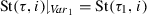• and ${{\,\mathrm{St}\,}}(\tau ,i){\downharpoonright _{ Var _2}} = {{\,\mathrm{St}\,}}(\tau _2,i)$ for $0 \le i \le |\tau |$

• ${{\,\mathrm{Loc}\,}}(\tau ,i) = \big ({{\,\mathrm{Loc}\,}}(\tau _1,i),{{\,\mathrm{Loc}\,}}(\tau _2,i)\big )$ for $0 \le i \le |\tau |$

• for $1 \le i \le |\tau |$, one of the following hold:

  • ${{\,\mathrm{Ag}\,}}(\tau _1, i) = 1$, ${{\,\mathrm{Ag}\,}}(\tau _2, i) = \mathsf {e}$, and ${{\,\mathrm{Ag}\,}}(\tau , i) = 1$

  • ${{\,\mathrm{Ag}\,}}(\tau _1, i) = \mathsf {e}$, ${{\,\mathrm{Ag}\,}}(\tau _2, i) = 1$, and ${{\,\mathrm{Ag}\,}}(\tau , i) = 2$

  • ${{\,\mathrm{Ag}\,}}(\tau _1, i) = \mathsf {e}$, ${{\,\mathrm{Ag}\,}}(\tau _2, i) = \mathsf {e}$, and ${{\,\mathrm{Ag}\,}}(\tau , i) = \mathsf {e}$

Lemma 2

(Compositionality of trace semantics) Let $P_1,S_1$ and $P_2,S_2$ be programs and predicates such that $P_1 \parallel P_2$ is defined. Then ${{\,\mathrm{traces}\,}}(S_1\wedge S_2,P_1\parallel P_2) = \{ \tau \mid \text {there exist } \tau _1\in {{\,\mathrm{traces}\,}}(S_1,P_1) \text { and } \tau _2\in {{\,\mathrm{traces}\,}}(S_2,P_2) \text { such that } \tau \propto \tau _1 \parallel \tau _2 \}$.

Proof

From Definitions 2 and 14. $\square$

Lemma 3

(Soundness of Par) Rule Par in Fig. 3 is sound.

Proof

Let $P_1$ and $P_2$ be programs such that $P_1 \parallel P_2$ is defined. We assume

(15)

(16)

and show

(17)

Let $\tau \in {{\,\mathrm{traces}\,}}(S_1\wedge S_2, P_1\parallel P_2)$ such that $\tau {\downharpoonright _{\{\mathsf {e}\}}} \models _{\sigma _0} \mathcal {R}$ where $\sigma _0 \in \llbracket S_1 \wedge S_2 \rrbracket$ is the initial state of $\tau$. By Lemma 2 we have that there exist traces $\tau _1 \in {{\,\mathrm{traces}\,}}(S,P_1)$, $\tau _2\in {{\,\mathrm{traces}\,}}(S,P_2)$ such that $\tau \propto \tau _1 \parallel \tau _2$.

We first show that $P_1 \parallel P_2$ satisfies the guarantee $(\mathcal {G}_1, \mathcal {G}_2)$. The proof proceeds by induction on the length of $\tau$.

Base case: $\tau$ is empty ($|\tau | = 0$). Then by Definition 14$\tau _1$ is empty and $\tau {\downharpoonright _{\{1\}}} \models _{\sigma _0} \mathcal {G}_1$ trivially holds. $\mathcal {G}_2$ by symmetry.

Step case: Suppose $\tau$ is non-empty ($|\tau |>0$) and rule Par is sound for traces of length $|\tau |-1$. From $S_1 \wedge S_2 \Rightarrow S_1$ we have $\sigma _0 \in \llbracket S_1 \rrbracket$. $\sigma _0 \in \llbracket S_2 \rrbracket$ by symmetry. We case split on the labeling of the last transition of $\tau _1$. Suppose it is $\mathsf {e}$, then $\tau {\downharpoonright _{\{1\}}} \models _{\sigma _0} \mathcal {G}_1$ follows immediately from (15) and the induction hypothesis. Suppose it is 1. By Definition 14, $\tau _2$’s last transition is labeled $\mathsf {e}$, and $\tau _2{\downharpoonright _{\{1\}}} \models _{\sigma _0} \mathcal {G}_2$ follows from the induction hypothesis. By Definition 14, the $\mathsf {e}$-transitions of $\tau _1$ are either $\mathsf {e}$-transitions of $\tau$ or 1-transitions of $\tau _2$. About these we have $\tau {\downharpoonright _{\{\mathsf {e}\}}} \models _{\sigma _0} \mathcal {R}$ (from the initial assumption) and $\tau _2{\downharpoonright _{\{1\}}} \models _{\sigma _0} \mathcal {G}_2$ (above). Then $\tau _1{\downharpoonright _{\{\mathsf {e}\}}} \models _{\sigma _0} \mathcal {R}+ \mathcal {G}_2$ and from (15) by Definition 10$\tau _1{\downharpoonright _{\{1\}}} \models _{\sigma _0} \mathcal {G}_1$. Thus $\tau {\downharpoonright _{\{1\}}} \models _{\sigma _0} \mathcal {G}_1$. $\mathcal {G}_2$ by symmetry.

It remains to show that $P_1 \parallel P_2$ satisfies the postcondition $S_1' \wedge S_2'$. Assume $\tau$ is finite and ends in $((\ell _1',\ell _2'),\sigma ')$. We show that $\sigma ' \ne \bot$ and $\sigma ' \models S_1'\wedge S_2'$: By Definition 14, $\tau _i$ is finite and ends in $(\ell _i',\sigma '{\downharpoonright _{ Var _i}})$ for $i\in \{1,2\}$. From (15) and (16) by Definition 10 we have that $\sigma '{\downharpoonright _{ Var _i}} \ne \bot$ and $\sigma '{\downharpoonright _{ Var _i}} \in \llbracket S_i' \rrbracket$. Thus $\sigma ' \ne \bot$ and $\sigma ' \in \llbracket S_1' \wedge S_2' \rrbracket$. $\square$

Lemma 4

(Soundness of Par-Merge) Rule Par-Merge in Fig. 3 is sound.

Proof

We assume

(18)

and show

(19)

Let $\tau \in {{\,\mathrm{traces}\,}}(S,P_1\parallel P_2)$ such that $\tau {\downharpoonright _{\{\mathsf {e}\}}} \models _{\sigma _0} \mathcal {R}$ where $\sigma _0 \in \llbracket S \rrbracket$ is the initial state of $\tau$. Let $\tau '$ be $\tau$ where all 1-transitions corresponding to transitions of $P_2$ are re-labeled with 2. By construction, $\tau '{\downharpoonright _{\{\mathsf {e}\}}} \models _{\sigma _0} \mathcal {R}$. From this and (18) by Definition 10, we have $\tau '{\downharpoonright _{\{1\}}} \models _{\sigma _0} \mathcal {G}_1$ and $\tau '{\downharpoonright _{\{2\}}} \models _{\sigma _0} \mathcal {G}_2$, thus $\tau '{\downharpoonright _{\{1,2\}}} \models _{\sigma _0} \mathcal {G}_1 + \mathcal {G}_2$, and thus $\tau {\downharpoonright _{\{1\}}} \models _{\sigma _0} \mathcal {G}_1 + \mathcal {G}_2$.

Suppose $\tau$ is finite. Then so is $\tau '$ and from (18) by Definition 10, we have that $\tau '$ ends in $(\ell ',\sigma ')$ where $\sigma ' \ne \bot$ and $\sigma ' \in \llbracket S' \rrbracket$. By construction, the same holds for $\tau$. $\square$

Lemma 5

(Soundness of Conseq) Rule Conseq in Fig. 3 is sound.

Proof

Case 1 (total guarantee, i.e., $\vec {\mathcal {G}}_i = \mathcal {G}_i$): We assume

(20)

(21)

and show

(22)

Let $\tau \in {{\,\mathrm{traces}\,}}(S_2,P)$ such that $\tau {\downharpoonright _{\{\mathsf {e}\}}} \models _{\sigma _0} \mathcal {R}_2$ where $\sigma _0 \in \llbracket S_2 \rrbracket$ is the initial state of $\tau$. From assumption $S_2 \Rightarrow S_1$ we have that $\tau \in {{\,\mathrm{traces}\,}}(S_1,P)$ and $\sigma _0 \in \llbracket S_1 \rrbracket$. From $\mathcal {R}_2 \subseteq _{S_2} \mathcal {R}_1$ it follows that $\tau {\downharpoonright _{\{\mathsf {e}\}}} \models _{\sigma _0} \mathcal {R}_1$. From this and (2021) by Definition 10 we have $\tau {\downharpoonright _{\{1\}}} \models _{\sigma _0} \mathcal {G}_1$; together with assumption $\mathcal {G}_1 \subseteq _{S_2} \mathcal {G}_2$ it follows that $\tau {\downharpoonright _{\{1\}}} \models _{\sigma _0} \mathcal {G}_2$. From (2021) by Definition 10 we have that if $\tau$ is finite and ends in $(\ell ',\sigma ')$ for some $\ell '$, then $\sigma ' \ne \bot$ and $\sigma ' \in \llbracket S_1' \rrbracket$. By assumption $S_1' \Rightarrow S_2'$, we have $\sigma ' \in \llbracket S_2' \rrbracket$.

Case 2 (thread-specific guarantee, i.e., $\vec {\mathcal {G}}_i = (\mathcal {G}_{i,1}, \mathcal {G}_{i,2})$): We assume

(23)

(24)

(25)

and show

(26)

Let $\tau \in {{\,\mathrm{traces}\,}}(S_2, P_1 \parallel P_2)$ such that $\tau {\downharpoonright _{\{\mathsf {e}\}}} \models _{\sigma _0} \mathcal {R}_2$ $\sigma _0 \in \llbracket S_2 \rrbracket$ is the initial state of $\tau$. From $S_2 \Rightarrow S_1$ we have that $\tau \in {{\,\mathrm{traces}\,}}(S_1,P_1 \parallel P_2)$ and $\sigma _0 \in \llbracket S_1 \rrbracket$. From assumption $\mathcal {R}_2 \subseteq _{S_2} \mathcal {R}_1$ we have $\tau {\downharpoonright _{\{\mathsf {e}\}}} \models _{\sigma _0} \mathcal {R}_1$. From (232425) by Definition 10 we have $\tau {\downharpoonright _{\{i\}}} \models _{\sigma _0} \mathcal {G}_{1,i}$ for $i\in \{1,2\}$ and thus by assumption $\mathcal {G}_{1,i} \subseteq _{S_2} \mathcal {G}_{2,i}$ we have $\tau {\downharpoonright _{\{i\}}} \models _{\sigma _0} \mathcal {G}_{2,i}$. From (232425) by Definition 10 we have that if $\tau$ is finite and ends in $(\ell ',\sigma ')$ for some $\ell '$, then $\sigma ' \ne \bot$ and $\sigma ' \in \llbracket S_1' \rrbracket$. By assumption $S_1' \Rightarrow S_2'$, we have $\sigma ' \in \llbracket S_2' \rrbracket$. $\square$

Theorem 1

(Soundness) The rules in Fig. 3 are sound.

Proof

From Lemmas 3, 4, 5. $\square$

1.2 B Proof of Theorem 2

Theorem 2

(Generalization of single-thread guarantees to N Threads) Let P be a program over local and shared variables $Var = LVar \cup SVar$ and let $\Vert _N P = P_1 \parallel \dots \parallel P_N$ be its N-times interleaving. Let S be a predicate over $SVar$. Let $\mathcal {A}$ over $SVar$ be a sound set of effect summaries for P started from S, and let $\mathcal {R}$ and $\mathcal {G}$ be environment assertions over $\mathcal {A}$. Let $\mathbf {0} = (0,\dots ,0)$ denote the empty environment.

If

then

I.e., if $(N-1) \times \mathcal {G}$ is smaller than $\mathcal {R}$, and if holds, then in an empty environment, $P_1$’s environment $P_2\parallel \dots \parallel P_N$ executes effect summaries $\mathcal {A}$ no more than $(N-1)\times \mathcal {G}$ times.

Proof

Note that proving the conclusion above is (by symmetry of threads $P_1,\dots ,P_N$) equivalent to moving the parentheses and proving

(27)

We show the stronger property that for all $k \ge 2$ and all $N \ge k$

(28)

Then for $k = N$ we prove our goal. The proof proceeds by induction on k:

Base case: $k=2$. We assume the premises of Theorem 2

(29)

(30)

hold, and show

(31)

By side condition (29) we apply rule Conseq to (30) to weaken the rely to $(N-1)\times \mathcal {G}$, yielding

(32)

By symmetry, (32) also holds for $P_2$:

(33)

By Lemma 1, $\mathcal {A}$ still over-approximates the effects of $P_1 \parallel P_2$. We apply rule Par to (32) and (33) and obtain the proof goal for the base case

(34)

Step case: If $N=k$, then we are done. Assume $N>k$. We start by applying Par-Merge to the induction hypothesis

(35)

to obtain

(36)

By symmetry, (32) also holds for $P_{k+1}$:

(37)

By Corollary 1, $\mathcal {A}$ still over-approximates $P_1 \parallel \dots \parallel P_{k+1}$. We apply Par to (36) and (37) and obtain the proof goal for the step case

(38)

$\square$

References

Abadi M, Lamport L (1995) Conjoining specifications. ACM Trans. Program. Lang. Syst. 17(3):507–534
Abdulla PA, Haziza F, Holík L, Jonsson B, Rezine A (2013) An integrated specification and verification technique for highly concurrent data structures. In: TACAS, Lecture Notes in Computer Science, vol. 7795, pp. 324–338. Springer
Albert E, Arenas P, Genaim S, Gómez-Zamalloa M, Puebla G (2012) Automatic inference of resource consumption bounds. In: LPAR, Lecture Notes in Computer Science, vol. 7180, pp. 1–11. Springer
Albert E, Arenas P, Genaim S, Puebla G (2011) Closed-form upper bounds in static cost analysis. J. Autom. Reason. 46(2):161–203
Albert E, Flores-Montoya A, Genaim S, Martin-Martin E (2017) Rely-guarantee termination and cost analyses of loops with concurrent interleavings. J. Autom. Reason. 59(1):47–85
Alias C, Darte A, Feautrier P, Gonnord L (2010) Multi-dimensional rankings, program termination, and complexity bounds of flowchart programs. In: SAS, Lecture Notes in Computer Science, vol. 6337, pp. 117–133. Springer
Berdine J, Lev-Ami T, Manevich R, Ramalingam G, Sagiv S (2008) Thread quantification for concurrent shape analysis. In: CAV, Lecture Notes in Computer Science, vol. 5123, pp. 399–413. Springer
Bouajjani A, Bozga M, Habermehl P, Iosif R, Moro P, Vojnar T (2011) Programs with lists are counter automata. Formal Methods Syst. Des. 38(2):158–192
Brockschmidt M, Emmes F, Falke S, Fuhs C, Giesl J (2016) Analyzing runtime and size complexity of integer programs. ACM Trans. Program. Lang. Syst. 38(4):13:1-13:50
Calcagno C, Distefano D, O’Hearn PW, Yang H (2009) Compositional shape analysis by means of bi-abduction. In: POPL, pp. 289–300. ACM
Calcagno C, Parkinson MJ, Vafeiadis V (2007) Modular safety checking for fine-grained concurrency. In: SAS,Lecture Notes in Computer Science, vol. 4634, pp. 233–248. Springer
Carbonneaux Q, Hoffmann J, Reps TW, Shao Z (2017) Automated resource analysis with coq proof objects. In: CAV (2), Lecture Notes in Computer Science, vol. 10427, pp. 64–85. Springer
Chakraborty S, Henzinger TA, Sezgin A, Vafeiadis V (2015) Aspect-oriented linearizability proofs. Logical Methods Comput Sci 11(1)
Coachman. https://github.com/thpani/coachman (2019)
Cook B, Podelski A, Rybalchenko A (2007) Proving thread termination. In: PLDI, pp. 320–330. ACM
Doherty S, Groves L, Luchangco V, Moir M (2004) Formal verification of a practical lock-free queue algorithm. In: FORTE, Lecture Notes in Computer Science, vol. 3235, pp. 97–114. Springer
Fiedor T, Holík L, Rogalewicz A, Sinn M, Vojnar T, Zuleger F (2018) From shapes to amortized complexity. In: VMCAI, Lecture Notes in Computer Science, vol. 10747, pp. 205–225. Springer
Flanagan C, Freund SN, Qadeer S (2002) Thread-modular verification for shared-memory programs. In: ESOP, Lecture Notes in Computer Science, vol. 2305, pp. 262–277. Springer
Flanagan C, Qadeer S (2003) Thread-modular model checking. In: SPIN, Lecture Notes in Computer Science, vol. 2648, pp. 213–224. Springer
Flores-Montoya A, Hähnle R (2014) Resource analysis of complex programs with cost equations. In: APLAS, Lecture Notes in Computer Science, vol. 8858, pp. 275–295. Springer
Gotsman A, Berdine J, Cook B, Sagiv M (2007) Thread-modular shape analysis. In: PLDI, pp. 266–277. ACM
Gotsman A, Cook B, Parkinson MJ, Vafeiadis V (2009) Proving that non-blocking algorithms don’t block. In: POPL, pp. 16–28. ACM
Gulwani S, Zuleger F (2010) The reachability-bound problem. In: PLDI, pp. 292–304. ACM
Hendler D, Shavit N, Yerushalmi L (2004) A scalable lock-free stack algorithm. In: SPAA, pp. 206–215. ACM
Herlihy M, Shavit N (2008) The art of multiprocessor programming. Morgan Kaufmann, USA
Holík L, Meyer R, Vojnar T, Wolff S (2017) Effect summaries for thread-modular analysis - sound analysis despite an unsound heuristic. In: SAS, Lecture Notes in Computer Science, vol. 10422, pp. 169–191. Springer
Jia X, Li W, Vafeiadis V (2015) Proving lock-freedom easily and automatically. In: CPP, pp. 119–127. ACM
Jones CB (1983) Specification and design of (parallel) programs. In: IFIP Congress, pp. 321–332. North-Holland/IFIP
Malkis A, Podelski A, Rybalchenko A (2006) Thread-modular verification is cartesian abstract interpretation. In: ICTAC, Lecture Notes in Computer Science, vol. 4281, pp. 183–197. Springer
McMillan KL (1999) Circular compositional reasoning about liveness. In: CHARME, Lecture Notes in Computer Science, vol. 1703, pp. 342–345. Springer
Michael MM, Scott ML (1996) Simple, fast, and practical non-blocking and blocking concurrent queue algorithms. In: PODC, pp. 267–275. ACM
Miné A (2011) Static analysis of run-time errors in embedded critical parallel C programs. In: ESOP, Lecture Notes in Computer Science, vol. 6602, pp. 398–418. Springer
Pani T, Weissenbacher G, Zuleger F (2018) Rely-guarantee reasoning for automated bound analysis of lock-free algorithms. In: FMCAD, pp. 1–9. IEEE
Petrank E, Musuvathi M, Steensgaard B (2009) Progress guarantee for parallel programs via bounded lock-freedom. In: PLDI, pp. 144–154. ACM
Reynolds JC (2002) Separation logic: A logic for shared mutable data structures. In: LICS, pp. 55–74. IEEE Computer Society
Sinn M, Zuleger F, Veith H (2017) Complexity and resource bound analysis of imperative programs using difference constraints. J. Autom. Reason 59(1):3–45
Ströder T, Giesl J, Brockschmidt M, Frohn F, Fuhs C, Hensel J, Schneider-Kamp P, Aschermann C (2017) Automatically proving termination and memory safety for programs with pointer arithmetic. J. Autom. Reason 58(1):33–65
Treiber RK (1986) Systems programming: Coping with parallelism. Tech. Rep. RJ 5118, IBM Almaden Research Center
Vafeiadis V (2009) Shape-value abstraction for verifying linearizability. In: VMCAI, Lecture Notes in Computer Science, vol. 5403, pp. 335–348. Springer
Vafeiadis V (2010) Automatically proving linearizability. In: CAV, Lecture Notes in Computer Science, vol. 6174, pp. 450–464. Springer
Vafeiadis V (2010) Rgsep action inference. In: VMCAI, Lecture Notes in Computer Science, vol. 5944, pp. 345–361. Springer
Xu Q, de Roever WP, He J (1997) The rely-guarantee method for verifying shared variable concurrent programs. Formal Asp. Comput. 9(2):149–174
Acknowledgements
We would like to thank Erez Petrank, Ana Sokolova, and the anonymous reviewers for comments and discussions that helped to improve this paper.
Funding
Open access funding provided by TU Wien (TUW).
Author information
Authors and Affiliations
Corresponding author
Additional information
Publisher's Note
Springer Nature remains neutral with regard to jurisdictional claims in published maps and institutional affiliations.