Angled Crested Like Water Waves with Surface Tension: Wellposedness of the Problem

Abstract

We consider the capillary–gravity water wave equation in two dimensions. We assume that the fluid is inviscid, incompressible, irrotational and the air density is zero. We construct an energy functional and prove a local wellposedness result without assuming the Taylor sign condition. When the surface tension $\sigma$ is zero, the energy reduces to a lower order version of the energy obtained by Kinsey and Wu (Camb J Math 6(2):93–181, 2018) and allows angled crest interfaces. For positive surface tension, the energy does not allow angled crest interfaces but admits initial data with large curvature of the order of $\sigma ^{-\frac{1}{3}+ \epsilon }$ for any $\epsilon >0$.

Appendix

Here we will prove all the identities and estimates used in the paper. We will state most of the statements only for functions in the Schwartz class and it can be extended to more general functions by an approximation argument. Let us first recall some of the notation used. Let $D_t= \partial _t+ b\partial _{\alpha '}$ where $b$ is given by (11) and recall that is defined as

Proposition 9.1

Let $f,g,h \in \mathcal {S}(\mathbb {R})$. Then we have the following identities

• (1)
• (2)

Proof

The second identity is a direct consequence of the first. Now we see that

$\square$

Proposition 9.2

Let $H \in C^1(\mathbb {R}),A_i \in C^1(\mathbb {R})$ for $i=1,\cdots m$ and $F\in C^\infty (\mathbb {R})$. Define

then there exists constants $c_1,c_2,c_3,c_4$ depending only on F and so that

• (1)
• (2)
• (3)
• (4)

Proof

The first estimate is a theorem by Coifman, McIntosh and Meyer [15]. See also chapter 9 of [29]. Estimate 2 is a consequence of the Tb theorem and a proof can be found in [43]. The third and fourth estimates can be obtained from the first two by integration by parts. $\quad \square$

Proposition 9.3

Let $T:\mathcal {D}(\mathbb {R}) \rightarrow \mathcal {D}'(\mathbb {R})$ be a linear operator with kernel K(x, y) such that on the open set $\{(x,y):x\ne y\} \subset \mathbb {R}\times \mathbb {R}$, K(x, y) is a function satisfying

where $C_0$ is a constant. If T is continuous on $L^2(\mathbb {R})$ with and if $T(1) =0$, then T is bounded on $\dot{H}^s$ for $0<s<1$ with

Proof

This proposition is a direct consequence of the result of Lemarie [25] where only weak boundedness of T on $L^2$ (in the sense of David and Journe) is assumed. As boundedness on $L^2$ implies weak boundedness, the proposition follows. See also chapter 10 of [29] for another proof of the result of Lemarie. $\quad \square$

Lemma 9.4

Let $r,s \in \mathbb {R}$, $k,m\in \mathbb {Z}$. If $f \in \mathcal {S}(\mathbb {R})$, then we have the following

• (1)    for $0\le r<s$ with $1-\theta = \frac{r}{s}$

• (2)    for $2\le r<s$ with $1-\theta = \frac{r-2}{s-2}$

• (3)    for $0\le k <m$ with $1-\theta = \frac{k+\frac{1}{2}}{m}$

• (4)    for $2\le k <m$ with $1-\theta = \frac{k-\frac{3}{2}}{m-2}$

Proof

The first estimate is a standard interpolation estimate which can be easily proved by using the Fourier transform. We skip its proof. The second one follows from the first by applying it on the function $f''$ with r, s replaced by $r-2,s-2$ respectively.

The third estimate is a consequence of the Gagliardo-Nirenberg interpolation estimate (see Theorem 12.87 in [26]). The last one follows from the third estimate by applying it on the function $f''$ with k, m replaced by $k-2,m-2$ respectively. $\quad \square$

Lemma 9.5

Let $k,n \in \mathbb {N}$ and $f_1,f_2, \cdots , f_k \in \mathcal {S}(\mathbb {R})$. Let $r_1,r_2\cdots , r_k \in \mathbb {Z}$ with $r_1 + \cdots + r_k = n$ and $r_i\ge 0$ for all $1\le i\le k$ and. Let . Then

• (1)    for

• (2)    for

with and C(K) is a constant depending only on K.

Proof

Let us begin by proving the first estimate. Without loss of generality $0\le r_1\le r_2 \le \cdots \le r_k$. Clearly the estimate holds if $k=1$ or $r=1$. Hence we can now assume that $k\ge 2$ and $r\ge 2$. If $r_1\le \cdots \le r_j \le 1$ for some $j<k$ with $r_{j+1} \ge 2$, then we have

Hence without loss of generality we can assume that $r_1\ge 2$. As $k\ge 2$ this implies that $n\ge 4$ and we also have $r\ge 2$, $r\le n-2$ and $s = n-2$. Hence using Lemma 9.4 we have

where $1-\theta _j = \frac{r_j - \frac{3}{2}}{s-1}$ for $j<k$ and $1-\theta _k = \frac{r_k - 2}{s-1}$. Now observe that

$$\begin{aligned} (1-\theta _1) + \cdots + (1-\theta _k) = \frac{r_1 - \frac{3}{2}}{s-1} + \cdots + \frac{r_{k-1} - \frac{3}{2}}{s-1} + \frac{r_k - 2}{s-1} \le 1 \end{aligned}$$

Hence by using $AM-GM$ inequality the estimate follows. The proof of the second estimate is very similar and we skip it. $\quad \square$

Corollary 9.6

Let $f,g \in \mathcal {S}(\mathbb {R})$ and let $n\in \mathbb {N}$ with $n\ge 2$. Then

• (1) for $s = n-2$

• (2) for $s = n-\frac{3}{2}$

where and C(K) is a constant depending only on K.

Proof

This follows directly from Lemma 9.5$\quad \square$

Proposition 9.7

Let $f \in \mathcal {S}(\mathbb {R})$. Then we have

• (1) if $s>\frac{1}{2}$ and for $s=\frac{1}{2}$ we have

• (2)
• (3)
• (4)
• (5)

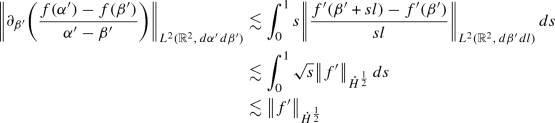
Proof

• (1) This is a standard Sobolev embedding result.

• (2) This is a consequence of Hardy’s inequality.

• (3) We see that

  

  where M is the uncentered Hardy Littlewood maximal operator. As the maximal operator is bounded on $L^2$, the estimate follows.

• (4) Observe that as $\vert {\partial _{\alpha '}}\vert = i\mathbb {H}\partial _{\alpha '}$ and $\mathbb {H}(1) =0$ we have

  

  Now observe that

  

  The identity now follows.

• (5) We see that

  

  Hence we have

  

$\square$

Proposition 9.8

Let $f,g \in \mathcal {S}(\mathbb {R})$ with $s,a\in \mathbb {R}$ and $m,n \in \mathbb {Z}$. Then we have the following estimates

• (1)    for $s,a \ge 0$

• (2)    for $s\ge 0$ and $a>0$

• (3)
• (4)

• (5)    for $m,n \ge 0$

• (6)    for $m,n \ge 0$

• (7)    for $m\ge 0$ and $n\ge 1$

• (8)

Proof

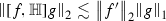
The first four estimates are all variants of the Kato Ponce commutator estimate and are proved using the paraproduct decomposition. See Lemma 2.1 in [20] for the first two estimates and Theorem 1.2 in [27] for the third and fourth estimates. The fourth estimate is not explicitly stated as part of Theorem 1.2 in [27] however the proof is identical to the proof of estimate 3 with the only change being at the last step where you move half a derivative from g to f.

The $\dot{H}^\frac{1}{2}$ estimate of the fifth estimate follows from the first estimate. For the $L^{\infty }$ estimate note that

The estimate now follows from the Cauchy Schwarz inequality. The sixth and seventh estimates follow from the first two estimates. For the last estimate observe that

The estimate now follows from Hardy’s inequality as stated in Proposition 9.7. $\quad \square$

Proposition 9.9

Let $f,g,h \in \mathcal {S}(\mathbb {R})$ with $s,a\in \mathbb {R}$ and $m,n \in \mathbb {Z}$. Then we have the following estimates

• (1)    for $s > 0$

• (2)
• (3)

Proof

See [22] for the first estimate. The second one is a special case of the first. For the third one observe that

and hence from Proposition 9.8

$\square$

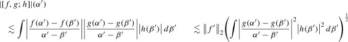
Proposition 9.10

Let $f,g,h \in \mathcal {S}(\mathbb {R})$ . Then we have the following estimates

• (1)
• (2)
• (3)
• (4)
• (5)

Proof

• (1) We see that

  

  The estimate now follows from Hardy’s inequality.

• (2) We see that

  

  The estimate now follows by previous estimates.

• (3) This is a special case of Proposition 9.2

• (4) From the third estimate we observe that the operator T defined by the action is bounded on $L^2$. Also we clearly see that $T(1) =0$. It is also easy to see that the kernel of this operator satisfies the conditions for Proposition 9.3. Hence the operator T is bounded on $\dot{H}^\frac{1}{2}$.

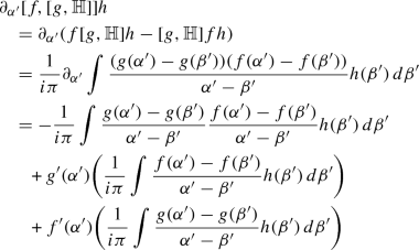
• (5) The $L^{\infty }$ estimate is obtained easily by an application of Cauchy Schwarz and Hardy’s inequality. Now we use and see that

  

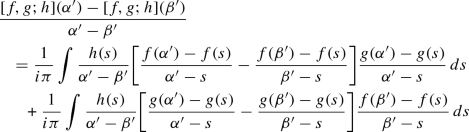
  Now we use the following notation to simplify the calculation

  $$\begin{aligned} F(a,b) = \frac{f(a) -f(b)}{a-b} \quad \text { and } G(a,b) = \frac{g(a)-g(b)}{a-b} \end{aligned}$$

  Hence we have

  

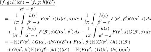
  and we see that

  

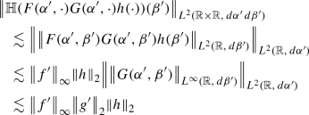
  The other terms are handled similarly.$\quad \square$

Proposition 9.11

Let $f \in \mathcal {S}(\mathbb {R})$ and let w be a smooth non-zero weight with $w,\frac{1}{w} \in L^{\infty }(\mathbb {R})$ and $w' \in L^2(\mathbb {R})$. Then

• (1)
• (2)

Proof

• (1) We see that

  

  Now we integrate and use Cauchy Schwarz to get the estimate.

• (2) The $L^{\infty }$ estimate is obtained from the first estimate by observing that

  

Now use the inequality $ab \le \frac{a^2}{2\epsilon } + \frac{\epsilon b^2}{2}$ on the last term to obtain the estimate. For the $\dot{H}^\frac{1}{2}$ estimate, using $\vert {\partial _{\alpha '}}\vert = i\mathbb {H}\partial _{\alpha '}$ we see that

Now as we have

$$\begin{aligned} s \end{aligned}$$

Hence using the inequality $ab \le \frac{a^2}{2} + \frac{b^2}{2}$, we see that

$\quad \square$

Proposition 9.12

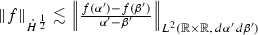
Let $f,g \in \mathcal {S}(\mathbb {R})$ and let $w,h \in L^{\infty }(\mathbb {R})$ be smooth functions with $w',h' \in L^2(\mathbb {R})$. Then

If in addition we assume that w is real valued then

Proof

• (1) We see that

  

  The estimate now follows from the estimate

• (2) We observe that

  $$\begin{aligned} fgw&= (\mathbb {P}_Hf)(\mathbb {P}_Hg)w + (\mathbb {P}_Hf)(\mathbb {P}_Ag)w + (\mathbb {P}_Af)(\mathbb {P}_Hg)w + (\mathbb {P}_Af)(\mathbb {P}_Ag)w \\&= (\mathbb {P}_Hf)\overline{(\mathbb {P}_A\bar{g})}w + (\mathbb {P}_Hf)(\mathbb {P}_Ag)w + (\mathbb {P}_Af)(\mathbb {P}_Hg)w + (\mathbb {P}_Af)\overline{(\mathbb {P}_H\bar{g})}w \end{aligned}$$

We will control only the first term and the other terms are controlled similarly. Now see that

Hence we have

Now observe that as w is real valued we have

Similarly we have

$\square$

Proposition 9.13

Let $f \in C^3([0,T), H^3(\mathbb {R}))$. Then for any $t\in [0,T)$ we have

Proof

Fix $s > 0$ satisfying $t+s \in [0,T)$ and for every $\epsilon >0$ we find $a_{\epsilon } \in \mathbb {R}$ such that . Observe that and hence we have

Now let $\epsilon \rightarrow 0$ to get

As $\partial _t^2 f \in L^{\infty }(\mathbb {R}\times [0,T))$, we take the limit as $s\rightarrow 0$ to finish the proof. $\quad \square$

Lemma 9.14

Let $K_\epsilon$ be the Poisson kernel from (3). If $f\in L^q(\mathbb {R})$, then for $s\ge 0$ an integer we have

Similarly for $s \in \mathbb {R}, s\ge 0$ we have

Proof

The proof follows from basic properties of convolution. $\quad \square$