Distributed arrays: an algebra for generic distributed query processing

Abstract

We propose a simple model for distributed query processing based on the concept of a distributed array. Such an array has fields of some data type whose values can be stored on different machines. It offers operations to manipulate all fields in parallel within the distributed algebra. The arrays considered are one-dimensional and just serve to model a partitioned and distributed data set. Distributed arrays rest on a given set of data types and operations called the basic algebra implemented by some piece of software called the basic engine. It provides a complete environment for query processing on a single machine. We assume this environment is extensible by types and operations. Operations on distributed arrays are implemented by one basic engine called the master which controls a set of basic engines called the workers. It maps operations on distributed arrays to the respective operations on their fields executed by workers. The distributed algebra is completely generic: any type or operation added in the extensible basic engine will be immediately available for distributed query processing. To demonstrate the use of the distributed algebra as a language for distributed query processing, we describe a fairly complex algorithm for distributed density-based similarity clustering. The algorithm is a novel contribution by itself. Its complete implementation is shown in terms of the distributed algebra and the basic algebra. As a basic engine the Secondo system is used, a rich environment for extensible query processing, providing useful tools such as main memory M-trees, graphs, or a DBScan implementation.

1 Introduction

Big data management has been a core topic in research and development for the last fifteen years. Its popularity was probably started by the introduction of the MapReduce paradigm [10] which allowed a simple formulation of data processing tasks by a programmer which are then executed in a highly scalable and fault tolerant way on a large set of machines. Massive data sets arise through the global scale of the internet with applications and global businesses such as Google, Amazon, Facebook. Other factors are the ubiquity of personal devices collecting and creating all kinds of data, but also the ever growing detail of scientific experiments and data collection, for example, in physics or astronomy, or the study of the human brain or the genome.

Dealing with massive data sets requires to match the size of the problem with a scalable amount of resources; therefore distributed and parallel processing is essential. Following MapReduce and its open source version Hadoop, many frameworks have been developed, for example, Hadoop-based approaches such as HadoopDB, Hive, Pig; Apache Spark and Flink; graph processing frameworks such as Pregel or GraphX.

All of these systems provide some model of the data that can be manipulated and a language for describing distributed processing. For example, MapReduce/Hadoop processes key-value pairs; Apache Spark offers resilient distributed data sets in main memory; Pregel manipulates nodes and edges of a graph in a node-centric view. Processing is described in terms of map and reduce functions in Hadoop; in an SQL-like style in Hive; by a set of operations on tables in Pig; by a set of operations embedded in a programming language environment in Spark; or by functions processing messages between nodes in Pregel.

In this paper, we consider the problem of transforming an extensible query processing system on a single machine (called the basic engine) into a scalable parallel query processing system on a cluster of computers. All the capabilities of the basic engine should automatically be available for parallel and distributed query processing, including extensions to the local system added in the future.

We assume the basic engine implements an algebra for query processing called the basic algebra. The basic algebra offers some data types and operations. The basic engine allows one to create and delete databases and within databases to create and delete objects of data types of the basic algebra. It allows one to evaluate terms (expressions, queries) of the basic algebra over database objects and constants and to return the resulting values to the user or store them in a database object.

The idea to turn this into a scalable distributed system is to introduce an additional algebra for distributed query processing into the basic engine, the distributed algebra. The distributed system will then consist of one basic engine called the master controlling many basic engines called the workers. The master will execute commands provided by a user or application. These commands will use data types and operations of the distributed algebra. The types will represent data distributed over workers and the operations be implemented by commands and queries sent to the workers.

The fundamental conceptual model and data structure to represent distributed data is a distributed array. A distributed array has fields of some data type of the basic algebra; these fields are stored on different computers and assigned to workers on these computers. Queries are described as mappings from distributed arrays to distributed arrays. The mapping of fields is described by terms of the basic algebra that can be executed by the basic engines of the workers. Further, the distributed algebra allows one to distribute data from the master to the workers, creating distributed arrays, as well as collect distributed array fields from the workers to the master.

These ideas have been implemented in the extensible DBMS Secondo which takes the role of the basic engine. The Secondo kernel is structured into algebra modules each providing some data types and operations; all algebras together form the basic algebra. Secondo provides query processing over the implemented algebras as described above for the basic engine. Currently there is a large set of algebras providing basic data types (e.g., integer, string, bool, ...), relations and tuples, spatial data types, spatio-temporal types, various index structures including B-trees, R-trees, M-trees; data structures in main memory for relations, indexes, graphs; and many others. The distributed algebra described in this paper has been implemented in Secondo.

In the main part of this paper we design the data types and operations of the distributed algebra and formally define their semantics.

To illustrate distributed query processing based on this model, we describe an algorithm for distributed density-based similarity clustering. That is, we show the “source code” to implement the algorithm in terms of the distributed algebra and the basic algebra.

The contributions of the paper are as follows:

• A generic algebra for distributed query processing is presented.

• Data types and operations of the algebra are designed and their semantics are formally defined.

• The implementation of the distributed algebra is explained.

• A novel algorithm for distributed density-based similarity clustering is presented and its complete implementation in terms of the distributed algebra is shown.

• An experimental evaluation of the framework shows excellent load balancing and good speedup.

The rest of the paper is structured as follows. Related work is described in Sect. 2. In Sect. 3, Secondo as a generic extensible DBMS is introduced, providing a basic engine and algebra. In Sect. 4, the distributed algebra is defined. Sect. 5 describes the implementation of this algebra in Secondo. In Sect. 6 we show the algorithm for distributed clustering and its implementation. A brief experimental evaluation of the framework is given in Sect. 7. Finally, Sect. 8 concludes the paper.

2 Related work

Our algebra for generic distributed query processing in Secondo has related work in the areas of distributed systems, distributed databases, and data analytics. In the application section of this paper, we present an algorithm for the density-based similarity clustering (see Sect. 6). The most related work in these areas is discussed in this section.

2.1 Distributed system coordination

Developing a distributed software system is a complex task. Distributed algorithms have to be coordinated on several nodes of a cluster. Apache ZooKeeper [29], HashiCorp Consul [8] and etcd [16] are software components used to coordinate distributed systems. These systems cover topics such as service discovery and configuration management. Even these components are used in many software projects; some distributed computing engines have also implemented their own specialized resource management components (such as YARN—Yet Another Resource Negotiator [54], which is part of Hadoop).

In our distributed array implementation, we send the information to coordinate the system directly from the master node to the worker nodes. The worker nodes are manually managed in the current version of our implementation. Topics such as high availability or replication will be part of a further version.

2.2 Distributed file systems and distributed databases

2.2.1 General remarks

In this section we discuss systems for distributed analytical data processing.

A major distinction between those systems and the distributed algebra of this paper is genericity. The systems to be discussed all have some data model that is manipulated by operations, for example, tables or key-value pairs. In contrast, distributed algebra does not have any fixed data model. What is predetermined is the model of a distributed array which is just a simple abstraction of a partitioned (and distributed) data set. Furthermore, it is fixed that sets of tuples are used for data exchange. The field types of distributed arrays are absolutely generic.

This makes it possible to plug in a basic engine providing types and operations, if you want, a “legacy system”, with all its data structures and capabilities. The clear separation between the algebra describing distributed query processing and the basic algebra (or engine) defining local data and query processing by workers is unique for our approach.

Our implementation of the distributed algebra so far uses Secondo as a basic engine; we are currently working on embedding other systems, PostgreSQL in particular.

Many systems provide some level of extensibility such as user defined data types and functions. However, embedding a complete basic engine is a quite different matter: we simply inherit everything there is, without doing extra work for every part, as in the case of extensibility. The basic engine Secondo is a rich environment developed over many years. Beyond standard relational query processing it has specialized “algebra modules” for spatial and spatio-temporal data, index structures such as R-trees, TB-trees, M-trees, symbolic trajectories, image and raster data, map matching algorithms, DBScan, and so forth. There are persistent as well as main memory data structures, allowing distributed in-memory processing.

Moreover, the scope of extensibility within the basic engine Secondo is much higher than in other systems. Whereas in most systems user defined types can be added at the level of attribute types in tables, the architecture of Secondo is designed around extensibility. A DBMS data model is implemented completely in terms of algebra modules. Hence one can add not only atomic data types but also any kind of representation structure such as an index, a graph, or a column-oriented relation representation, for example.

In the following, we refer to Distributed Algebra as DA and to Distributed Algebra with Secondo as a basic engine as DA/Secondo, respectively.

2.2.2 MapReduce and distributed file systems

In 2004, the publication of the MapReduce paper [10] proposed a new technique for the distributed handling of computational tasks. Using MapReduce, calculations are performed in two phases: (1) a map phase and (2) a reduce phase. These tasks are executed on a cluster of nodes in a distributed and fault-tolerant manner. Map and reduce steps are formulated directly in a programming language.

The Google File System (GFS) [21] and its open-source counterpart Hadoop File System (HDFS) [45] are distributed file systems. These file systems represent the backbone of the MapReduce frameworks; they are used for the input and output of large datasets. Stored files are split up into fixed-sized chunks and distributed across a cluster of nodes. To deal with failing nodes, the chunks can be replicated. Due to the architecture of the file systems, data are stored in an append-only manner.

To exploit node level data locality, the MapReduce Master Node tries to schedule jobs in a way that the chunks of the input data are stored on the node that processes the data [21, p. 5]. If the chunks are stored on another node, the data need to be transferred over a network, which is slow and time-consuming. HDFS addresses data locality only on chunks and not based on the value of the stored data, which can lead to performance problems [14].

In our distributed array implementation, data are directly assigned to the nodes in a way that data locality is exploited, and the amount of transferred data is minimized. The output of a query can be directly partitioned and transferred to the worker nodes that are responsible for the next processing step (see the discussion of the $\underline{\smash { dfmatrix }}$ data type in Sect. 4). In addition, Secondo uses a type system. Before a query is executed, the query is checked for type errors. Therefore, in our distributed array implementation, the data are stored typed. On a distributed file system, data are stored as raw bytes. Type and structure information need to be implemented in the application that reads and writes the data.

2.2.3 Distributed databases and frameworks for analytic processing

HBase [27] (the open-source counterpart of BigTable [6]) is a distributed column-oriented database built on top of HDFS. HBase is optimized to handle large tables of data. Tables consist of rows of multiple column families (a set of key-value pairs). Internally, the data are stored in String Sorted Tables (SSTables) [6, 41], which are handled by HDFS. HBase provides simple operations to access the data (e.g., get and scan) and does not support complex operations such as joins; MapReduce jobs can be used to process the data. The DA can of course operate on data that is stored across a cluster of systems in a distributed manner. In addition, DA/Secondo offers a wide range of operators (such as joins), which can be used to process the data.

Key-Value Stores such as Amazon Dynamo [11] or RocksDB [49] provide a simple data model consisting of a key and a value. Systems such as HBase, BigTable, or Apache Cassandra [32] provide a slightly more complex data model. A key can have multiple values; internally, the data are stored as key-value pairs on disk. The values in these implementations are limited to scalar data types such as int, byte, or string.

Apache Hive [50] is a warehousing solution that is built on top of Apache Hadoop, which provides an SQL-like query language to process in HDFS stored data. Hive contains only a limited set of operations.

Apache Pig [18] provides a query language (called Pig Latin [40]) for processing large amounts of data. With Pig Latin, users no longer need to write their own MapReduce programs; they write queries which are directly translated into MapReduce jobs. Pig Latin focuses primarily on analytical workloads.

Pig Latin provides an interesting data model built from atomic types and tuples, bags and maps. Tuples may have flexible schemas and may be nested. A program is expressed as a sequence of assignments to variables, applying one operation in each step. Operations such as FILTER, FOREACH ... GENERATE, or COGROUP, JOIN, ORDER, can be applied to distributed data sets.

Comparing to DA, we find a fixed, not a generic data model. Operations on distributed data sets are tied to this model and perform implicit redistribution. In DA, we can nest operations (i.e., write sequences of operations) and we have a strict separation between distributed and local computation. Comparing to DA/Secondo, of course, the set of available data structures and operations is much more limited. For example, we do not have any indexes or index-based join algorithms.

Pigeon [13] is a spatial extension to Pig which supports spatial data types and operations. Pig was not extensible by atomic data types; any other type than number or string needed to be represented as bytearray. Hence the Pigeon extension represents spatial data types as Well-Known Text or Well-Known Binary exchange formats within Pig. Spatial functions need to convert from and to this format when working on the data.

Remarkable for a spatial extension is that there are no facilities for spatial indexing or spatial join. In the examples in [13], spatial join is expressed as cross product and filtering (CROSS and FILTER operators of PigLatin), a very inefficient evaluation. This is simply due to the fact that extensions by index structures or spatial join operators are not possible in the Pig framework.

In contrast, spatial data types, spatial indexing and spatial join are supported in DA/Secondo as demonstrated later in this paper.

The publication of the MapReduce paper created the foundation for many new applications and ideas to process distributed data. A widely used framework to process data in a scalable and distributed manner is Apache Spark [57]. In Spark, data are stored in resilient distributed datasets (RDDs) [56] in a distributed way across a cluster of nodes. In contrast to earlier work, RDDs can reside in memory in a fault-tolerant way. Hence Spark supports in particular distributed in-memory processing.

Spark defines an interesting set of operations on RDDs that may be compared to those of DA. For example, there is an operation (called transformation) $map(f: T =>U$), parameterized by a function mapping values of type T into those of type U. Applied to an RDD[T], i.e., an RDD with partitions of type U, it returns an RDD[U].

One can see that RDDs are generic and parameterized by types, hence they are fairly similar to the distributed arrays of this paper. Also the map transformation corresponds to our dmap operator, introduced later.

Differences are that RDDs and operations on them are not formalized, especially the way fields of RDDs are mapped to workers and are remapped by operations is determined only by the implementation. In DA, field indices do play a role, are controlled by a programmer and are part of the formalization. It is unclear whether in Spark the number of fields of an RDD can be chosen independently from the number of workers, as in DA. This is relevant for load balancing as shown later in the paper.

Another difference is that only some of the operations are generic; others assume types for key-value pairs or sequences. For example, groupByKey, join or cogroup transformations assume key-value pairs. In contrast, DA has only generic operations and all the transformation operations of RDDs can be expressed in DA/Secondo by combining DA operations with basic engine operations. How data are repartitioned is precisely defined in the DA.

Dryad [30] is a distributed execution engine that is developed at Microsoft. DryadLINQ [55] provides an interface for Dryad which can be consumed by Microsoft programming languages such as C#. In contrast to Secondo and our algebra implementation, the goal of Dryad is to provide a distributed environment for the parallel execution of user-provided programs such as Hadoop. The goal of our implementation is to provide an extensible environment with a broad range of predefined operators that can be used to progress data and which can also be enhanced with new operators by the user.

Another popular framework to process large amounts of data these days is Apache Flink [5]. This software system, originating from the Stratosphere Platform [1], is designed to handle batch and stream processing jobs. Processing batches (historical data or static data sets) is treated as a special form of stream processing. Data batches are processed in a time-agnostic fashion and handled as a bounded data stream. Like our system, Flink performs type checking and can be extended by user-defined operators and data types. However, Secondo ships with a larger amount of operators and data types. For example, it can handle spatial and spatio-temporal data out of the box.

Parallel Secondo [33] and Distributed Secondo [38] are two already existing approaches to execute queries in Secondo [24] in a distributed and parallel manner. Both approaches are integrating an existing software component into Secondo to achieve the distributed query execution. Parallel Secondo uses Apache Hadoop (the open source counterpart of the MapReduce framework) to distribute tasks over several Secondo installations on a cluster of nodes. Distributed Secondo uses Apache Cassandra as a distributed key-value store for the distributed storage of data, service discovery, and job scheduling. Both implementations use an additional component (Hadoop or Cassandra) to parallelize Secondo. The algebra for distributed arrays works without further components and provides the parallelization directly in Secondo.

2.3 Array databases and data frames

Array databases such as Rasdaman (raster data manager) [3], SciDB [47], or SciQL  [58] focus on the processing of data cubes (multi-dimensional arrays). In addition to specialized databases, there are raster data extensions for relational database management systems such as PostGIS Raster [44] or Oracle GeoRaster [42]. Array databases are used to process data like maps (two dimensional) or satellite image time series (three dimensional).

Our distributed array implementation works with one-dimensional arrays. The array is just used to structure the data for the workers, representing a partitioned distributed data set. Array databases use the dimensions of the array to represent the location of the data in the n-dimensional space, which is a different concept. Secondo works with index structures (such as the R-Tree [26]) for efficient data access. In addition, in array databases, the values of the array cells are restricted to primitive or common SQL types like integers or strings. In our model and implementation, the data types of the fields can be any type provided by the basic engine, hence an arbitrary type available in Secondo.

Libraries for processing array structured data (also called data frames), such as Pandas [36] or NumPy [39], are widely used in scientific computing these days. Such libraries are used to apply operations such as filters, calculations, or mutations on array structured data. SciHadoop [4] is using Hadoop to process data arrays in a distributed and parallel way. SciHive [19] is a system that uses Hive to process array structured data. AFrame [46] is another implementation of a data frame library which is built on top of Apache AsterixDB [2]. The goal of the implementation is to process the data frames in a distributed manner and hide the complexity of the distributed system from the user. These libraries and systems are intended for direct integration into the source code. These libraries simplify the handling of arrays, bring along data types and functions, and some also allow the distributed and parallel processing of arrays. Our system instead works with a query language to describe operator trees. Further, Secondo is an extensible database system that can be extended with new operators and data types by a user.

In [17] a Query Processing Framework for Large-Scale Scientific Data Analysis is proposed. Using the described framework, large amounts of data can be processed by using an SQL-like query language. This framework enhances the Apache MRQL [37] language in such a way that array data can be efficiently processed. MRQL uses components, such as Hadoop, Flink or Spark, for the execution of the queries. In contrast to our distributed array implementation, the paper focuses on the implementation of matrix operations to speed up algorithms to process the data arrays.

2.4 Clustering

In Sect. 6, we present an algorithm for distributed density-based similarity clustering. The main purpose of the section in the context of this paper is to serve as an illustration of distributed algebra as a language for formulating and implementing distributed algorithms. Nevertheless, the algorithm is a novel contribution by itself.

Density-based clustering, a problem introduced in [15], is a well established technology that has numerous applications in data mining and many other fields. The basic idea is to group together objects that have enough similar objects in their neighborhood. For an efficient implementation, a method is needed to retrieve objects close to a given object. The DBScan algorithm [15] was originally formulated for Euclidean spaces and supported by an R-tree index. But it can also be used with any metric distance function (see for example [31]) and then be supported by an M-tree [7].

Here we only discuss algorithms for distributed density-based clustering. There are two main classes of approaches. The first can be characterized as (non-recursive) divide-and-conquer, consisting of the three steps:

• 1. Partition the data set.

• 2. Solve the problem independently for each partition.

• 3. Merge the local solutions into a global solution.

It is obvious that a spatial or similarity (distance-based) partitioning is needed for the problem at hand. Algorithms falling in this category are [9, 28, 43, 53]. They differ in the partitioning strategy, the way neighbors from adjacent partitions are retrieved, and how local clusters are merged into global clusters. In [53] a global R-tree is introduced that can retrieve nodes across partition (computer) boundaries. The other algorithms [9, 28, 43] include in the partitioning overlap areas at the boundaries so that neighbors from adjacent partitions can be retrieved locally. [28] improves on [53] by determining cluster merge candidate pairs in a distributed manner rather than on the master. [9] strives to improve partitioning by placing partition boundaries in sparse areas of the data set. [43] introduces a very efficient merge technique based on a union-find structure.

These algorithms are all restricted to handle objects in vector spaces. Except for [53] they all have a problem with higher-dimensional vector spaces because in d dimensions $2^d$ boundary areas need to be considered.

A second approach is developed in [34]. This is based on the idea of creating a k-nearest-neighbor graph by a randomized algorithm [12]. This is modified to create edges between nodes if their distance is less than Eps, the distance parameter of density-based clustering. On the resulting graph, finding clusters corresponds to computing connecting components.

This algorithm is formulated for a node-centric distributed framework for graph algorithms as given by Pregel [35] or GraphX [52]. In contrast to all algorithms of the first class, it can handle arbitrary symmetric distance (similarity) functions. However, the randomized construction of the kNN graph does not yield an exact result; therefore the result of clustering is also an approximation.

The algorithm of this paper, called SDC (Secondo Distributed Clustering), follows the first strategy but implements all steps in a purely distance-based manner. That is, we introduce a novel technique for balanced distance-based partitioning that does not rely on Euclidean space. The computation of overlap with adjacent partitions is based on a new distance-based criterion (Theorem 1). All search operations in partitioning or local DBScan use M-trees.

Another novel aspect is that merging clusters globally is viewed and efficiently implemented as computing connected components on a graph of merge tasks. Repeated binary merging of components is avoided.

Compared to algorithms of the first class, SDC is the only algorithm working with arbitrary metric similarity functions. Compared to [34] it provides an exact instead of an approximate solution.

3 A basic engine: Secondo

As described in the introduction, the concept of the Distributed Algebra rests on the availability of a basic engine, providing data types and operations for query processing. In principle, any local¹ database system should be suitable. If it is extensible, the distributed system will profit from its extensibility.

The basic engine can be used in two ways: (i) it can provide query processing, and (ii) it can serve as an environment for implementing the Distributed Algebra. In our implementation, Secondo is used for both purposes.

3.1 Requirements for basic engines

The capabilities required from a basic engine to provide query processing are the following:

• 1. Create and delete, open and close a database (where a database is a set of objects given by name, type, and value);

• 2. create an object in a database as the result of a query and delete an object;

• 3. offer a data type for relations and queries over it;

• 4. write a relation resulting from a query² efficiently into a binary file or distribute it into several files;

• 5. read a relation efficiently from one or several binary files into query processing.

The capabilities (1) through (3) are obviously fulfilled by any relational DBMS. Capabilities (4) and (5) are required for data exchange and might require slight extensions, depending on the given local DBMS. In Sect. 4 we show how these capabilities are motivated by operations of the Distributed Algebra.

3.2 Secondo

In this section we provide a brief introduction to Secondo as a basic engine. It also shows an environment that permits a relatively easy implementation of the Distributed Algebra.

Secondo is a DBMS prototype developed at University of Hagen, Germany, with a focus on extensible architecture and support of spatial and spatio-temporal (moving object) data. The architecture is shown in Fig. 1.

Fig. 1

a Secondo components, b Kernel architecture

There are three major components: the graphical user interface, the optimizer and the kernel, written in Java, Prolog, and C++, respectively. The kernel uses BerkeleyDB as a storage manager and is extensible by so-called algebra modules. Each algebra module provides some types (type constructors in general, i.e., parameterized types) and operations. The query processor evaluates expressions over the types of the available algebras. Note that the kernel does not have a fixed data model. Moreover, everything including relations, tuples, and index structures is implemented within algebra modules.

The data model of the kernel and its interface between system frame and algebra modules is based on the idea of second-order signature [22]. Here a first signature provides a type system, a second signature is defined over the types of the first signature. This is explained in more detail in Sect. 4.3.

To implement a type constructor, one needs to provide a (usually persistent) data structure and import and export functions for values of the type. To implement an operator, one needs to implement a type mapping function and a value mapping function, as the objects manipulated by operators are (type, value) pairs.

A database is a pair (T, O) where T is a set of named types and O is a set of named objects. There are seven basic commands to manipulate such a generic database:

Here a type expression is a term of the first signature built over the type constructors of available algebras. A value expression is a term of the second signature built by applying operations of the available algebras to constants and database objects.

The most important commands are let and query. let creates a new database object whose type and value result from evaluating a value expression. query evaluates an expression and returns a result to the user. Note that operations may have side effects such as updating a relation or writing a file. Some example commands are:

The first examples illustrate the basic mechanisms and that query just evaluates an arbitrary expression. The last two examples show that expressions can in particular be query plans as they might be created by a query optimizer. In fact, the Secondo optimizer creates such plans. Generally, query plans use pipelining or streaming to pass tuples between operators; here the feed operator creates a stream of tuples from a relation; the consume operator creates a relation from a stream of tuples. The exactmatch operator takes a B-tree and a relation and returns the tuples fulfilling the exact-match query by the third argument. Operators applied to types representing collections of data are usually written in postfix notation. Operator syntax is decided by the implementor. Note that the query processing operators used in the examples and in the main algorithm of this paper can be looked up in the Appendix.

Obviously Secondo fulfills the requirements (1) through (3) stated for basic engines. It has been extended by operators for writing streams of tuples into (many) files and for reading a stream from files to fulfill (4) and (5).

4 The distributed algebra

The Distributed Algebra (technically in Secondo the Distributed2Algebra) provides operations that allow one Secondo system to control a set of Secondo servers running on the same or remote computers. It acts as a client to these servers. One can start and stop the servers, provided Secondo monitor processes are already running on the involved computers. One can send commands and queries in parallel and receive results from the servers.

The Secondo system controlling the servers is called the master and the servers are called the workers.

This algebra actually provides two levels for interaction with the servers. The lower level provides operations

• to start, check and stop servers

• to send sets of commands in parallel and see the responses from all servers

• to execute queries on all servers

• to distribute objects and files

Normally a user does not need to use operations of the lower level.

The upper level is implemented using operations of the lower level. It essentially provides an abstraction called distributed array. A distributed array has slots of some type X which are distributed over a given set of workers. Slots may be of any Secondo type, including relations and indexes, for example. Each worker may store one or more slots.

Query processing is formulated by applying Secondo queries in parallel to all slots of distributed arrays which results in new distributed arrays. To be precise, all workers work in parallel, but each worker processes its assigned slots sequentially.

Data can be distributed in various ways from the master into a distributed array. They can also be collected from a distributed array to be available on the master.

In the following, we describe the upper level of the Distributed Algebra in terms of its data types and operations. We first provide an informal overview. In Sect. 4.3 the semantics of types and operations is defined formally and the use of operations is illustrated by examples.

4.1 Types

The algebra provides two types of distributed arrays called

• $\underline{\smash { darray }}$(X) - distributed array - and

• $\underline{\smash { dfarray }}$(Y) - distributed file array.

There exist also variants of these types called $\underline{\smash { pdarray }}$ and $\underline{\smash { pdfarray }}$, respectively, where only some of the fields are defined (p for partial).

Here X may be any Secondo type³ and the respective values are stored in databases on the workers. In contrast, Y must be a relation type and the values are stored in binary files on the respective workers. In query processing, such binary files are transferred between workers, or between master and workers. Hence the main use of $\underline{\smash { darray }}$ is for the persistent distributed database; the main use of $\underline{\smash { dfarray }}$ and $\underline{\smash { dfmatrix }}$ (explained below) is for intermediate results and shuffling of data between workers.

Fig. 2

A distributed array. Each slot is represented by a square with its slot number

Figure 2 illustrates both types of distributed arrays. Often slots are assigned in a cyclic manner to servers as shown, but there exist operations creating a different assignment. The implementation of a $\underline{\smash { darray }}$ or $\underline{\smash { dfarray }}$ stores explicitly how slots are mapped to servers. The type information of a $\underline{\smash { darray }}$ or $\underline{\smash { dfarray }}$ is the type of the slots, the value contains the number of slots, the set of workers, and the assignment of slots to workers.

A distributed array can be constructed by partitioning data on the master into partitions $P_1, ..., P_m$ and then moving partitions $P_i$ into slots $S_i$. This is illustrated in Fig. 3.

Fig. 3

Creating a distributed array by partitioning data on the master

A third type offered is

• $\underline{\smash { dfmatrix }}$(Y) - distributed file matrix

Slots Y of the matrix must be relation-valued, as for $\underline{\smash { dfarray }}$. This type supports redistributing data which are partitioned in a certain way on workers already. It is illustrated in Fig. 4.

Fig. 4

A distributed file matrix

The matrix arises when all servers partition their data in parallel. In the next step, each partition, that is, each column of the matrix, is moved into one slot of a distributed file array as shown in Fig. 5.

Fig. 5

A distributed file matrix is collected into a distributed file array

4.2 Operations

The following classes of operations are available:

• Distributing data to the workers

• Distributed processing by the workers

  • Applying a function (Secondo query) to each field of a distributed array

  • Applying a function to each pair of corresponding fields of two distributed arrays (supporting join)

  • Redistributing data between workers

  • Adaptive processing of partitioned data

• Collecting data from the workers

4.2.1 Distributing data to the workers

The following operations come in a d-variant and a df-variant (prefix). The d-variant creates a $\underline{\smash { darray }}$, the df-variant a $\underline{\smash { dfarray }}$.

ddistribute2, dfdistribute2:

Distribute a stream of tuples on the master into a distributed array. Parameters are an integer attribute, the number of slots and a Workers relation. A tuple is inserted into the slot corresponding to its attribute value modulo the number of slots. See Fig. 3.

ddistribute3, dfdistribute3:

Distribute a stream of tuples into a distributed array. Parameters are an integer i, a Boolean b, and the Workers. Tuples are distributed round robin into i slots, if b is true. Otherwise slots are filled sequentially, each to capacity i, using as many slots as are needed.

ddistribute4, dfdistribute4:

Distribute a stream of tuples into a distributed array. Here a function instead of an attribute decides where to put the tuple.

share:

An object of the master database whose name is given as a string argument is distributed to all worker databases.

dlet:

Executes a let command on each worker associated with its argument array; it further executes the same command on the master. This is needed so that the master can do type checking on the query expressions to be executed by workers in following dmap operations.

dcommand:

Executes an arbitrary command on each worker associated with its argument array.

4.2.2 Distributed processing by the workers

Operations:

dmap:

Evaluates a Secondo query on each field of a distributed array of type $\underline{\smash { darray }}$ or $\underline{\smash { dfarray }}$. Returns a $\underline{\smash { dfarray }}$ if the result is a tuple stream, otherwise a $\underline{\smash { darray }}$. In a parameter query, one refers to the field argument by “.” or $1.

Sometimes it is useful to access the field number within a parameter query. For this purpose, all variants of dmap operators provide an extra argument within parameter functions. For dmap, one can refer to the field number by “..” or by $2.

dmap2:

Binary variant of the previous operation mainly for processing joins. Always two fields with the same index are arguments to the query. One refers to field arguments by “.” and “..”, respectively, the field number is the next argument, $3.

dmap3, ..., dmap8:

Variants of dmap for up to 8 argument arrays. One can refer to fields by “.”, “..”, or by $1, ..., $8.

pdmap, ..., pdmap8:

Variants of dmap which take as an additional first argument a stream of slot numbers and evaluate parameter queries only on those slot numbers. They return a partial $\underline{\smash { darray }}$ or $\underline{\smash { dfarray }}$ ($\underline{\smash { pdarray }}$ or $\underline{\smash { pdfarray }}$) where unevaluated fields are undefined.

dproduct:

Arguments are two $\underline{\smash { darray }}$s or $\underline{\smash { dfarray }}$s with relation fields. Each field of the first argument is combined with the union of all fields of the second argument. Can be used to evaluate a Cartesian product or a generic join with an arbitrary condition. No specific partitioning is needed for a join. But the operation is expensive, as all fields of the second argument are moved to the worker storing the field of the first argument.

partition, partitionF:

Partitions the fields of a $\underline{\smash { darray }}$ or $\underline{\smash { dfarray }}$ by a function (similar to ddistribute4 on the master). Result is a $\underline{\smash { dfmatrix }}$. An integer parameter decides whether the matrix will have the same number of slots as the argument array or a different one. Variant partitionF allows one to manipulate the input relation of a field, e.g., by filtering tuples or by adding attributes, before the distribution function is applied. See Fig. 4.

collect2, collectB:

Collect the columns of a $\underline{\smash { dfmatrix }}$ into a $\underline{\smash { dfarray }}$. See Fig. 5. The variant collectB assigns slots to workers in a balanced way, that is, the sum of slot sizes per worker is similar. Some workers may have more slots than others. This helps to balance the work load for skewed partition sizes.

areduce:

Applies a function (Secondo query) to all tuples of a partition (column) of a $\underline{\smash { dfmatrix }}$. Here it is not predetermined which worker will read the column and evaluate it. Instead, when the number of slots s is larger than the number of workers m, then each worker i gets assigned slot i, for $i = 0, ..., m-1$. From then on, the next worker which finishes its job will process the next slot. This is very useful to compensate for speed differences of machines or size differences in assigned jobs.

areduce2:

Binary variant of areduce, mainly for processing joins.

4.2.3 Collecting data from the workers

Operations:

dsummarize:

Collects all tuples (or values) from a $\underline{\smash { darray }}$ or $\underline{\smash { dfarray }}$ into a tuple stream (or value stream) on the master. Works also for $\underline{\smash { pdarray }}$ and $\underline{\smash { pdfarray }}$.

getValue:

Converts a distributed array into a local array. Recommended only for atomic field values; may otherwise be expensive.

getValueP:

Variant of getValue applicable to $\underline{\smash { pdarray }}$ or $\underline{\smash { pdfarray }}$. Provides a parameter to replace undefined values in order to return a complete local array on the master.

tie:

Applies aggregation to a local array, e.g., to determine the sum of field values. (An operation not of the Distributed2Algebra but of the ArrayAlgebra in Secondo).

4.3 Formal definition of the distributed algebra

In this section, we formally define the syntax and semantics of the Distributed Algebra. We also illustrate the use of operations by examples.

Formally, a system of types and operations is a (many-sorted) algebra. It consists of a signature which provides sorts and operators, defining for each operator the argument sorts and the result sort. A signature defines a set of terms. To define the semantics, one needs to assign carrier sets to the sorts and functions to the operators that are mappings on the respective carrier sets. The signature together with carrier sets and functions defines the algebra.

We assume that data types are built from some basic types and type constructors. The type system is itself described by a signature [22]. In this signature, the sorts are so-called kinds and the operators are type constructors. The terms of the signature are exactly the available types of the type system.

For example, consider the signature shown in Fig. 6.

Fig. 6

A simple type system

It has kinds BASE and ARRAY and type constructors $\underline{\smash { int }}$, $\underline{\smash { real }}$, $\underline{\smash { bool }}$, and $\underline{\smash { array }}$. The types defined are the terms of the signature, namely, $\underline{\smash { int }}$, $\underline{\smash { real }}$, $\underline{\smash { bool }}$, $\underline{\smash { array }}$($\underline{\smash { int }}$), $\underline{\smash { array }}$($\underline{\smash { real }}$), $\underline{\smash { array }}$($\underline{\smash { bool }}$). Note that basic types are just type constructors without arguments.

4.3.1 Types

The Distributed Algebra has the type system shown in Fig. 7.

Fig. 7

Type system of the distributed algebra

Here BASIC is a kind denoting the complete set of types available in the basic engine; REL is the set of relation types of that engine. In our implementation BASIC corresponds to the data types of Secondo. The type constructors build distributed array and matrix types in DARRAY and DMATRIX. Finally, we rely on a generic $\underline{\smash { array }}$ data type of the basic engine used in data transfer to the master.

Semantics of types are their respective domains or carrier sets, in algebraic terminology, denoted $A_t$ for a type t.

Let $\alpha$ be a type of the basic engine, $\alpha \in BASIC$, and let $WR$ be the set of possible (non-empty) worker relations.

The carrier set of $\underline{\smash { darray }}$ is:

$$\begin{aligned} A_{\underline{\smash { darray }}(\alpha )}= & {} \{\quad (f, g, n, W) \ |\ n \in \mathbb {N}^+, W \in WR , \\&\quad f: \{0, ..., n-1\} \rightarrow \ A_{\alpha }, \\&\quad g: \{0, ..., n-1\} \rightarrow \ \{0, ..., |W|-1\} \quad \} \\ \end{aligned}$$

Hence the value of a distributed array with fields of type $\alpha$ consists of an integer n, defining the number of fields (slots) of the array, a set of workers W, a function f which assigns to each field a value of type $\alpha$, and a mapping g describing how fields are assigned to workers.

The carrier set of type $\underline{\smash { dfarray }}$ is defined in the same way; the only difference is that $\alpha$ must be a relation type, $\alpha \in REL$. This is because fields are stored as binary files and this representation is available only for relations.

Types $\underline{\smash { pdarray }}$ and $\underline{\smash { pdfarray }}$ are also defined similarly; here the difference is that f and g are partial functions.

Let $\alpha \in REL$. The carrier set of $\underline{\smash { dfmatrix }}$ is:

$$\begin{aligned} A_{\underline{\smash { dfmatrix }}(\alpha )}= & {} \{\quad (f, n, W)\ |\ n \in \mathbb {N}^+, W \in WR , m = |W|, \\&\quad f: \{0, ..., n-1\} \times \{0, ..., m-1\} \rightarrow \ A_{\alpha } \quad \} \\ \end{aligned}$$

This describes a matrix with m rows and n columns where each row defines a partitioning of a set of tuples at one worker and each column a logical partition, as illustrated in Fig. 4.

The $\underline{\smash { array }}$ type of the basic engine is defined as follows:

$$\begin{aligned} A_{\underline{\smash { array }}(\alpha )} = \{(f, n) | n \in \mathbb {N}^+, f: \{0, ..., n-1\} \rightarrow \ A_\alpha \} \end{aligned}$$

4.3.2 Operations for distributed processing by workers

Here we define the semantics of operators of Section 4.2.2. For each operator op, we show the signature and define a function $f_\mathbf{op }$ from the carrier sets of the arguments to the carrier set of the result.

All operators taking $\underline{\smash { darray }}$ arguments also take $\underline{\smash { dfarray }}$ arguments.

All dmap, pdmap and areduce operators may return either $\underline{\smash { darrays }}$ or $\underline{\smash { dfarrays }}$. The result type depends on the resulting field type: If it is a $\underline{\smash { stream }}$($\underline{\smash { tuple }}$(($\alpha$))) type, then the result is a $\underline{\smash { dfarray }}$, otherwise a $\underline{\smash { darray }}$. Hence in writing a query, the user can decide whether a $\underline{\smash { darray }}$ or a $\underline{\smash { dfarray }}$ is built by applying consume to a tuple stream for a field or not.

We omit these cases in the sequel, showing the definitions only for $\underline{\smash { darray }}$, to keep the formalism simple and concise.

$$\begin{aligned} \mathbf{dmap} :&\underline{\smash { darray }}(\alpha ) \times (\alpha \rightarrow \beta )&\rightarrow \ \underline{\smash { darray }}(\beta ) \end{aligned}$$

Here $(\alpha \rightarrow \beta )$ is the type of functions mapping from $A_\alpha$ to $A_\beta$.

$$\begin{aligned} f_\mathbf{dmap} ((f, g, n, W), h)= & {} (f', g, n, W) \text{ such } \text{ that } \\&f': \{0, ..., n-1\} \rightarrow \ A_{\beta }, \\&\forall i \in {0, ..., n-1}: f'(i) = h(f(i)) \end{aligned}$$

To illustrate the use of operators, we introduce an example database with spatial data as provided by OpenStreetMap [48] and GeoFabrik [20]. We use example relations with the following schemas, originally on the master. Such data can be obtained for many regions of the world at different scales like continents, states, or administrative units.

Example 1

Assume we have created distributed arrays for these relations called BuildingsD, RoadsD, and WaterwaysD by commands shown in Sect. 4.3.3. Then we can apply dmap to retrieve all roads with speed limit 30:

The first argument to dmap is the distributed array, the second a string, and the third the function to be applied. In the function, the “.” refers to the argument. The string argument is omitted in the formal definition. In the implementation, it is used to name objects in the worker databases; the name has the form $\texttt {<name>\_<slot\_number>}$, for example, RoadsD30_5. One can give an empty string in a query where the intermediate result on the workers is not needed any more; in this case a unique name for the object in the worker database is generated automatically.

The result is a distributed array RoadsD30 where each field contains a relation with the roads having speed limit 30.

$$\begin{aligned}&\mathbf{dmap2} : \underline{\smash { darray }}(\alpha _1) \times \underline{\smash { darray }}(\alpha _2) \times (\alpha _1 \times \alpha _2 \rightarrow \beta ) \rightarrow \ \underline{\smash { darray }}(\beta )\\&f_\mathbf{dmap2} ((f_1, g_1, n, W), (f_2, g_2, n, W), h) \\&\quad =(f, g_1, n, W) \text{ such } \text{ that } \\&f: \{0, ..., n-1\} \rightarrow \ A_{\beta }, \\&\forall i \in {0, ..., n-1}: f(i) = h(f_1(i), f_2(i)) \end{aligned}$$

Note that the two arrays must have the same size and that the mapping of slots to workers is determined by the first argument. In the implementation, slots of the second argument assigned to different workers than for the first argument are copied to the first argument worker for execution.

Example 2

Using dmap2, we can formulate a spatial join on the distributed tables RoadsD and WaterwaysD. It is necessary that both tables are spatially co-partitioned so that joins can only occur between tuples in a pair of slots with the same index. In Sect. 4.3.3 it is shown how to create partitions in this way.

“Count the number of intersections between roads and waterways.”

Here for each pair of slots an itSpatialJoin operator is applied to the respective pair of (tuple streams from) relations. It joins pairs of tuples whose bounding boxes overlap. In the following refinement step, the actual geometries are checked for intersection.⁴ The notation {r} is a renaming operator, appending _r to each attribute in the tuple stream.

The additional argument myPort is a port number used in the implementation for data transfer between workers.

Further operations dmap3, ..., dmap8 are defined in an analogous manner. For all these operators, the mapping from slots to workers is taken from the first argument and slots from other arguments are copied to the respective workers.

$$\begin{aligned}&\mathbf{pdmap} : \underline{\smash { stream }}(\underline{\smash { int }}) \times \underline{\smash { darray }}(\alpha ) \times (\alpha \rightarrow \beta ) \rightarrow \ \underline{\smash { pdarray }}(\beta )\\&f_\mathbf{pdmap} (<i_o, ..., i_k>, (f, g, n, W), h) \\&\quad =(f', g', n, W) \text{ such } \text{ that } \\&f': \{0, ..., n-1\} \rightarrow \ A_{\beta } \text{ partial }, \\&f'(i) = {\left\{ \begin{array}{ll} h(f(i)) &{} \text { if } i \in \{i_o, ..., i_k\} \\ \bot &{} \text {otherwise} \end{array}\right. } \\&g': \{0, ..., n-1\} \rightarrow \ \{0, ..., |W|-1\} \text{ partial }, \\&g'(i) = {\left\{ \begin{array}{ll} g(i) &{} \text { if } i \in \{i_o, ..., i_k\} \\ \bot &{} \text {otherwise} \end{array}\right. } \end{aligned}$$

Here a stream of integer values is modeled formally as a sequence of integers. Operator pdmap can be used if it is known that only certain slots can yield results in an evaluation; for an example use see [51]. The operators pdmap2, ..., pdmap8 are defined similarly; as for dmap operators, slots are copied to the first argument workers if necessary.

The dproduct operator is defined for two distributed relations, that is, $\alpha _1, \alpha _2 \in REL$.

$$\begin{aligned}&\mathbf{dproduct} : \underline{\smash { darray }}(\alpha _1) \times \underline{\smash { darray }}(\alpha _2) \times (\alpha _1 \times \alpha _2 \rightarrow \beta ) \rightarrow \ \underline{\smash { darray }}(\beta )\\&f_\mathbf{dproduct} ((f_1, g_1, n_1, W), (f_2, g_2, n_2, W), h)\\&\quad =(f, g_1, n_1, W) \text{ such } \text{ that } \\&f: \{0, ..., n-1\} \rightarrow \ A_{\beta }, \\&\forall i \in {0, ..., n-1}: f(i) = h(f_1(i), \bigcup _{j=0}^{n_2 - 1} f_2(j)) \end{aligned}$$

Here it is not required that the two arrays of relations have the same size (number of slots). Each relation in a slot of the first array is combined with the union of all relations of the second array. This is needed to support a general join operation for which no partitioning exists that would support joins on pairs of slots. In the implementation, all slots of the second array are copied to the respective worker for a slot of the first array. For this, again a port number argument is needed.

Example 3

“Find all pairs of roads with a similar name.”

Before applying the dproduct operator, we reduce to named roads, eliminate duplicates from spatial partitioning, and project to the relevant attributes. Then for all pairs of named roads, the edit distance of the names is determined by the ldistance operator and required to lie between 1 and 2. The symmjoin operator is a symmetric variant of a nested loop join. The filter condition after the symmjoin avoids reporting the same pair twice.

$$\begin{aligned}&\mathbf{partition} : \underline{\smash { darray }}(\underline{\smash { rel }}(\underline{\smash { tuple }}(\alpha ))) \times (\underline{\smash { tuple }}(\alpha ) \rightarrow \ \underline{\smash { int }}) \times \underline{\smash { int }} \\&\quad \rightarrow \ \underline{\smash { dfmatrix }}(\underline{\smash { rel }}(\underline{\smash { tuple }}(\alpha )))\\&f_\mathbf{partition} ((f, g, n, W), h, p) = (f', n', W) \text{ such } \text{ that } \\&n' = {\left\{ \begin{array}{ll} n &{} \text {if } p = 0 \\ p &{} \text {otherwise} \end{array}\right. } \\&f': \{0, ..., n'-1\} \times \{0, ..., |W|-1\} \rightarrow \ A_{\underline{\smash { rel }}(\underline{\smash { tuple }}(\alpha ))} \\&f'(i, j) = \{t \in \bigcup _{i \in \{0, ..., n-1\}, g(i)=j} f(i) | h(t) \mod n' = i\} \end{aligned}$$

Here the union of all relations assigned to worker j is redistributed according to function h. See Fig. 4. The variant partitionF allows one to apply an additional mapping to the argument relations before repartitioning. It has the following signature:

$$\begin{aligned} \mathbf{partitionF} :&\underline{\smash { darray }}(\underline{\smash { rel }}(\underline{\smash { tuple }}(\alpha ))) \\&\times (\underline{\smash { rel }}(\underline{\smash { tuple }}(\alpha )) \rightarrow \ (\underline{\smash { stream }}(\underline{\smash { tuple }}(\beta )) \\&\times (\underline{\smash { tuple }}(\beta ) \rightarrow \ \underline{\smash { int }}) \times \underline{\smash { int }} \\&\rightarrow \ \underline{\smash { dfmatrix }}(\underline{\smash { rel }}(\underline{\smash { tuple }}(\beta ))) \end{aligned}$$

The definition of the function is a slight extension to the one for $f_\mathbf{partition}$ and is omitted.

$$\begin{aligned}&\mathbf{collect2} : \underline{\smash { dfmatrix }}(\underline{\smash { rel }}(\underline{\smash { tuple }}(\alpha ))) \rightarrow \ \underline{\smash { dfarray }}(\underline{\smash { rel }}(\underline{\smash { tuple }}(\alpha )))\\&f_\mathbf{collect2} ((f, n, W)) = (f', g, n, W) \text{ such } \text{ that }\\&f': \{0, ..., n-1\} \rightarrow \ A_{\underline{\smash { rel }}(\underline{\smash { tuple }}(\alpha ))}, \\&f'(i) = \bigcup _{j \in \{0, ..., |W| - 1\}} f(i, j), \\&g: \{0, ..., n-1\} \rightarrow \ \{0, ..., |W| - 1\}, \\&g(i) = i \mod |W| \end{aligned}$$

This operator collects columns of a distributed matrix into a distributed file array, assigning slots round robin. The variant collectB assigns slots to workers, balancing slot sizes. For it the value of function g is not defined as it depends on the algorithm for balancing slot sizes which is not specified here. Together, partition and collect2 or collectB realize a repartitioning of a distributed relation. See Fig. 5.

Example 4

“Find all pairs of distinct roads with the same name.”

Assuming that roads are partitioned spatially, we need to repartition by names before executing the join.

Here after repartitioning, the self-join can be performed locally for each slot. Assuming the result is relatively small, it is collected on the master by dsummarize.

$$\begin{aligned}&\mathbf{areduce} : \underline{\smash { dfmatrix }}(\underline{\smash { rel }}(\underline{\smash { tuple }}(\alpha ))) \times (\underline{\smash { rel }}(\underline{\smash { tuple }}(\alpha )) \rightarrow \ \beta ) \rightarrow \ \underline{\smash { darray }}(\beta ))\\&f_\mathbf{areduce} ((f, n, W), h) = (f', g, n, W) \text{ such } \text{ that }\\&f': \{0, ..., n-1\} \rightarrow \ A_\beta , \\&f'(i) = \{h(t) | t \in \bigcup _{j \in \{0, ..., |W| - 1\} } f(i, j) \}, \\&g: \{0, ..., n-1\} \rightarrow \ \{0, ..., |W| - 1\} \end{aligned}$$

Semantically, areduce is the same as collect2 followed by a dmap. In collecting the columns from the different servers (workers), a function is applied. The reason to have a separate operator and, indeed, the $\underline{\smash { dfmatrix }}$ type as an intermediate result, is the adaptive implementation of areduce. Since the data of a column of the $\underline{\smash { dfmatrix }}$ need to be copied between computers anyway, it is possible to assign any free worker to do that at no extra cost. Similar as for collectB, the value of function g is not defined for areduce as the assignment of slots to workers cannot be predicted.

Example 5

The previous query written with areduce is:

Here within partitionF “.” refers to the relation and “..” refers to the tuple argument in the first and second argument function, respectively.

The binary variant areduce2 has signature:

$$\begin{aligned} \mathbf{areduce2} :&\underline{\smash { dfmatrix }}(\underline{\smash { rel }}(\underline{\smash { tuple }}(\alpha _1))) \times \underline{\smash { dfmatrix }}(\underline{\smash { rel }}(\underline{\smash { tuple }}(\alpha _2))) \\&\quad \times (\underline{\smash { rel }}(\underline{\smash { tuple }}(\alpha _1)) \times \underline{\smash { rel }}(\underline{\smash { tuple }}(\alpha _2)) \rightarrow \ \beta ) \rightarrow \ \underline{\smash { darray }}(\beta )) \end{aligned}$$

The formal definition of semantics is similar to areduce and is omitted.

4.3.3 Operations for distributing data to the workers

The operators ddistribute2, ddistribute3, and ddistribute4 and their dfdistribute variants distribute data from a tuple stream on the master into the fields of a distributed array.⁵ We define the first and second of these operators which distribute by an attribute value and randomly⁶, respectively. Operator ddistribute4 distributes by a function on the tuple which is similar to ddistribute2.

Let WR denote the set of possible worker relations (of a relation type). For a tuple type $\underline{\smash { tuple }}(\alpha )$ let $attr (\alpha , \beta )$ denote the name of an attribute of type $\beta$. Such an attribute a represents a function $attr _a$ on a tuple t so that $attr _a(t)$ is a value of type $\beta$.

$$\begin{aligned} \mathbf{ddistribute2} :&\underline{\smash { stream }}(\underline{\smash { tuple }}(\alpha )) \times attr (\alpha , \underline{\smash { int }}) \times \underline{\smash { int }} \times WR \\&\rightarrow \ \underline{\smash { darray }}(\underline{\smash { rel }}(\underline{\smash { tuple }}(\alpha ))) \end{aligned}$$

In the following, we use the notation $<s_1, ..., s_n | f(s_i)>$ to restrict a sequence to the elements $s_i$ for which $f(s_i) = true$. Functions $f(s_i)$ are written in $\lambda x. expr(x)$ notation.

$$\begin{aligned}&f_\mathbf{ddistribute2} (<t_0, ..., t_{k-1}>, a, n, W) = (f, g, n, W) \text{ such } \text{ that } \\&f: \{0, ..., n-1\} \rightarrow \ A_{\underline{\smash { rel }}(\underline{\smash { tuple }}(\alpha ))}, \\&f(i) = <t_0, ..., t_{k-1} | \lambda t_j. attr _a(t_j) \mod n = i>, \\&g: \{0, ..., n-1\} \rightarrow \ \{0, ..., |W| - 1\}, g(i) = i \mod |W| \end{aligned}$$

Hence the attribute a determines the slot that the tuple is assigned to. Note that all ddistribute operators maintain the order of the input stream within the slots.

$$\begin{aligned}&\mathbf{ddistribute3} : \underline{\smash { stream }}(\underline{\smash { tuple }}(\alpha )) \times \underline{\smash { int }} \times \underline{\smash { bool }} \times WR \rightarrow \ \underline{\smash { darray }}(\underline{\smash { rel }}(\underline{\smash { tuple }}(\alpha )))\\&f_\mathbf{ddistribute3} (<t_0, ..., t_{k-1}>, n, b, W) = (f, g, m, W) \text{ such } \text{ that }\\&f: \{0, ..., m-1\} \rightarrow \ A_{\underline{\smash { rel }}(\underline{\smash { tuple }}(\alpha ))}, \\&f(i) = {\left\{ \begin{array}{ll}<t_0, ..., t_{k-1} | \lambda t_j.j\mod n = i> &{} \text {if } b = true \\ <t_0, ..., t_{k-1} | \lambda t_j.j\div n = i> &{} \text {if } b = false \end{array}\right. } \\&g: \{0, ..., m-1\} \rightarrow \ \{0, ..., |W| - 1\}, g(i) = i \mod |W|, \\&m = {\left\{ \begin{array}{ll} n &{} \text {if } b = true \\ \lceil k \div n \rceil &{} \text {if } b = false \end{array}\right. } \end{aligned}$$

The operator distributes tuples of the input stream either round robin to the n slots of a distributed array, or by sequentially filling each slot except the last one with n elements, depending on parameter b.

Example 6

We distribute the Buildings relation round robin into 50 fields of a distributed array. A relation Workers is present in the database.

Example 7

We create a grid-based spatial partitioning of the relations Roads and Waterways.

The distribution is based on a regular grid as shown in Fig. 8. A spatial object is assigned to all cells intersecting its bounding box. The cellnumber operator returns a stream of integers, the numbers of grid cells intersecting the first argument, a rectangle. The extendstream operator makes a copy of the input tuple for each such value, extending it by an attribute Cell with this value. So we get a copy of each road tuple for each cell it intersects. The cell number is then used for distribution.

In some queries on the distributed Roads relation we want to avoid duplicate results. For this purpose, the tuple with the first cell number is designated as original. See Example 3.

The relation Waterways is distributed in the same way. So RoadsD and WaterwaysD are spatially co-partitioned, suitable for spatial join (Example 2).

Fig. 8

A regular grid defining cell numbers

The following two operators serve to have the same objects available in the master and worker databases. Operator share copies an object from the master to the worker databases whereas dlet creates an object on master and workers by a query function.

$$\begin{aligned} \mathbf{share} : \underline{\smash { string }} \times \underline{\smash { bool }} \times WR \rightarrow \ \underline{\smash { text }} \end{aligned}$$

The Boolean parameter specifies whether an object already present in the worker database should be overwritten. WR defines the set of worker databases.

The semantics for such operators can be defined as follows. These are operations affecting the master and the worker databases, denoted as M and $D_1, ..., D_m$, respectively. A database is a set of named objects where each name n is associated with a value of some type, hence a named object has structure (n, (t, v)) where t is the type and v the value. A query is a function on a database returning such a pair. Technically, an object name is represented as a $\underline{\smash { string }}$ and a query as a $\underline{\smash { text }}$.

We define the mapping of databases denoted $\delta$. Let (n, o) be an object in the master database.

$$\begin{aligned} \delta _\mathbf{share (n)} ((M, D_1, ..., D_m)) = (M , D_1 \cup \{(n, o)\}, ..., D_m \cup \{(n, o)\}) \end{aligned}$$

Example 8

Operator share is in particular needed to make objects referred to in queries available to all workers.

“Determine the number of buildings in Eichlinghofen.” This is a suburb of Dortmund, Germany, given as a $\underline{\smash { region }}$ value eichlinghofen on the master.

Note that a database object mentioned in a parameter function (query) of dmap must be present in the master database, because the function is type checked on the master. It must be present in the worker databases as well because these functions are sent to workers and type checked and evaluated there.

Whereas persistent database objects can be copied from master to worker databases, this is not possible for main memory objects used in query processing. Again, such objects must exist on the master and on the workers because type checking is done in both environments. This is exactly the reason to introduce the following dlet operator.

$$\begin{aligned} \mathbf{dlet} : \underline{\smash { darray }}(\alpha ) \times \underline{\smash { string }} \times \underline{\smash { text }} \rightarrow \ \underline{\smash { stream }}(\underline{\smash { tuple }}(\beta )) \end{aligned}$$

The dlet operator creates a new object by a query simultaneously on the master and in each worker database. The $\underline{\smash { darray }}$ argument serves to specify the relevant set of workers. The operator returns a stream of tuples reporting success or failure of the operation for the master and each worker. Let n be the name and $\mu$ the query argument.

$$\begin{aligned} \delta _\mathbf{dlet (n, \mu )} ((M, D_1, ..., D_m)) =&(M \cup \{(n, \mu (M))\}, D_1 \cup \{(n, \mu (D_1))\}, ..., \\&D_m \cup \{(n, \mu (D_m))\}) \end{aligned}$$

An example for dlet is given in Sect. 6.5.

$$\begin{aligned} \mathbf{dcommand} : \underline{\smash { darray }}(\alpha ) \times \underline{\smash { text }} \rightarrow \ \underline{\smash { stream }}(\underline{\smash { tuple }}(\beta ) \end{aligned}$$

The dcommand operator lets an arbitrary command be executed by each worker. The command is given as a $\underline{\smash { text }}$ argument. The $\underline{\smash { darray }}$ argument defines the set of workers. The result stream is like the one for dlet.

Example 9

To configure for each worker how much space can be used for main memory data structures, the following command can be used:

4.3.4 Operations for collecting data from workers

The operator dsummarize can be used to make a distributed array available as a stream of tuples or values on the master whereas getValue transforms a distributed into a local array.

$$\begin{aligned} \mathbf{dsummarize} :&\underline{\smash { darray }}(\underline{\smash { rel }}(\underline{\smash { tuple }}(\alpha )))&\rightarrow \ \underline{\smash { stream }}(\underline{\smash { tuple }}(\alpha )) \\&\underline{\smash { darray }}(\alpha )&\rightarrow \ \underline{\smash { stream }}(\alpha ) \end{aligned}$$

The operator is overloaded. For the two signatures, the semantics definitions are:

$$\begin{aligned}&f_\mathbf{dsummarize} ((f, g, n, W)) =<t_0, ..., t_{k-1}> \\&\text { such that } \{t_0, ..., t_{k-1}\} = \bigcup _{i \in \{0, ..., n-1\}} f(i)\\ f_\mathbf{dsummarize} ((f, g, n, W)) =&<f(0), ..., f(n-1)>\\ \mathbf{getValue} : \underline{\smash { darray }}(\alpha ) \rightarrow&\underline{\smash { array }}(\alpha ) \\&f_\mathbf{getValue} ((f, g, n, W)) =&(f, n) \end{aligned}$$

The operator getValueP allows one to transform a partial distributed array into a complete local array on the master.

$$\begin{aligned}&\mathbf{getValueP} : \underline{\smash { pdarray }}(\alpha ) \times \alpha \rightarrow \ \underline{\smash { array }}(\alpha )\\&f_\mathbf{getValueP} ((f, g, n, W), v) = (f', n) \text { such that } f'(i) = {\left\{ \begin{array}{ll} f(i) &{} \text {if } f(i) \ne \bot \\ v &{} \text {if } f(i) = \bot \end{array}\right. } \end{aligned}$$

Finally, the tie operator of the basic engine is useful to aggregate the fields of a local array.

$$\begin{aligned}&\mathbf{tie} : \underline{\smash { array }}(\alpha ) \times (\alpha \times \alpha \rightarrow \alpha ) \rightarrow \alpha \\&f_\mathbf{tie} ((f, n), h) = g(n-1) \text { where } {\left\{ \begin{array}{ll} g(0) = f(0) &{} \\ g(m) = h(f(m), g(m-1)) &{} \text {if } m > 0 \end{array}\right. } \end{aligned}$$

Example 10

Let X be an array of integers. Then

computes their sum. Here “.” and “..” denote the two arguments of the parameter function which could also be written as

Further, examples 2 and 4 demonstrate the use of these operators.

4.4 Final remarks on the distributed algebra

Whereas the algebra has operations to distribute data from the master to the workers, this is not the only way to create a distributed database. For huge databases, this would not be feasible, the master being a bottleneck. Instead, it is possible to create a distributed array “bottom-up” by assembling data already present on the worker computers. They may have got there by file transfer or by use of a distributed file system such as HDFS [45]. One can then create a distributed array by a dmap operation that creates each slot value by reading from a file present on the worker computer. Further, it is possible to create relations (or any kind of object) in the worker databases, again controlled by dmap operations, and then to collect these relations into the slots of a distributed array created on top of them. This is provided by an operation called createDarray, omitted here for conciseness. Examples can be found in [23, 51].

Note that any algorithm that can be specified in the MapReduce framework can easily be transferred to Distributed Algebra, as map steps can be implemented by dmap, shuffling between map and reduce stage is provided by partition and collect or areduce operations, and reduce steps can again be implemented by dmap (or areduce) operations.

An important feature of the algebra design is that the number of slots of a distributed array may be chosen independently from the number of workers. This allows one to assign different numbers of slots to each worker and so to compensate for uneven partitioning or more generally to balance work load over workers, as it is done in operators collectB, areduce, and areduce2.

5 Implementation

5.1 Implementing an algebra in Secondo

To implement a new algebra, data types and operators working on it must be provided. For the data types, a C++ class describing the type’s structure and some functions for the interaction with Secondo must be provided. In the context of this article, the Secondo supporting functions are less important. They can be found e.g., in the Secondo Programmer’s Guide [25].

An operator implementation consists of several parts. The two most important ones are the type mapping and the value mapping. Other parts provide a description for the user or select different value mapping implementations for different argument types.

The main task of the type mapping is to check whether the operator can handle the provided argument types and to compute the resulting type. Optionally further arguments can be appended. This may be useful for default arguments or to transfer information that is available in the type mapping only to the value mapping part.

Within the value mapping, the operator’s functionality is implemented, in particular the result value is computed from the operator’s arguments.

5.2 Structure of the main types

All information about the subtypes, i.e. the types stored in the single slots, is handled by the Secondo framework and hence not part of the classes representing the distributed array types.

The array classes of the Distributed2Algebra consist of a label (string), a defined flag (bool), and connection information (vector). Furthermore, an additional vector holds the mapping from the slots to the workers. The label is used to name objects or files on the workers. An object corresponding to slot X of a distributed array labeled with myarray is stored as $myarray\_X$. The defined flag is used in case of errors. The connection information corresponds to the schema of the worker relation that is used during the distribution of a tuple stream. In particular, each entry in this vector consists of the name of the server, the server’s port, an integer corresponding to the position of the entry within the worker relation, and the name of a configuration file. This information is collected in a vector of DArrayElement.

The partial distributed arrays (arrays of type $\underline{\smash { pdarray }}$ or $\underline{\smash { pdfarray }}$) have an additional member of type $\texttt {set<int>}$ storing the set of used slot numbers.

The structure of a $\underline{\smash { dfmatrix }}$ is quite similar to the distributed array types. Only the mapping from the slots to the workers is omitted. Instead the number of slots is stored.

5.3 Class hierarchy of array classes

Figure 9 shows a simplified class diagram of the array classes provided by the Distributed2Algebra.

Fig. 9

The class hierarchy for distributed array classes

Note that the non-framed parts are not really classes but type definitions only, e.g., the definition of the $\underline{\smash { darray }}$ type is just $\texttt {typedef DArrayT<DARRAY> DArray;}$.

5.4 Worker connections

The connections the to workers are realized by a class ConnectionInfo. This class basically encapsulates a client interface to a Secondo server and provides thread-safe access to this server. Furthermore, this class supports command logging and contains some functions for convenience, e.g., a function to send a relation to the connected server.

Instances of this class are part of the Distributed2Algebra instance. If a connection is requested by some operation, an existing one is returned. If no connection is available for the specified worker, a connection is established and inserted into the set of existing connections. Connections will be held until closing is explicitly requested or the master is finished. This avoids the time consuming start of a new worker connection.

5.5 Distribution of data

All distribution variants follow the same principle. Firstly the incoming tuple stream is distributed to local files on the master according to the distribution function of the operator. Each file contains a relation in a binary representation. The number of created files corresponds to the number of slots of the resulting array. After that, these files are copied to the workers in parallel over the worker connections. If the result of the operation is a $\underline{\smash { darray }}$, the binary file on the worker is imported into the database as a database object by sending a command to the worker. Finally, intermediate files are removed. In case of the failure of a worker, another worker is selected adapting the slot$\rightarrow$worker mapping of the resulting distributed array.

5.6 The dmap family

Each variant of the dmap Operator gets one or more distributed arrays, a name for the result’s label, a function, and a port number. The last argument is omitted for the simple dmap operator. As described above, the implementation of an operator consists of several parts where the type mapping and the value mapping are the most interesting ones. By setting a special flag of the operator (calling the SetUsesArgsInTypeMapping function), the type mapping is fed not only with the argument’s types but additionally with the part of the query that leads to this argument. Both parts are provided as a nested list. It is checked whether the types are correct. The query part is only exploited for the function argument. It is slightly modified and delivered in form of a text to the value mapping of the operator.

Within the value mapping it is checked whether the slot-worker-assignment is equal for each argument array. If not, the slot contents are transferred between the workers to ensure the existence of corresponding slots on a single worker. In this process, workers communicate directly with each other. The master acts as a coordinator only. For the communication, the port given as the last argument to the dmapX operator is used. Note, that copying the slot contents is available for distributed file arrays only but not for the $\underline{\smash { darray }}$ type.

For each slot of the result, a Secondo command is created mainly consisting of the function determined by the type mapping applied to the current slot object(s). If the result type is a $\underline{\smash { darray }}$, a let command is created, a query creating a relation within a binary file otherwise. This command is sent to the corresponding worker. Each slot is processed within a single thread to enable parallel processing. Synchronization of different slots on the same worker is realized within the ConnectionInfo class.

At the end, any intermediate files are deleted.

5.7 Redistribution

Redistribution of data is realized as a combination of the partition operator followed by collect2 or areduce.

The partition operator distributes each slot on a single worker to a set of files. The principle is very similar to the first part of the ddistribute variants, where the incoming tuple stream is distributed to local files on the master. Here, the tuples of all slots on this worker are collected into a common tuple stream and redistributed to local files on this worker according to the distribution function.

At the beginning of the collect2 operator, on each worker a lightweight server is started that is used for file transfer between the workers. After this phase, for each slot of the result $\underline{\smash { darray }}$, a thread is created. This thread collects all files associated to this slot from all other workers. The contents of these files are put into a tuple stream, that is either collected into a relation or into a single file.

The areduce operator works as a combination of collect2 and dmap. The a in the operator name stands for adaptive, meaning that the number of slots processed by a worker depends on its speed. This is realized in the following way. Instead for each slot, for each worker a thread is created performing the collect2-dmap functionality. At the end of a thread, a callback function is used to signal this state. The worker that called the function is assigned to process the next unprocessed slot.

5.8 Fault tolerance

Inherent to parallel systems is the possibility of the failure of single parts. The Distributed2Algebra provides some basic mechanisms to handle missing workers. Of course this is possible only if the required data are stored not exclusively at those workers. Conditioned by the two array types, the system must be able to handle files and database objects, i.e., relations. In particular, a redundant storage and a distributed access are required.

In Secondo there are already two algebras implementing these features. The DBService algebra is able to store relations as well as any dependent indexes in a redundant way on several servers. For a redundant storage of files, the functions of the DFSAlgebra are used. If fault tolerance is switched on, created files and relations are stored at the desired worker and additionally given to the corresponding parts of these algebras for replicated storage. In the case of failure of a worker, the created command is sent to another worker and the slot-worker assignment is adapted. In the case the slot content is not available, a worker will get the input from the DFS and the DBService, respectively.

However, at the time of writing fault tolerance does not yet work in a robust way in Secondo and is still under development. It is also beyond the scope of this paper.

6 Application example: distributed density-based similarity clustering

In this section, we demonstrate how a fairly sophisticated distributed algorithm can be formulated in the framework of the Distributed Algebra. As an example, we consider the problem of density-based clustering as introduced by the classical DBScan algorithm [15]. Whereas the original DBScan algorithm was applied to points in the plane, we consider arbitrary objects together with a distance (similarity) function. Hence the algorithm we propose can be applied to points in the plane, using Euclidean distance as similarity function, but also to sets of images, twitter messages, or sets of trajectories of moving objects with their respective application-specific similarity functions.

6.1 Clustering

Let S be a set of objects with distance function d. The distance must be zero for two equal objects; it grows according to the dissimilarity between objects.

We recall the basic notions of density-based clustering. It uses two parameters MinPts and Eps. An object s from S is called a core object if there are at least MinPts elements of S within distance Eps from s, that is, $|N_{Eps}(s)| \ge MinPts$ where $N_{Eps}(s) = \{t \in S | d(s, t) \le Eps\}$. It is called a border object if it is not a core object but within distance Eps of a core object.

An object p is directly density-reachable from an object q if q is a core object and $p \in N_{Eps}(q)$. It is density-reachable from q if there is a chain of objects $p_1, p_2, ..., p_n$ where $p_1 = q$, $p_n = p$ and $\forall 1 \le i < n:$ $p_{i+1}$ is directly density-reachable from $p_i$. Two objects p, r are density-connected, if there exists an object q such that both p and r are density-reachable from q. A cluster is a maximal set of objects that are pairwise density-connected. All objects not belonging to any cluster are classified as noise.

6.2 Overview of the algorithm

A rough description of the algorithm is as follows.

• 1. Compute a small subset of S (say, a few hundred elements) as so-called partition centers.

• 2. Assign each element of S to its closest partition center. In this way, S is decomposed into disjoint partitions. In addition, assign some elements of S not only to the closest partition center but also to partition centers a bit farther away than the closest one. The resulting subsets are not disjoint any more but overlap at the boundaries. Within each subset we can distinguish members of the partition and so-called neighbors.

• 3. Use a single machine DBScan implementation to compute clusters within each partition. Due to the neighbors available within the subsets, all elements of S can be correctly classified as core, border, or noise objects.

• 4. Merge clusters that extend across partition boundaries and assign border elements to clusters of a neighbor partition where appropriate.

In Step 2, the problem arises how to determine the neighbors of a partition. See Fig. 10a. Here u and v are partition centers; the blue objects are closest to u, the red objects are closest to v; the diagonal line represents equi-distance between u and v. When partition P(u) is processed in Step 3 by a DBScan algorithm, object s needs to be classified as a core or border object. To do this correctly, it is necessary to find object t within a circle of radius Eps around s. But t belongs to partition P(v). It is therefore necessary to include t as a neighbor into the set $P'(u)$, the extension of partition P(u).

Fig. 10

Determining neighbors of a partition

Hence we need to add elements of P(v) to $P'(u)$ that can lie within distance Eps from some object of P(u). Theorem 1 says that such objects can lie only $2 \cdot Eps$ further away from u than from their own partition center v. The proof is illustrated in Fig. 10b.

Theorem 1

Let $s, t \in S$ and $T \subset S$. Let $u, v \in T$ be the elements of T with minimal distance to s and t, respectively. Then $t \in N_{Eps}(s) \Rightarrow d(u, t) \le d(v, t) + 2 \cdot Eps$.

Proof

$t \in N_{Eps}(s)$ implies $s \in N_{Eps}(t)$. Let x be a location within $N_{Eps}(t)$ with equal distance to u and v, that is, $d(u, x) = d(v, x)$. Such locations must exist, because s is closer to u and t is closer to v. Then $d(v, x) \le d(v, t) + Eps$. Further, $d(u, t) \le d(u, x) + Eps = d(v, x) + Eps \le d(v, t) + Eps + Eps = d(v, t) + 2 \cdot Eps$. $\square$

Hence to set up the relevant set of neighbors for each partition, we can include an object t into all partitions whose centers are within distance $d_t + 2 \cdot Eps$, where $d_t$ is the distance to the partition center closest to t.

6.3 The algorithm

In more detail, the main algorithm consists of the following steps. Steps are marked as M if they are executed on the master, MW if they describe interaction between master and workers, and W if they are executed by the workers.

Initially, we assume the set S is present in the form of a distributed array T where elements of S have been assigned to fields in a random manner, but equally distributed (e.g., round robin).

As a result of the algorithm, all elements are assigned a cluster number or they are designated as noise.

• 1. MW Collect a sample subset $SS \subset S$ from array T to the master, to be used in the following step.

• 2. M Based on SS, compute a subset $PC \subset S$ as partition centers using algorithm SimilarityPartitioning (Sect. 6.6). Let $PC = \{pc_1, ..., pc_n\}$. Subsequently, S will be partitioned in such a way that each object is assigned to its closest partition center.

• 3. MW Share PC and some constant values with workers.

• 4. W Compute for each object s in $T_i$ its closest partition center $pc_j$ and the distance to it. Add to s attributes N and Dist representing the index j and the distance $d(s, pc_j)$. Further, compute for s all partition centers within distance $Dist + 2 \cdot Eps$ and add their indices in attribute N2. Repartition the resulting set of objects (tuples) by attribute N2, resulting in a distributed array V.

  The field $V_j$ now contains the objects of S closest to $pc_j$ (call this set $U_j$) plus some objects that are closer to other partition centers, but can be within distance Eps from an object in $U_j$ according to Theorem 1.

  The idea is that for each object $q \in U_j$ we can compute $N_{Eps}(q)$ within $V_j$ because $N_{Eps}(q) \subset V_j$. So we can determine correctly whether q is a core or a border object, even across the boundaries of partition U.

  Elements of $U_j$ are called members, elements of $V_j \setminus U_j$ neighbors of the partition U, respectively. An element of $V_j$ is a member iff $N2 = N$.

• 5. W To each set $V_j$ apply a DBScan algorithm using parameters MinPts and Eps. Objects within subset $U_j$ (members) will be correctly classified as core objects and border objects; for the remaining objects in $V_j \setminus U_j$ (neighbors) we don’t care about their classification. Each object s from $V_j$ is extended by an attribute CID0 for the cluster number (-2 for noise) and a boolean attribute IsCore with value $|N_{Eps}(s)| \ge MinPts$. Cluster identifiers are transformed into globally unique identifiers by setting $CID = CID0 \cdot n + j$. The result is stored as $X_j$. The subset of $X_j$ containing the former members of $U_j$ is called $W_j$; $X_j \setminus W_j$ contains the neighbors of partition W.

  The remaining problem is to merge clusters that extend beyond partition boundaries.

• 6. W For each $q \in (X_j \setminus W_j)$ retrieve $N_{Eps}(q) \cap W_j$. For each $p \in N_{Eps}(q) \cap W_j$, insert tuple $(p, CID_p, IsCore_p,$ $N_p, q)$ into a set $Neighbors_j$.

  Redistribute Neighbors, once by the P and once by the Q attribute into distributed arrays NeighborsByP and NeighborsByQ, respectively, to prepare a join with predicate $P=Q$.

• 7. W For each pair of tuples

  $(q, CID_q, IsCore_q, N_q, p) \in NeighborsByQ,$

  $(p, CID_p, IsCore_p, N_p, q) \in NeighborsByP$:

  • (a) If both p and q are core objects, generate a task $(CID_p, CID_q)$ to merge clusters with these numbers; store tasks in a distributed table Merge.

  • (b) If p is a core object, but q is not, generate a task $(q, N_q, CID_p)$ to assign to q the CID of p, since q is a boundary object of the cluster of p. Store such assignment tasks in a table Assignments.⁷

  • (c) If p is not a core object, but q is, generate a task $(p, N_p, CID_q)$ to assign the CID of q to p.

  • (d) If neither p nor q are core objects, leave their cluster numbers unchanged.

  Redistribute assignments by the N attribute into distributed array Assignments.

• 8. MW Collect table Merge to the master as MergeM. Further, set MaxCN on the master to the maximal component number over all $W_j$.

• 9. M Compute connected components in MergeM, adding to each node $CID_i$ a new component number, resulting in a pair $(CID_i, CIDnew_j)$. Collect pairs $(CID_i,$ $CIDnew_j + MaxCN)$ in a table of renumberings R.

• 10. MW Share R with workers.

• 11. W For each partition $W_j$, apply the renumberings from $Assignments_j$ and those of R to all elements. Now all objects in $W_j$ have received their correct cluster number.

end SimilarityClustering.

6.4 Tools for implementation

In the Secondo environment, we find the following useful tools for implementing this algorithm:

• Main memory relations

• A main memory M-tree

• A DBScan implementation relying on this M-tree

• A data structure for graphs in main memory

Memory Relation A stream of tuples can be collected by an mconsume operation into a main memory relation which can be read, indexed, or updated. As long as enough memory is available, this is of course faster in query processing than using persistent relations.

M-tree The M-tree [7] is an index structure supporting similarity search. In contrast to other index structures like R-trees it does not require objects to be embedded into a Euclidean space. Instead, it relies solely on a supplied distance function (which must be a metric). Secondo has persistent as well as main memory data types for M-trees. Operations used in the algorithm are

• mcreatemtree to create an M-tree index on a main memory relation,

• mdistRange to retrieve all objects within a given distance from a query object, and

• mdistScan to enumerate objects by increasing distance from a query object.

More precise descriptions of these and following operations can be found in the Appendix. The M-tree is used to support all the neighborhood searches in the algorithm.

DBScan Secondo provides several implemented versions of the DBScan algorithm [15] implementing density-based clustering, using main memory R-trees or M-trees as index structure, with an implicit or explicit (user provided) distance function. An implicit distance function is registered with the type of indexed values. Here we use the version based on M-trees with the operator

• dbscanM It performs density-based clustering on a stream of tuples based on some attribute, extending the tuples by a cluster number or a noise identification.

This is used to do the local clustering within each partition.

Graph There exist some variants of graph data structures (adjacency lists) in memory. Here we use the type $\underline{\smash { mgraph2 }}$ with operations:

• createmgraph2 Creates a graph from a stream of tuples representing the edges, with integer attributes to identify source and target nodes, and a cost measure.

• mg2connectedcomponents Returns the connected components from the graph as a stream of edge tuples extended by a component number attribute.

The computation of connected components is needed in the final stage of the algorithm for the global merging of clusters.

6.5 Implementation

We now show for each step of the algorithm its implementation based on Distributed Algebra. As an example, we use a set Buildings from OpenStreetMap data with the following schema:

The data represent buildings in the German state of North Rhine-Westphalia (NRW); the GeoData attribute contains their polygonal shape. For clustering, we compute the center of the polygon. We assume a dense area if there are at least 10 buildings within a radius of 100 meters.

A distributed array T may have been created as follows:

The distributed array T is initially present in the database; also the Workers relation exists. The database is open already.

We explain the implementation of the first steps in some detail and hope this is sufficient to let the reader understand also the remaining queries. All query processing operators can be looked up in the Appendix.

• 1. MW Collect a sample subset $SS \subset S$ from array T to the master, to be used in the following step.

  

  Here the number of fields of T is determined by the size operator and shared with the workers. On each field, a random sample is taken by the some operator. The resulting streams are collected by dsummarize to the master and written there into a relation by the consume operator which is stored as SS.

• 2. M Based on SS, compute a subset $PC \subset S$ as partition centers using algorithm SimilarityPartitioning (Sect. 6.6). Let $PC = \{pc_1, ..., pc_n\}$. Subsequently, S will be partitioned in such a way that each object is assigned to its closest partition center.

  

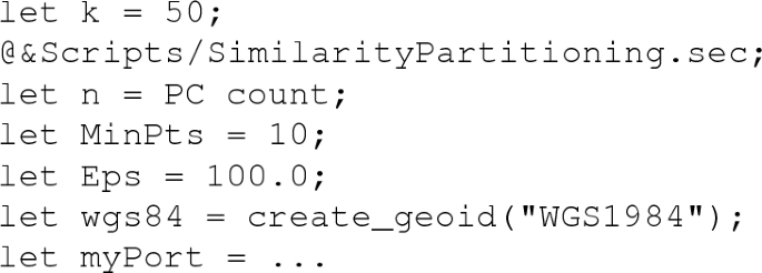
  The second line computes the set of partition centers PC, using SS and parameter k. The contents of the script SimilarityPartitioning.sec are shown in Sect. 6.6.

• 3. MW Share PC and some constant values with workers.

  

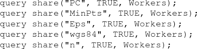
• 4. W Compute for each object s in $T_i$ its closest partition center $pc_j$ and the distance to it. Add to s attributes N and Dist representing the index j and the distance $d(s, pc_j)$. Further, compute for s all partition centers within distance $Dist + 2 \cdot Eps$ and add their indices in attribute N2. Repartition the resulting set of objects (tuples) by attribute N2, resulting in a distributed array V.

  

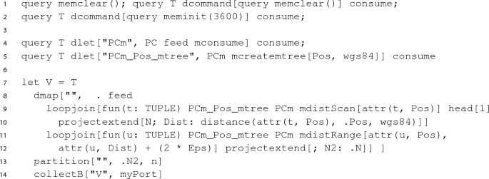
  In lines 1-2, main memory objects on the master and on the workers are deleted and for each worker, a bound of 3600 MB is set for main memory data objects. In lines 4-5, at each worker, the set PC is set up as a main memory relation together with an M-tree index over the Pos attribute. Using the wgs84 geoid, distances can be specified in meters, consistent with the definition of Eps. Note that the distributed array T is only used to specify the set of workers; its field values are not used.

  These data structures are used in the next step in lines 7-16. For each field of T, for each tuple t representing an element $s \in S$ the distance to the nearest partition center is computed (lines 10-11) and added to tuple t in attribute Dist; the index of the partition center is added in attribute N.

  Tuples are further processed in the next loopjoin, determining for each tuple the elements of PC within $Dist + 2 \cdot Eps$; the current tuple is joined with all these tuples, keeping only their index in attribute N2.

  Finally the resulting stream of tuples is repartitioned by attribute N2. Slot sizes are balanced across workers to achieve similar loads per worker in the next step.

• 5. W To each set $V_j$ apply a DBScan algorithm using parameters MinPts and Eps. Objects within subset $U_j$ (members) will be correctly classified as core objects and border objects; for the remaining objects in $V_j \setminus U_j$ (neighbors) we don’t care about their classification. Each object s from $V_j$ is extended by an attribute CID0 for the cluster number (-2 for noise) and a boolean attribute IsCore with value $|N_{Eps}(s)| \ge MinPts$. Cluster identifiers are transformed into globally unique identifiers by setting $CID = CID0 \cdot n + j$. The result is stored as $X_j$. The subset of $X_j$ containing the former members of $U_j$ is called $W_j$; $X_j \setminus W_j$ contains the neighbors of partition W.

  

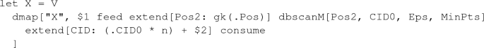
  The remaining problem is to merge clusters that extend beyond partition boundaries.

• 6. W For each $q \in (X_j \setminus W_j)$ retrieve $N_{Eps}(q) \cap W_j$. For each $p \in N_{Eps}(q) \cap W_j$, insert a tuple $(p, CID_p, IsCore_p,$ $N_p, q)$ into a set $Neighbors_j$.

  An equivalent formulation is:

  For each p in $W_j$ retrieve $N_{Eps}(p) \cap (X_j \setminus W_j)$. For each $q \in N_{Eps}(p) \cap (X_j \setminus W_j)$, insert a tuple $(p, CID_p, IsCore_p, N_p, q)$ into a set $Neighbors_j$.

  An advantage of the second formulation is that we need to search on the much smaller set $(X_j \setminus W_j)$ instead of $W_j$. As we will use a main memory index for this set, far less memory is needed and larger data sets can be handled.

  Redistribute Neighbors, once by the P and once by the Q attribute into distributed arrays NeighborsByP and NeighborsByQ, respectively, to prepare a join with predicate $P=Q$.

  

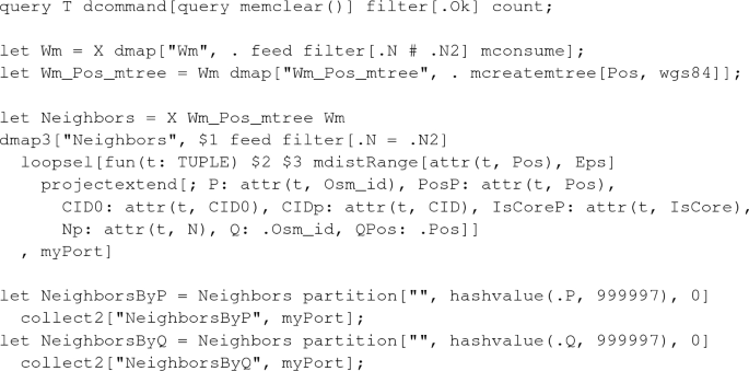
• 7. W For each pair of tuples $(q, CID_q, IsCore_q, N_q, p) \in NeighborsByQ,$

  $(p, CID_p, IsCore_p, N_p, q) \in NeighborsByP$:

  • (a) If both p and q are core objects, generate a task $(CID_p, CID_q)$ to merge clusters with these numbers; store tasks in a distributed table Merge

  • (b) If p is a core object, but q is not, generate a task $(q, N_q, CID_p)$ to assign to q the CID of p, since q is a boundary object of the cluster of p. Store such assignment tasks in a table Assignments.

  • (c) If p is not a core object, but q is, generate a task $(p, N_p, CID_q)$ to assign the CID of q to p.

  • (d) If neither p nor q are core objects, leave their cluster numbers unchanged.

  Redistribute assignments by the N attribute into distributed array Assignments.

  

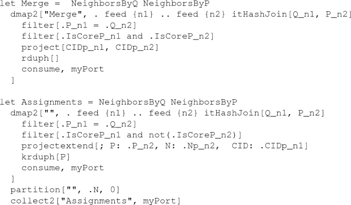
  For the Assignments, we remove duplicates with respect to only attribute P because we can assign the object p to only one cluster, even if it should be in the neighborhood of two different clusters.

• 8. MW Collect table Merge to the master into a graph MergeM. Further, set MaxCN on the master to the maximal component number over all $W_j$.

  

• 9. M Compute connected components in MergeM, adding to each node $CID_i$ a new component number, resulting in a pair $(CID_i, CIDnew_j)$. Collect pairs

  $(CID_i, CIDnew_j + MaxCN)$ in a table of renumberings Renumber.

  

• 10. MW Share Renumber with workers.

  

• 11. W For each partition $W_j$, apply the renumberings from $Assignments_j$ and those of Renumber to all elements. Now all objects in $W_j$ have received their correct cluster number.

  

6.6 Balanced partitioning

In Step 2 of the algorithm SimilarityClustering, partition centers are determined. Since in parallel processing each partition will be processed in a task by some worker, partition sizes should be as similar as possible. This is the easiest way to balance workloads between workers. As partition sizes are solely determined by the choice of partition centers, a good placement of partition centers is crucial.

To adapt to the density of the data set S to be clustered, there should be more partition centers in dense areas than in sparse areas. We therefore propose the following strategy: Compute for each element of S its radius r(s) as the distance to the k-th nearest neighbor, for some parameter k. We obtain for each $s \in S$ a disk with radius r(s). The disk will be small in dense areas, large in sparse areas. Place these disks in some arbitrary order but non-overlapping into the underlying space. That is, a disk can be placed if it does not intersect any disks already present; otherwise it is ignored.

The algorithm is shown in Fig. 11. In practice, it is not necessary to apply the algorithm to the entire data set to be clustered. Instead, a small random sample can be selected that reflects the density distribution. In our experiments, we use a sample of size 10000.

Fig. 11

Algorithm for computing partition centers

Figure 12 shows the result of the algorithm for the set of buildings in the German state of North-Rhine Westphalia. One can observe that small disks lie in the area of big cities.⁸

Fig. 12

Result of algorithm SimilarityPartitioning for buildings in the German state NRW

6.6.1 Implementation

An efficient implementation of this algorithm must rely on a data or index structure supporting k-nearest-neighbor search as well as distance range search. In Secondo, we can again use a main memory M-tree providing such operations.

In line 3, a main memory relation SSm is created from the sample SS. Next, a main memory M-tree index SSm_Pos_mtree indexing elements by Pos is built over SSm.

In lines 6-11, a main memory relation Balls is created where each tuple of SS is extended by an attribute Radius containing the distance to the kth-nearest neighbor. The distance is determined by an mdistScan operation which enumerates indexed tuples by increasing distance from the starting point, the position of the current tuple. The head operator stops requesting tuples from its predecessor after k elements; from its output via tail the last element is taken and the position value extracted.

In line 13 we determine the maximum radius of any element.

In lines 1-2, an empty main memory relation PCm is created with the same schema as that of Balls. Also an index $PCm\_Pos\_mtree$ is built over it, initially empty as well.

Lines 4-10 implement the second for each loop of algorithm SimilarityPartitioning. Each tuple from Balls is checked in the filter operator, using the condition that in a distance range search on the already present elements of PCm no tuples are found whose distance to this tuple is less than the sum of their radii. That is, their disks or balls would overlap. If no such tuple is found, the current tuple is inserted into PCm and the index over it.

Finally, from the main memory relation PCm a persistent relation PC with the partition centers is created, adding an index N, used in the main algorithm, and a circle for visualization.

7 Experimental evaluation

In this section we provide a brief experimental evaluation of the framework, addressing the quality of balanced partitioning, load balancing over workers, and speedup. A detailed evaluation of the clustering algorithm and comparison with competing approaches is left to future work.

7.1 Balanced partitioning

We consider the data set introduced in Sect. 6.5 of Buildings in the German state of NRW. There are 7842728 buildings. They are partitioned by the method of Sect. 6.6 yielding 123 partition centers as shown in Fig. 12. Each building is then assigned to its closest partition center (and possibly some more centers as explained in Step 4 of the algorithm). The total number of buildings assigned to slots is 8046065, so there are about 2.6 % duplicates assigned to several centers. The size distribution of the resulting partitions is shown in Fig. 13.

Fig. 13

Slot sizes for the partitioning of buildings in NRW (slots horizontal, slot size vertical)

One can see that slot sizes are somewhat balanced in the sense that there are no extremely large or small slots. Nevertheless they vary quite a bit. To describe this variation, we introduce a measure called utilization. The term utilization results from the idea that slots could be processed in parallel on different computers and the total time required is defined by the computer processing the largest slot. Utilization is the work done by all computers relative to what they could have done. Hence for a set of slot sizes $S = \{s_1, ..., s_n\}$, it is defined as $Util(S) = \frac{\sum _{i = 1, ..., n}s_i}{n \times \max _{i = 1, ..., n}s_i}$ which is the same as avg(S)/max(S).

For the slot sizes S shown in Fig. 13, we have $Util(S)=50.75\%$. Hence assigning these slots directly to different computers would not be very efficient.

7.2 Load balancing over workers

Fortunately in our framework slots are distributed over workers so that each worker processes several slots sequentially. By the standard “round robin” assignment of slots to workers, different slot sizes already balance out to some extent. The resulting worker loads are shown in Fig. 14. Here we have $Util( WL )=67.7\%$.

Fig. 14

Worker loads by round robin assignment for the partitioning of buildings in NRW

A still better load balancing between workers can be achieved by the collectB operator. It assigns partitions to workers based on their size (number of tuples) when they are transferred from a $\underline{\smash { dfmatrix }}$. The algebra definition does not prescribe by which algorithm this is done. In our implementation, the following heuristic is used:

• 1. Divide the set of available workers into standard and reserve workers (e.g., designate 5 % as reserve workers).

• 2. Sort slots descending by size into list S.

• 3. Traverse list S, assigning slots sequentially to standard workers. In each assignment, select a worker with the minimal load assigned so far.

• 4. Sort the worker loads descending by size into list A.

• 5. Traverse list A, removing from each assignment the last slot and assigning it to the reserve worker with the smallest assignment so far, until reserve worker loads get close to the average worker load (computed beforehand).

Here the basic strategy is to assign large slots first, small slots last to the worker with smallest load so far, which lets worker loads fill up equally. This happens in Steps 1 to 3. The last two steps 4 and 5 are motivated by the fact that sometimes in a relatively well balanced distribution there are a few workers with higher loads. The idea is to take away from them the last (small) assigned slots and move these to the reserve workers.

We have evaluated these strategies in a series of experiments on the given example database with Buildings in NRW. We vary the size of the sample SS using sizes 10000, 20000, and 50000; for each size the partitioning and assignment algorithm is run three times. The parameter k is fixed to 50. Note that with increasing sample size the number of partitions grows, because from each point a circle enclosing the closest k neighbors gets smaller. Hence more circles fit into the same space. Due to the randomness of samples, the numbers of partitions and all results vary a bit between experiments.

Table 1 shows the results. Here the last four columns have the following meaning:

UtilSizes	Utilization for the distribution of partition sizes as in Sect. 7.1
UtilRR	Utilization for worker loads with round robin assignment
UtilS	Utilization for worker loads with assignment descending by size (Steps 1 through 3 of the algorithm) without reserve workers
UtilSR	Utilization for worker loads with assigment descending by size and reassignment (Steps 1 through 5)

Table 1 Evaluation of Load Balancing Strategies

One can observe that we have about 3 slots per worker for sample size 10000 (as there are 40 workers), about 6 for 20000, and about 15 for 50000. The variation in slot sizes and the respective utilization (UtilSizes) remains at around 50% for the increasing number of partitions. However, the round robin utilization (UtilRR) improves from about 70% to about 85%.

Assignment descending by size (UtilS) is clearly better than round robin assignment and reaches already 95% for 6 slots per worker and 98% for 15 slots per worker. Using reserve workers and reassignment (UtilSR) can in some cases still improve utilization by a small percentage.

The fact that the partitioning algorithm returns slots of somewhat varying size is actually an advantage as having small slots allows one to fill up worker loads evenly. At the same time it is crucial not to have single slots that are extremely large.

In any case, by using enough slots per worker (e.g., 6 in this experiment) we can achieve an almost perfect load balancing in terms of the sizes of data to be processed.

7.3 Speedup

In this section we describe experiments with a larger data set to examine the speedup behaviour of the framework. Experiments are run on a small cluster consisting of 5 server computers, each with the following configuration:

• 8 cores, 32 GB main memory, 4 disks, Intel Xeon CPU E5-2630, running Ubuntu 18.04

• (up to) 8 workers, each using one core, 3.6 GB main memory, two workers sharing one disk

In addition, the master runs on one of the computers, using all memory, if needed. For the algorithm of this paper, the master uses almost no memory.

The data set to be clustered consists of the nodes of the OpenStreetMap data set for Germany. Each node defines a point in the plane; all geometries (e.g., roads, buildings, etc.) are defined in terms of nodes. There are 315.113.976 nodes. For clustering, we use the same parameters as in Sect. 6.5, namely $Eps=100$ meters, $MinPts=10$. In all experiments we use the same sample SS of size 30888 and parameter $k=100$ which leads to 188 partitions.

The algorithm of Sect.  6.5 was run 4 times, for sets of 10, 20, 30, and 40 workers denoted W10, ..., W40. W10 is considered as a baseline and we observe the speedup achieved relative to W10. Table 2 shows the elapsed time for the 11 steps of the algorithm.⁹

Table 2 Running Times for Similarity Clustering, 10 Workers

Due to the fact that the same precomputed sample was used in all 4 experiments, the computation of SS is missing in Step 1, which would add about 53 seconds. One can observe that Steps 1, 2, 3, 8, 9, 10 have negligible running times. Note that the global computation on the master in Steps 8 through 10 is in no way a bottleneck.

The remaining steps we consider in more detail for 10 to 40 workers in Table 3. Here within each step the running times for queries are given by the names of the resulting objects. The right part of the table shows the respective speedups defined as $time (W10)/ time (Wx)$. The numbers are visualized in Fig. 15.

Table 3 Running Times for Similarity Clustering

Especially Fig. 15a illustrates that by far most of the time is spent in the local DBScans (Step 5, X) and the initial partitioning of the data (Step 4, V). Regardless of running times, the right part of the table and Fig. 15a show the speedups for various queries. One can observe that computations involving shuffling of data have a weaker speedup (e.g., Step 6, $NeighborsBy ...$). This is because for more workers there is more data exchange. But for most queries good speedups can be achieved, e.g., by a factor around 3 going from 10 to 40 workers.

The overall running times and speedups are shown in Table 4.

Finally, Fig. 16 illustrates the result of the algorithm. The largest 3 clusters discovered have sizes of 158.798.786, 15.279.845, and 7.539.633, respectively. Fig. 16a shows the partition centers for Germany and two clusters at ranks 29 and 30 with 462.800 and 445.079 elements, respectively (of which only a few sample elements are selected for visualization). Figure 16b shows the bottommost cluster in more detail; the four local clusters that have been merged to the global cluster are illustrated by color. The boundaries of local clusters are defined by the Voronoi diagram over partition centers.

8 Conclusions

In this paper, we have proposed an algebra with formal semantics which allows a precise formulation of distributed algorithms or distributed query processing in general. It is based on the simple and intuitive concept of a distributed array, an array whose fields lie on and are processed by different computers. The algebra focuses on the aspect of distribution and is generic with respect to the possible field types or operations on them. It does, however, provide some specific operations to deal with collections of objects represented as relations. Otherwise, field types and operations are supplied by some single server database system, called the basic engine in this paper. Different such systems may be used in principle.

Fig. 15

a Running time, b Speedup, by Steps of the algorithm, for 10 to 40 workers

Table 4 Overall Running Times and Speedups

Fig. 16

a Partition centers for Germany and two clusters. b One cluster in detail, composed of four local clusters

It would not be satisfactory to present such an algebra without demonstrating its application to formulate distributed algorithms. Therefore, we have included a fairly advanced algorithm for distributed clustering. The algorithm is interesting in its own right: It includes a new technique for purely distance-based partitioning using any metric similarity function and it is the first precise distributed algorithm for density-based similarity clustering relying only on distance.

The formulation of the algorithm shows a new style of describing distributed algorithms. In addition to a precise mathematical formulation, it is possible to show the complete implementation in terms of high level operations of a database system with defined semantics, either of the distributed algebra or of the basic engine. One can see precisely which data structures and algorithms are used. This is in contrast to many published algorithms where certain steps are only vaguely described and hard to understand.

The framework has been implemented and is publicly available. In a brief experimental evaluation, we have studied the variation of partition sizes in the distance based partitioning, load balancing over workers, and speedup. The results show that partition sizes vary but are not extreme, and load balancing over workers can provide almost perfect load distribution, using a sufficient number of slots. Here it is crucial that the number of slots of a distributed array can be chosen independently from the number of workers. Finally, a good linear speedup is achieved for most queries.

Future work may address the following aspects:

• Provide fault tolerance for the distributed persistent database, for intermediate results in files, and for intermediate results in memory. For the persistent database and memory data, fault tolerance must maintain extensibility, that is, support arbitrary new indexes and other data types that are added to the basic engine.

• The presented algebra offers a basic generic layer for distributed query processing. On top of it more specialized layers may be added. This may include an algebra for distributed relations, providing several partitioning techniques and keeping track of partitioning in the data type, handling duplicates in spatial partitioning, and repartition automatically for joins. Another algebra may handle updates on distributed relations. All of this can be expressed in the Distributed Algebra, but will be easier to use at the higher level algebras.

• Provide an SQL level with cost-based optimization, handling of spatial partitioning in at least two and three dimensions (which includes moving objects) and spatial duplicate elimination.

• The given distributed arrays are static in their mapping of slots to workers. Provide dynamic distributed arrays which can adapt to a dataset whose density changes under updates, as well as to changing available resources.

• Embed other database systems such as PostgreSQL/PostGIS or MySQL in the role of basic engines.

Appendix

Operator and Syntax	Arguments	Result or Side Effect
s addcounter[Id, n]	s - a stream of tuples Id - a new attribute name n - an integer	Stream s extended by an integer attribute Id counting the tuples in the stream, starting from n
s addid	s - a stream of tuples	Stream s extended by an attribute TID containing the tuple identifier from the relation storing the tuple (normally contained only implicitly in the tuple representation). Via the TID value, a tuple can be accessed directly within its relation.
s t concat	s, t - two streams of tuples of the same type	The concatenation of the two streams
s consume	s - a stream of tuples	A relation containing the tuples from s
r count	r - a relation or stream of tuples	An integer containing the number of tuples of the relation or of the stream
s createmgraph2[a, b, f]	s - a stream of tuples a, b - two integer attributes of s f - a function from tuples in s into real	A main memory graph. The operator interprets each tuple t of the input stream s as a directed edge with source node identifier t.a and target node identifier t.b. Function f(t) determines the cost of the edge.
s dbscanM[a, Id, Eps, MinPts]	s - a stream of tuples a - an attribute of s Id - a new attribute name Eps - a real MinPts - an integer	A stream of tuples, containing all tuples from s. The operator has clustered tuples by attribute a using a dbscan algorithm with parameters Eps and MinPts, relying on a main memory M-tree built internally by the operator. The result of clustering is expressed by appending to each tuple a new integer attribute Id which contains cluster identifiers, or the value -2 for noise. In addition, a boolean attribute IsCore is added expressing whether the tuple represents a core or a border object.
i r exactmatch[p]	r - a main memory relation i - a B-tree index over r p - a value of the attribute type indexed in i	A stream of all tuples from t with value p in the indexed attribute.
s extend[$b_1: f_1, ..., b_k: f_k$]	s - a stream of tuples $b_1, ..., b_k$ - names for new attributes $f_1, ..., f_k$ - functions mapping a tuple from s into a value of some attribute type	A stream of tuples. Tuples t from s are extended by new attributes $b_1, ..., b_k$ with values $f_1(t), ..., f_k(t)$, respectively.
s extendstream[b : f]	s - a stream of tuples b - a name for a new attribute f - a function mapping a tuple from s into a stream of values of some attribute type	A stream of tuples. For each tuple $t \in s$ there are as many copies of t as there are values in f(t); each copy is extended by one of these values in attribute b.

Operator and Syntax	Arguments	Result or Side Effect
s extract[a]	s - a stream of tuples a - an attribute of s	The value of a of the first tuple in s
r feed	r - a relation	A stream of tuples from r
v feed	v - an atomic value of some attribute type	A stream of such values containing the single element v
s filter[f]	s - a stream of tuples f - a function from tuples of s into bool	A stream of tuples containing all tuples $t \in s$ for which $f(t) = true$
s head[n]	s - a stream of tuples n - an integer	A stream of tuples consisting of the first n tuples of s
s t itHashJoin[u, v]	s, t - two streams of tuples u, v - an attribute of s and an attribute of t of the same type	A stream of tuples representing the join of s and t with condition $s.u = t.v$. This is implemented via hashjoin.
s t itSpatialJoin[u, v]	s, t - two streams of tuples u, v - an attribute of s and an attribute of t of a spatial data type	A stream of tuples representing the join of s and t with the condition that the bounding boxes of u and v intersect. This is implemented via repeated search on a main memory R-tree.
s krduph[$a_1, ..., a_n, m$]	s - a stream of tuples $a_1, ..., a_n$ - attributes of tuples in s m - an integer (optional)	A stream of tuples from s. Keeps from each subset of tuples with equal values in attributes $a_1, ..., a_n$ only the first tuple. Implements duplicate elimination by hashing with optional parameter m as for rduph.
s loopjoin[f]	s - a stream of tuples f - a function, mapping a tuple t from s into a stream of tuples	A stream of tuples, where each input tuple $t \in s$ is concatenated with each tuple in f(t)
s loopsel[f]	s - a stream of tuples f - a function, mapping a tuple t from s into a stream of tuples	A stream of tuples, the concatenation of all tuple streams f(t) for $t \in s$
s max[a]	s - a stream of tuples a - an attribute of s	A value of the type of a representing the maximum over all tuples in s
s mconsume	s - a stream of tuples	A main memory relation containing the tuples from s
r mcreatemtree[a, g]	r - a main memory relation a - an attribute of r g - a geoid (optional)	A main memory M-tree index over r by attribute a. If a is of type $\underline{\smash { point }}$, a geoid argument can be given. In that case, distances are in meters.

Operator and Syntax	Arguments	Result or Side Effect
i r mdistRange[p, d]	r - a main memory relation i - an M-tree index over r p - a value of the attribute type indexed in i d - a real	a stream of tuples from r whose indexed attribute values lie within distance d from p.
i r mdistScan[p]	r - a main memory relation i - an M-tree index over r p - a value of the attribute type indexed in i	a stream of tuples from r ordered by increasing distance from p.
r mfeed	r - a main memory relation	a stream of tuples from r
g mg2connected-components	g - a main memory graph	a stream of tuples representing the edges of the graph. The operator computes strongly connected components and returns these in the form of an additional attribute CompNo appended to the tuples.
memclear()	none	Side effect: all main memory objects are deleted.
meminit(n)	n - an integer	Side effect: allow a total of n MB for main memory objects of this Secondo instance
s minsert[r]	s - a stream of tuples r - a main memory relation	Side effect: all tuples from s are inserted into r. Stream s is returned extended by a TID attribute, the tuple identifier allowing direct access to the tuple in the main memory relation.
s minsertmtree[t, a]	s - a stream of tuples containing a TID attribute t - a main memory M-tree a - an attribute of s	Side effect: all tuples from s are inserted into r by attribute a, using the TID to refer to the tuple position in the main memory relation. Stream s is returned.
s project[$a_1, ..., a_n$]	s - a stream of tuples $a_1, ..., a_n$ - attributes of tuples in s	A stream of tuples. Tuples from s are projected to attributes in $a_1, ..., a_n$.

Operator and Syntax	Arguments	Result or Side Effect
s projectextend [$a_1, ..., a_n$; $b_1: f_1, ..., b_k: f_k$]	s - a stream of tuples $a_1, ..., a_n$ - attributes of tuples in s $b_1, ..., b_k$ - names for new attributes $f_1, ..., f_k$ - functions mapping tuples from s into values of attribute types	A stream of tuples. Tuples t from s are projected to attributes in $a_1, ..., a_n$ and extended by new attributes $b_1, ..., b_k$ with values $f_1(t), ..., f_k(t)$, respectively.
s rduph[m]	s - a stream of tuples m - an integer (optional)	Stream s without duplicate tuples. The operator implements duplicate elimination by hashing. The optional parameter m defines the number of buckets, default is 999997.
s remove[$a_1, ..., a_n$]	s - a stream of tuples $a_1, ..., a_n$ - attributes of tuples in s	A stream of tuples. Tuples from s are projected to all attributes except $a_1, ..., a_n$.
s rename[x] s {x} (short notation)	s - a stream of tuples x - a string of letters and digits starting with a letter	stream s. However, all attributes have been renamed by appending string x
s some[n]	s - a stream of tuples n - an integer	A random sample from s of size n obtained by reservoir sampling
s sortby[$a_1, ..., a_n$]	s - a stream of tuples $a_1, ..., a_n$ - attributes of tuples in s.	stream s sorted lexicographically by the specified attributes.
s t symmjoin[f]	s, t - two streams of tuples f - a function with Boolean result relating a pair of tuples from s and t	A stream of tuples representing a general join of s and t with an arbitrary condition. This is implemented via a symmetric variant of nested-loop join.
s tail[n]	s - a stream of tuples n - an integer	A stream of tuples consisting of the last n tuples of s
s transformstream	s - a stream of tuples with a single attribute	A stream of the attribute values
s transformstream	s - a stream of values of some attribute type	A stream of tuples containing the values within an attribute Elem
s r updatedirect2 [TID; $a_1 : e_1 , ..., a_n : e_n$]	s - a stream of tuples r - a relation TID - an attribute in s containing tuple identifiers from r $a_1, ..., a_n$ - attributes of tuples in r $e_1, ..., e_n$ - functions mapping tuples from r into values of attribute types	A stream of tuples from r corresponding to the tuple identifiers within s. The tuple identifier and for each attribute, the old and the new value is contained in the tuple. (The output stream can be used to further update index structures on r.) Side effect: tuples in r are updated.

References

Alexander, A., Bergmann, R., Ewen, S., Freytag, J.C., Hueske, F., Heise, A., Kao, O., Leich, M., Leser, U., Markl, V., Naumann, F., Peters, M., Rheinländer, A., Sax, M.J., Schelter, S., Höger, M., Tzoumas, K., Warneke, D.: The Stratosphere platform for big data analytics. VLDB J 23(6), 939–964 (2014)
Alsubaiee, S., Altowim, Y., Altwaijry, H., Behm, A., Borkar, V., Bu, Y., Carey, M., Cetindil, I., Cheelangi, M., Faraaz, K., et al.: Asterixdb: a scalable, open source BDMS. Proc. VLDB Endow. 7(14), 1905–1916 (2014)
Baumann, P., Furtado, P., Ritsch, R., Widmann, N.: The Rasdaman approach to multidimensional database management. In: Proceedings of the 1997 ACM Symposium on Applied Computing, SAC ’97, pp. 166–173 (1997)
Buck, J.B., Watkins, N., LeFevre, J., Ioannidou, K., Maltzahn, C., Polyzotis, N., Brandt, S.A.: SciHadoop: array-based query processing in Hadoop. In: Scott Lathrop, Jim Costa, and William Kramer, editors, SC, pp. 66:1–66:11. ACM (2011)
Carbone, P., Katsifodimos, A., Ewen, S., Markl, V., Haridi, S., Tzoumas, K.: Apache \(\text{ flink}^{{\rm Tm}}\): stream and batch processing in a single engine. IEEE Data Eng. Bull. 38(4), 28–38 (2015)
Chang, F., Dean, J., Ghemawat, S., Hsieh, W.C., Wallach, D.A., Burrows, M., Chandra, T., Fikes, A., Gruber, R.E.: Bigtable: a distributed storage system for structured data. ACM Trans. Comput. Syst. 26(2), (2008)
Ciaccia, P., Patella, M., Zezula, P.: M-tree: An efficient access method for similarity search in metric spaces. In: VLDB’97, Proceedings of 23rd International Conference on Very Large Data Bases, pp. 426–435 (1997)
Website of the HashiCorp Consul project. https://www.hashicorp.com/blog/consul-announcement/, 2019. [Online; accessed 20-Dec-2019]
Dai, B., Lin, I.: Efficient map/reduce-based DBSCAN algorithm with optimized data partition. In: 2012 IEEE Fifth International Conference on Cloud Computing, pp. 59–66 (2012)
Dean, J., Ghemawat, S.: Mapreduce: Simplified data processing on large clusters. In: Proceedings of the 6th Symposium on Operating Systems Design and Implementation, OSDI’04, pp. 137–150. USENIX Association (2004)
DeCandia, G., Hastorun, D., Jampani, M., Kakulapati, G., Lakshman, A., Pilchin, A., Sivasubramanian, S., Vosshall, P., Vogels, W.: Dynamo: Amazon’s highly available key-value store. SIGOPS Oper. Syst. Rev. 41(6), 205–220 (2007)
Dong, W., Charikar, M., Li, K.: Efficient k-nearest neighbor graph construction for generic similarity measures. In: Proceedings of the 20th International Conference on World Wide Web, WWW 2011, pp. 577–586 (2011)
Eldawy, A., Mokbel, M.F.: Pigeon: a spatial mapreduce language. In: IEEE 30th International Conference on Data Engineering, ICDE 2014, pp. 1242–1245. IEEE Computer Society (2014)
Eltabakh, M.Y., Tian, Y., Özcan, F., Gemulla, R., Krettek, A., McPherson, J.: Cohadoop: flexible data placement and its exploitation in Hadoop. Proc. VLDB Endow. 4(9), 575–585 (2011)
Ester, M., Kriegel, H.-P., Sander, J., Xu, X.: A density-based algorithm for discovering clusters in large spatial databases with noise. In: Proceedings of the Second International Conference on Knowledge Discovery and Data Mining, KDD’96, pp. 226–231. AAAI Press (1996)
Website of the etcd project. https://etcd.io/, (2019). [Online; accessed 20-Dec-2019]
Fegaras, L.: A query processing framework for large-scale scientific data analysis, Transactions on Large-Scale Data- and Knowledge-Centered Systems, vol. 38, pp. 119–145 (2018)
Gates, A.F., Natkovich, O., Chopra, S., Kamath, P., Narayanamurthy, S.M., Olston, C., Reed, B., Srinivasan, S., Srivastava, U.: Building a high-level dataflow system on top of map-reduce: the Pig experience. Proc. VLDB Endow. 2(2), 1414–1425 (2009)
Geng, Y., Huang, X., Zhu, M., Ruan, H., Yang, G.: Scihive: Array-based query processing with HiveQL. In: TrustCom/ISPA/IUCC, pages 887–894. IEEE Computer Society (2013)
Website of GeoFabrik. https://download.geofabrik.de/, (2020). [Online; accessed 09-Jan-2020]
Ghemawat, S., Gobioff, H., Leung, S.T.: The Google File System. In: Proceedings of the Nineteenth ACM Symposium on Operating Systems Principles, SOSP ’03, pp. 29–43 (2003) ACM
Güting, R.H.: Second-order signature: a tool for specifying data models, query processing, and optimization. In: Proceedings of the 1993 ACM SIGMOD International Conference on Management of Data, pp. 277–286 (1993)
Güting, R.H., Behr, T.: Tutorial: distributed query processing in Secondo. http://dna.fernuni-hagen.de/Secondo.html/files/Documentation/General/DistributedQueryProcessinginSecondo.pdf (2019)
Güting, R.H., Behr, T., Düntgen, C.: Secondo: a platform for moving objects database research and for publishing and integrating research implementations. IEEE Data Eng. Bull. 33(2), 56–63 (2010)
Güting, R.H., de Almeida, V.T., Ansorge, D., Behr, T., Düntgen, C., Jandt, S., Spiekermann, M.: Secondo Programmer’s Guide. http://dna.fernuni-hagen.de/Secondo.html/files/Documentation/Programming/ProgrammersGuide.pdf, Version 10, September (2017)
Guttman, A.: R-trees: a dynamic index structure for spatial searching. SIGMOD Record 14(2), 47–57 (1984)
Website of Apache HBase. https://hbase.apache.org/, (2018). [Online; accessed 12-Feb-2018]
He, Y., Tan, H., Luo, W., Mao, H., Ma, D., Feng, S., Fan, J.: MR-DBSCAN: an efficient parallel density-based clustering algorithm using mapreduce. In: 17th IEEE International Conference on Parallel and Distributed Systems, ICPADS 2011, pp. 473–480 (2011)
Hunt, P., Konar, M., Junqueira, F.P., Reed, B.: Zookeeper: wait-free coordination for internet-scale systems. In: USENIX Annual Technical Conference. USENIX Association (2010)
Isard, M., Budiu, M., Yu, Y., Birrell, A., Fetterly, Dennis D.: Dryad: Distributed data-parallel programs from sequential building blocks. In: Proceedings of the 2nd ACM SIGOPS/EuroSys European Conference on Computer Systems 2007, EuroSys ’07, pp. 59–72 (2007)
Januzaj, E., Kriegel, H.P., Pfeifle, M.: DBDC: density based distributed clustering. In: Advances in Database Technology-EDBT 2004, 9th International Conference on Extending Database Technology, Heraklion, Crete, Greece, March 14-18, 2004, Proceedings, pp. 88–105 (2004)
Lakshman, A., Malik, P.: Cassandra: a decentralized structured storage system. SIGOPS Oper. Syst. Rev. 44(2), 35–40 (2010)
Lu, J., Güting, R.H.: Parallel Secondo: boosting database engines with Hadoop. In: 2013 International Conference on Parallel and Distributed Systems, 738–743, 2012
Lulli, A., Dell’Amico, M., Michiardi, P., Ricci, L.: NG-DBSCAN: scalable density-based clustering for arbitrary data. PVLDB 10(3), 157–168 (2016)
Malewicz, G., Austern, M.H., Bik, A.J.C., Dehnert, J.C., Horn, I., Leiser, N., Czajkowski, G.: Pregel: a system for large-scale graph processing. In: Proceedings of the ACM SIGMOD International Conference on Management of Data, SIGMOD 2010, pp. 135–146 (2010)
McKinney, W.: Data structures for statistical computing in python. In Proceedings of the 9th Python in Science Conference, pp. 51–56 (2010)
MRQL. The Apache MRQL Project (2019). http://incubator.apache.org/projects/mrql.html - [Online; accessed 20-Dec-2019]
Nidzwetzki, J.K., Güting, R.H.: Distributed Secondo: an extensible and scalable database management system. Distribut. Parall. Databases 35(3–4), 197–248 (2017)
T.E. Oliphant. A guide to NumPy, volume 1. Trelgol Publishing USA (2006)
Olston, C., Reed, B., Srivastava, U., Kumar, R., Tomkins, A.: Pig Latin: A not-so-foreign language for data processing. In: Proceedings of the 2008 ACM SIGMOD International Conference on Management of Data, SIGMOD ’08, pp. 1099–1110 (2008)
O’Neil, P., Cheng, E., Gawlick, D., O’Neil, E.: The log-structured merge-tree (LSM-tree). Acta Inf. 33(4), 351–385 (1996)
Oracle. The Documentation of the spatial GeoRaster feature, (2019) https://docs.oracle.com/cd/B19306_01/appdev.102/b14254/geor_intro.htm. Accessed 20 Dec 2019
Patwary, M.M.A., Palsetia, D., Agrawal, A., Liao, W., Manne, F., Choudhary, A.N.: A new scalable parallel DBSCAN algorithm using the disjoint-set data structure. In: SC Conference on High Performance Computing Networking, Storage and Analysis, SC ’12, Salt Lake City, November 11-15, 2012, p 62 (2012)
PostGIS. The Documentation of the raster datatype, (2019). https://postgis.net/docs/RT_reference.html . Accessed 20 Dec 2019
Shvachko, K., Kuang, H., Radia, S., Chansler, R.: The Hadoop distributed file system. In: Proceedings of the 2010 IEEE 26th Symposium on Mass Storage Systems and Technologies (MSST), MSST ’10, pp. 1–10. IEEE Computer Society (2010)
Sinthong, P., Carey, M.J.: AFrame: extending dataframes for large-scale modern data analysis (Extended Version). CoRR, (2019). arXiv:1908.06719
Stonebraker, M., Brown, P., Becla, J., Zhang, D.: SciDB: a database management system for applications with complex analytics. Comput. Sci. Engg. 15(3), 54–62 (2013)
The Open Street Map Project. Open Street Map Project Website, (2019). http://www.openstreetmap.org. Accessed 20 Dec 2019
The Website of the RocksDB Project. Website of the RocksDB Project, (2019). http://rocksdb.org/. Accessed 20 Dec 2019
Thusoo, A., Sarma, J.S., Jain, N., Shao, Z., Chakka, P., Anthony, S., Liu, H., Wyckoff, P., Murthy, R.: Hive: a warehousing solution over a map-reduce framework. Proc. VLDB Endow. 2(2), 1626–1629 (2009)
Valdés, F., Behr, T., Güting, R.H.: Parallel trajectory management in Secondo. Technical report, Fernuniversität in Hagen, Informatik-Report 380 (2020)
Xin, R.S., Gonzalez, J.E., Franklin, M.J., Stoica, I.: GraphX: a resilient distributed graph system on Spark. In: First International Workshop on Graph Data Management Experiences and Systems, GRADES 2013, co-loated with SIGMOD/PODS 2013, New York June 24, 2013, p. 2 (2013)
Xu, X., Jäger, J., Kriegel, H.P.: A fast parallel clustering algorithm for large spatial databases. Data Min. Knowl. Discov. 3(3), 263–290 (1999)
Website of the Apache Hadoop YARN (Yet Another Resource Negotiator) project. https://hadoop.apache.org/docs/current/hadoop-yarn/hadoop-yarn-site/YARN.html, (2019). Accessed 20 Dec 2019
Yu, Y., Isard, M., Fetterly, D., Budiu, M., Erlingsson, U., Gunda, P.K., Currey, J.: DryadLINQ: A system for general-purpose distributed data-parallel computing using a high-level language. In: 8th USENIX Symposium on Operating Systems Design and Implementation, OSDI 2008, pp. 1–14 (2008)
Zaharia, M., Chowdhury, M., Das, T., Dave, A., Ma, J., McCauly, M., Franklin, M.J., Shenker, S., Stoica, I.: Resilient distributed datasets: A fault-tolerant abstraction for in-memory cluster computing. In: Proceedings of the 9th USENIX Symposium on Networked Systems Design and Implementation, NSDI 2012, pp. 15–28 (2012)
Zaharia, M., Xin, R.S., Wendell, P., Das, T., Armbrust, M., Dave, A., Meng, X., Rosen, J., Venkataraman, S., Franklin, M.J., Ghodsi, A., Gonzalez, J., Shenker, A., Stoica, I.: Apache Spark: a unified engine for big data processing. Commun. ACM 59(11), 56–65 (2016)
Zhang, Y., Kersten, M., Manegold, S.: SciQL: Array Data Processing Inside an RDBMS. In: Proceedings of the 2013 ACM SIGMOD International Conference on Management of Data, SIGMOD ’13, pp. 1049–1052 (2013)
Funding
Open Access funding enabled and organized by Projekt DEAL.
Author information
Authors and Affiliations
Corresponding author
Additional information
Publisher's Note
Springer Nature remains neutral with regard to jurisdictional claims in published maps and institutional affiliations.