
Empirical Insights from a Study on Outlier Preserving Value Generalization in Animated Choropleth Maps


1
Interfaculty Department of Geoinformatics-ZGIS, University of Salzburg, 5020 Salzburg, Austria
2
AMAG Austria Metall AG, 5282 Ranshofen, Austria
*
Author to whom correspondence should be addressed.
ISPRS Int. J. Geo-Inf. 2021, 10(4), 208; https://doi.org/10.3390/ijgi10040208
Submission received: 11 February 2021
/
Revised: 15 March 2021
/
Accepted: 16 March 2021
/
Published: 1 April 2021
(This article belongs to the Special Issue Multimedia Cartography)
Abstract
:Time series animation of choropleth maps easily exceeds our perceptual limits. In this empirical research, we investigate the effect of local outlier preserving value generalization of animated choropleth maps on the ability to detect general trends and local deviations thereof. Comparing generalization in space, in time, and in a combination of both dimensions, value smoothing based on a first order spatial neighborhood facilitated the detection of local outliers best, followed by the spatiotemporal and temporal generalization variants. We did not find any evidence that value generalization helps in detecting global trends.
1. Introduction
Temporal animation of choropleth maps is a popular way to depict time-series data aggregated to enumeration units. Although movies from snapshots of choropleth maps are simple to understand conceptually, they often exceed our perceptual limits [1].
When viewing the sequence of time slices, users can easily miss important changes in the map during a saccade [2] or due to weak change signals from unattended areas of peripheral vision [3,4]. However, even when people apparently sense the often simultaneous changes in the quick succession of maps, they are easily overwhelmed by the sheer amount of transient information and often fail to derive appropriate mental models of the mapped process [1]. According to cognitive load theory [5,6], the cognitive bottleneck is the visual working memory, not able to store more than four new objects simultaneously [7]. Visual information, like objects changing their color in the map, needs to be shuttled into long-term memory to understand and further build upon it. If new information arrives during this process, the exchange between working memory and long-term memory is either cancelled by switching attention to new visual objects (“proactive inhibition”), or the new objects cannot be perceived due to blocked working memory resources by prior objects (“retroactive inhibition”) [1]. The resulting “cognitive overflow” is further exacerbated in situations of split attention, when, for example, the user tries to simultaneously grasp the changing map contents and its (temporal) legend [8].
1.1. Solutions Proposed to Reduce Cognitive Load
Cartographers explored a number of ways to reduce cognitive load and make animations more accessible. While many ideas are related to the user interface design with the implicit or explicit goal to minimize split attention and/or maximize user control [9,10,11,12,13,14], others focus on the transition between time-steps [15,16], on techniques to highlight important changes [17], or on the relation between data complexity and animation speed. Multimäki and Ahonen-Rainio [18] equalize the temporal scale according to the temporal density of change, slowing down the animation in busy times, while increasing animation pace when the number of changes is low. Although this seems useful to limit cognitive load, it presumably fails to convey the temporal structure in the development of spatial processes. Moreover, stretching time to limit the amount of change between two subsequent frames requires adequate data. In case of low temporal sampling frequency, the amount of change between two adjacent time-steps/frames might already exceed cognitive limits, regardless of the slow animation pace. Thus, in addition to appropriate user interfaces, approaches are needed that reduce cognitive load by reducing the visual complexity of the data itself by means of generalization.
In order to remove “flicker” in choropleth map animations resulting from spurious value-changes over time, Monmonier [19] developed a classification algorithm trying to optimize class breaks in this respect. As it turned out that the problem could not be solved sufficiently by (crisp) data classification, he advocated for temporal averaging instead, and hypothesized on the usefulness of kernels that simultaneously smooth the data in the spatial and the temporal dimension [20]. Harrower [21] highlighted the benefits of spatial and temporal aggregation to facilitate change detection in a temporal animation of remotely sensed data. Giving general advice for effective animated map design, Harrower [10] advocated for highly generalized animated maps by using data filtering, data smoothing, or aggregating data into two or three classes. Even though he later withdrew his statement on the use of classification [22], he re-emphasized that filtering and smoothing is an important design principle of animated maps to provide a coherent “big picture” [9].
1.2. Research Gap
To the best of our knowledge, there was only a single empirical study addressing generalization in animated choropleth maps so far: McCabe [23] investigated the effects of temporal aggregation and temporal smoothing on two tasks (picking the map frame with the overall highest values, comparing the cumulative values between two regions over the whole animation) related to the interpretation of measles epidemics data in Niger. For both tasks, he could not find benefits from temporal averaging of data, but rather found a non-significant tendency that participants who used temporally smoothed data even performed worse in picking the “maximum” map frame, which is understandable due to the smoothing of instantaneous peaks. Given the notion that animated choropleth maps are most useful to gain an overview of the development of spatial process [22,24,25] and significant local outliers (polygons with values greatly differing from their neighbors in space and time) thereof [26], it is questionable whether the tasks in McCabe’s experiment were the best choice to tackle potential benefits of animated choropleth maps generalization. To fill this gap, we conducted an experiment to evaluate the effect of local outlier preserving value generalization in space, in time, and in a combination of both dimensions on the detection of overall trends and local outliers in animated choropleth maps.
1.3. Document Organization
In the following section, we illustrate the design of our experiment and characterize the group of 440 test-persons who participated in our study. Then, we present the analysis of the obtained data, while adding insights from an extensive pilot study and thoroughly discuss our results in the light of perception and cognition of animated maps. We conclude with an outlook on future research opportunities.
2. Methods
To find out if and how different forms of value generalization of unclassed choropleth map animations affect the ability of users to detect general trends and local outliers thereof, we developed the following online-experiment: Participants saw short, synthetic map animations, each consisting of a general trend and two local outliers in space and time. Immediately after each animation ended, it was replaced by a set of six outlier candidates (first part of the experiment) or three trend candidates (second part of the experiment). From these sets participants had to select correct outliers and the correct trend, respectively. Having used differently generalized versions of the presented animations (non-generalized reference, temporal-, spatial-, and spatiotemporally generalized versions), we were able to examine the effect of generalization mode on the ability of users to correctly detect local outliers and overall trends.
2.1. Animated Map Stimuli
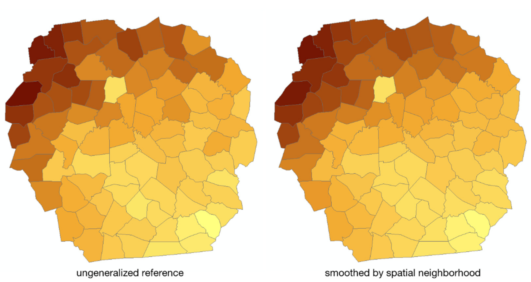
Each animation stimulus shows a map of 85 irregular but similar sized polygons that consists of 14 map frames. It was displayed at the size of 512 × 512 px and at the speed of five frames per second. Polygon values were simulated in GAMA (https://gama-platform.github.io) using a model that produces moving clusters embedded in a global trend and randomly adds local outliers to the otherwise highly autocorrelated data in space and time. From a large number of simulation results, we chose for the final map-stimuli those that contained exactly two local outlier polygons in space and time. Local outliers were determined by a heuristic that evaluates the value-difference of polygons to their first order space-time neighborhood, while considering the global autocorrelation of the data (see Traun and Mayrhofer [26] for further details). Spatiotemporal autocorrelation of all stimuli is rather similar with Moran’s Is [27] between 0.84 and 0.93. From these reference stimuli, we derived three differently generalized versions by smoothing polygon values by their first order spatial, spatiotemporal, or temporal neighbors, respectively, while excluding the two local outlier-polygons from the generalization process. For data smoothing, we used the methods and software provided by Traun and Mayrhofer [26] and applied a CIE Lab-interpolation based, sequential yellow-to-brown color scheme to the unclassed data, using a linear min-max stretch (Figure 1).
2.2. Response Items
After having seen a stimulus, participants had to choose the correct local outliers (first part of the experiment) and the appropriate global trend (second part) from a set of outlier and trend candidates, respectively.
2.2.1. Outlier Response Items
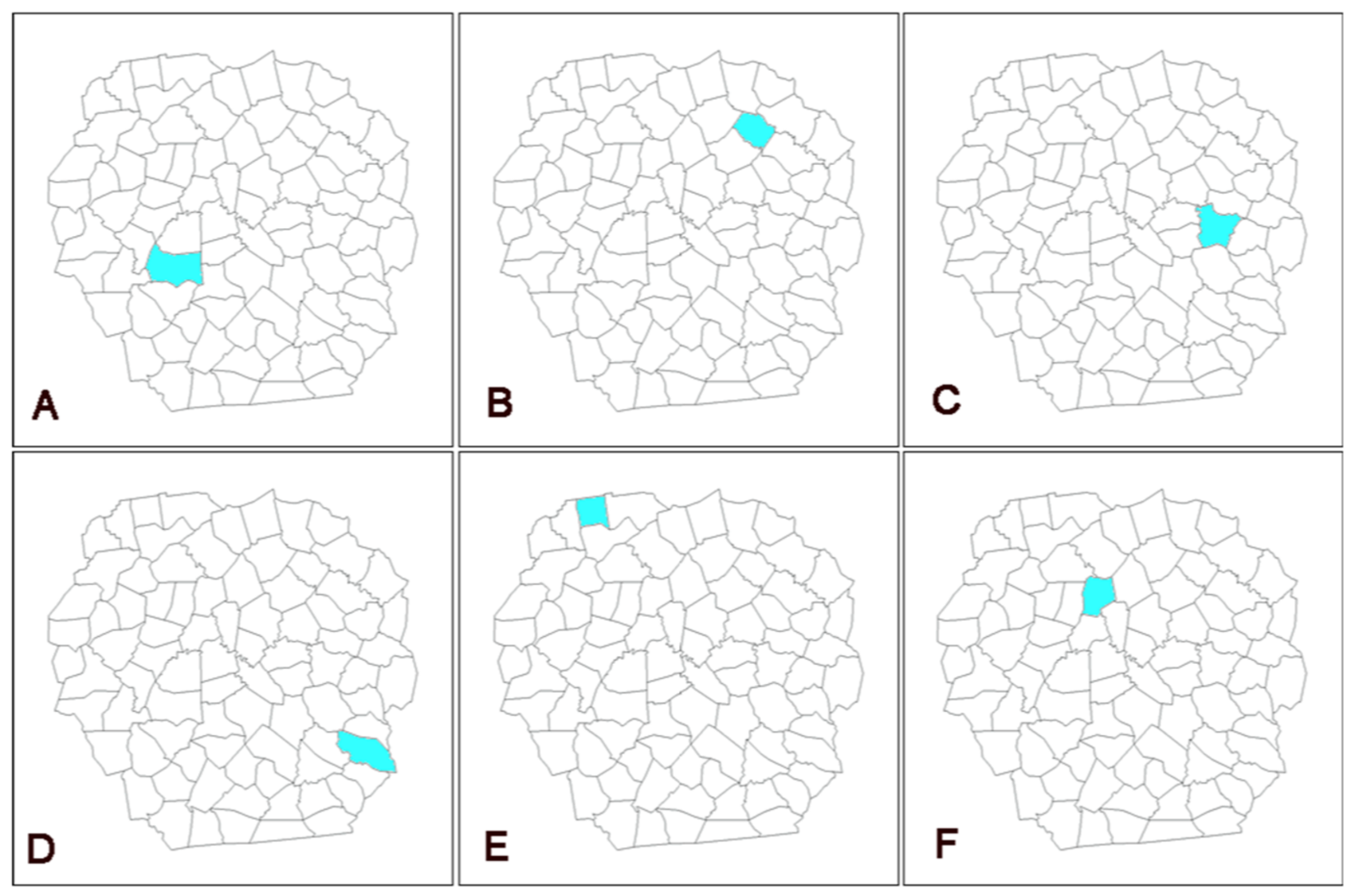
Six basemaps, highlighting one outlier candidate each, contain the two correct outliers from the stimulus and four wrong outlier candidates (Figure 2).
Contrary to the correct outlier candidates, wrong outlier candidates have a low value difference to their spatiotemporal neighborhood throughout the whole animation. Together with a dispersed distribution of outlier candidates over the basemap, this should prevent misinterpretation of non-outlier polygons as local outliers.
2.2.2. Trend Response Items
Global trend response items were produced by downscaling animated map stimuli to 160 × 160 px and applying a 15 px blur filter (Figure 3). To prevent participants from identifying trend response items not by the trend, but from the position of local outliers, they were replaced with the mean value/color of their neighbors before applying the filter. While correct global trend response items were produced from the respective stimulus animations, two alternative (wrong) items per response item set were derived from other stimuli or unused stimulus candidates. Each response item is started with a mouse click and could be replayed as often as desired. Response items are available together with other data from this research at https://tinyurl.com/mapstudyresults, as indicated in the data availability statement at the end of this document.
2.3. Study Design and Implementation
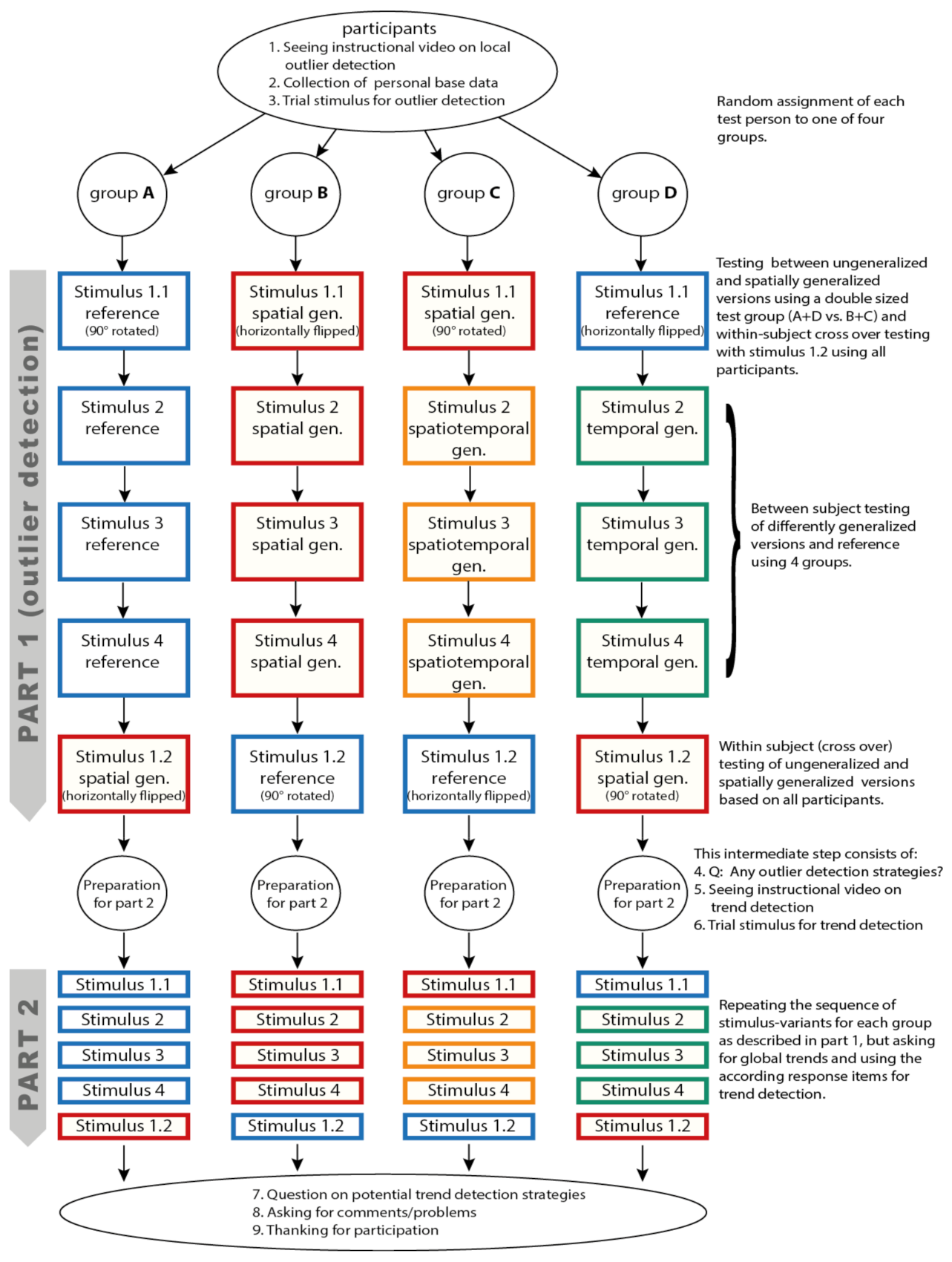
We decided for a mixed study design, which is based on four-group between subject-design, according to the modes of generalization (A-ungeneralized reference, B-spatial generalization, C-spatiotemporal generalization, and D-temporal generalization—refer to Stimulus 2, 3, and 4 in Figure 4).
From the results of a pilot study, we assumed that spatial generalization might have the highest impact on perception. Thus we developed a backup strategy for low participation numbers and small effect sizes and complemented the four-group design for Stimulus 2, 3, and 4 by a (double sized) two group between-subject plus a within-subject design for Stimulus 1. While Stimulus 1 was limited to two modes (ungeneralized and spatially generalized version), every participant saw the ungeneralized reference and the spatially generalized version of this stimulus in both parts of the experiment (refer to Stimulus 1.1 and 1.2 in Figure 4).
The experiment was set up as an online-study. Participation was restricted to desktop operating systems to prevent the use of small displays. Stimulus preloading ensured uninterrupted playback in case of low internet bandwidth.
Having accepted the invitation, participants saw a video, explaining the task of looking for two local outliers in an exemplary stimulus animation and demonstrating the selection of response items. Then, data on variables controlling for age, sex, visual impairments, map use experience, computer gaming frequency, and highest educational level were collected. Before participants went through the first set of stimulus sequences, they practiced outlier detection with a trial stimulus. Then, they were randomly assigned to one of four groups (Figure 4). Each stimulus sequence includes three steps:
- 3-second countdown and automatic start of the animation.
- Immediate replacement of the animation with response items for local outliers to choose from (Figure 2).
- Rating of the difficulty of the task.
After finishing this first part, participants were asked to comment on potential strategies to identify and remember outliers. Then, they saw an instructional video on trend detection and practiced again with a trial stimulus, before entering the second part of the experiment. There, each group saw exactly the same stimuli-variants from the first part, but had to choose the correct trend response item out of three options (Figure 3). Finally, participants reported on trend detection strategies and were asked for feedback on the overall survey and any (technical) issues they encountered.
2.4. Participants and Data
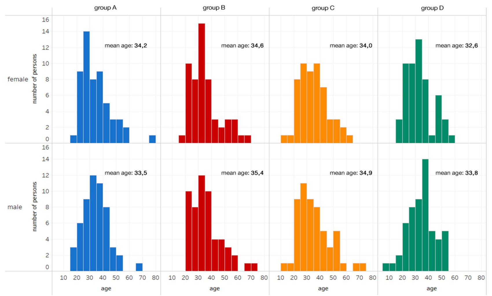
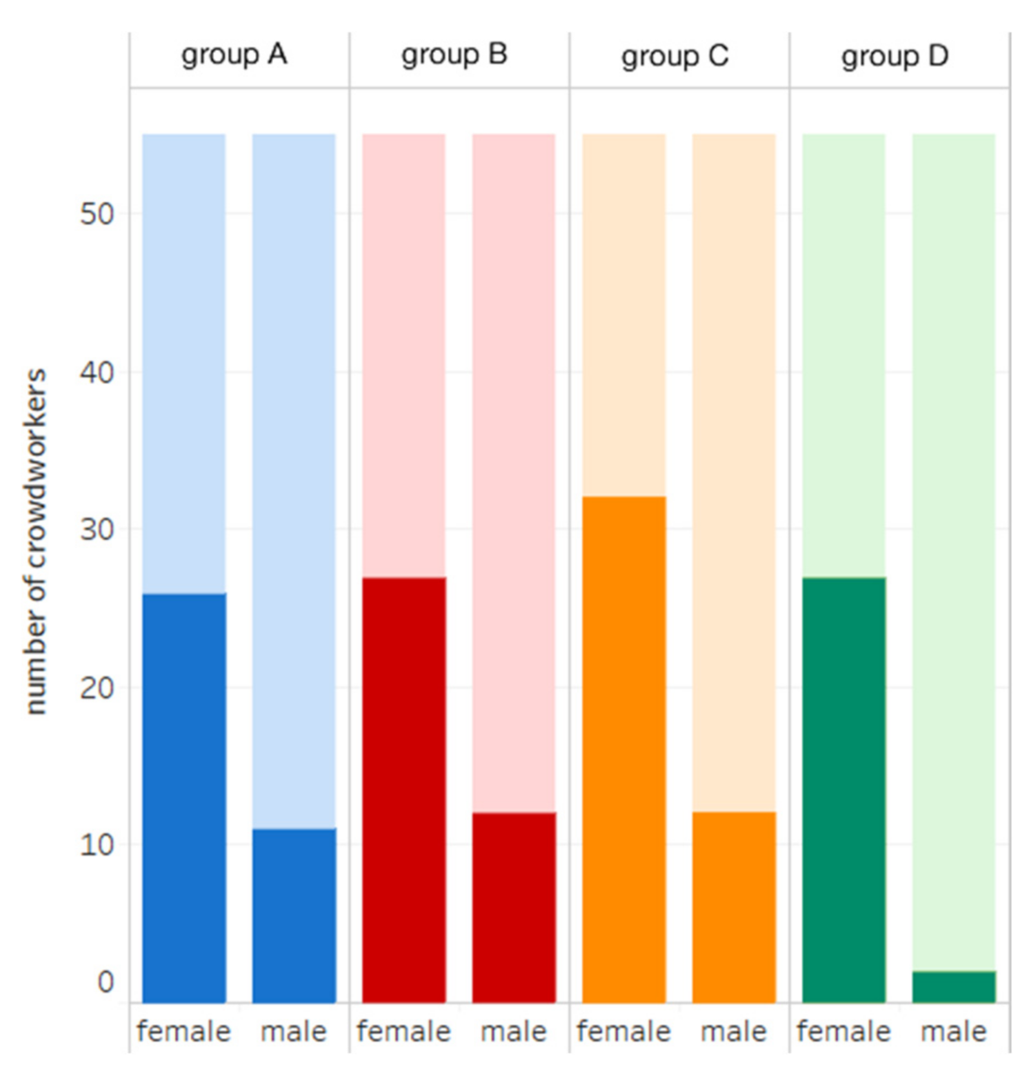
The main study took place in December 2020. Invitations were distributed via social media and sent out by email to geography students and students/recent graduates from a distance learning program in GIS with the request for further dissemination. This effort resulted in 308 complete datasets with slightly different group sizes, different age distributions, and remarkably more male participants. To be more balanced in these aspects and considering positive experiences in the use of online crowdsourcing services in cognitive experiments [28] we complemented data with crowdworker-responses. By using stratified sampling in respect to age and sex, we acquired 169 crowdworkers at the platform clickworker.de. Each of them was compensated with 1.10 Euro for their time investment (median: 9 min). From the combined set of 477 responses, we randomly removed three male responses from group B and two male responses from group C to have equally sized groups. Referring to Crump et al. [28], we got rid of sloppy attempts by calculating a quality index (watching the videos to end, time used for provision of personal data and comments, overall outlier and trend detection performance) and removed the worst four male and female attempts from each group. The final dataset comprises four equally sized groups, each consisting of 55 male and 55 female responses. For age distributions and the share of crowdworkers per group see Figure 5 and Figure 6. The distribution of cartographic competences among the participants is given in Table 1.
To analyze whether or not people prefer generalized map animations, the main study was supplemented by data from our extensive pilot study, which was also conducted in an online-format. There, 334 (different) persons saw an infinitely looped, successive comparison (A = Reference, B = spatially generalized version) of Stimulus 4 and were asked to verbally describe differences and issue preferences.
3. Results
Statistical analysis was done in R [29], predominantly using the package npmv [30]. It compares the multivariate distributions for a single explanatory variable (like generalization mode) using nonparametric techniques and is even suitable for small samples. Using approximations for ANOVA Type, Wilks′ Lambda, Lawley Hotelling, and Bartlett Nanda Pillai Test statistics along with according permutation tests, the package allows us to compare the results of up to eight statistical testing approaches, whereas the actual number of applicable tests depends on the data structure [30]. With one exception, we received good agreement between different tests, which is an indication for the stability of the obtained p-values. As advised by Ellis, Burchett, Harrar, and Bathke [30], and for sake of readability, the p-values for Wilks′ Lambda are reported whenever this test was applicable. In all other cases, we provide the p-values from the ANOVA Type test. Reported p-values were Bonferroni-corrected for multiple testing.
3.1. Local Outlier Detection
For each person and stimulus instance, the numbers of correctly detected local outliers (0–2) and wrongly indicated outliers (up to 4 “false positives” possible) were recorded.
3.1.1. Correctly Detected Local Outliers
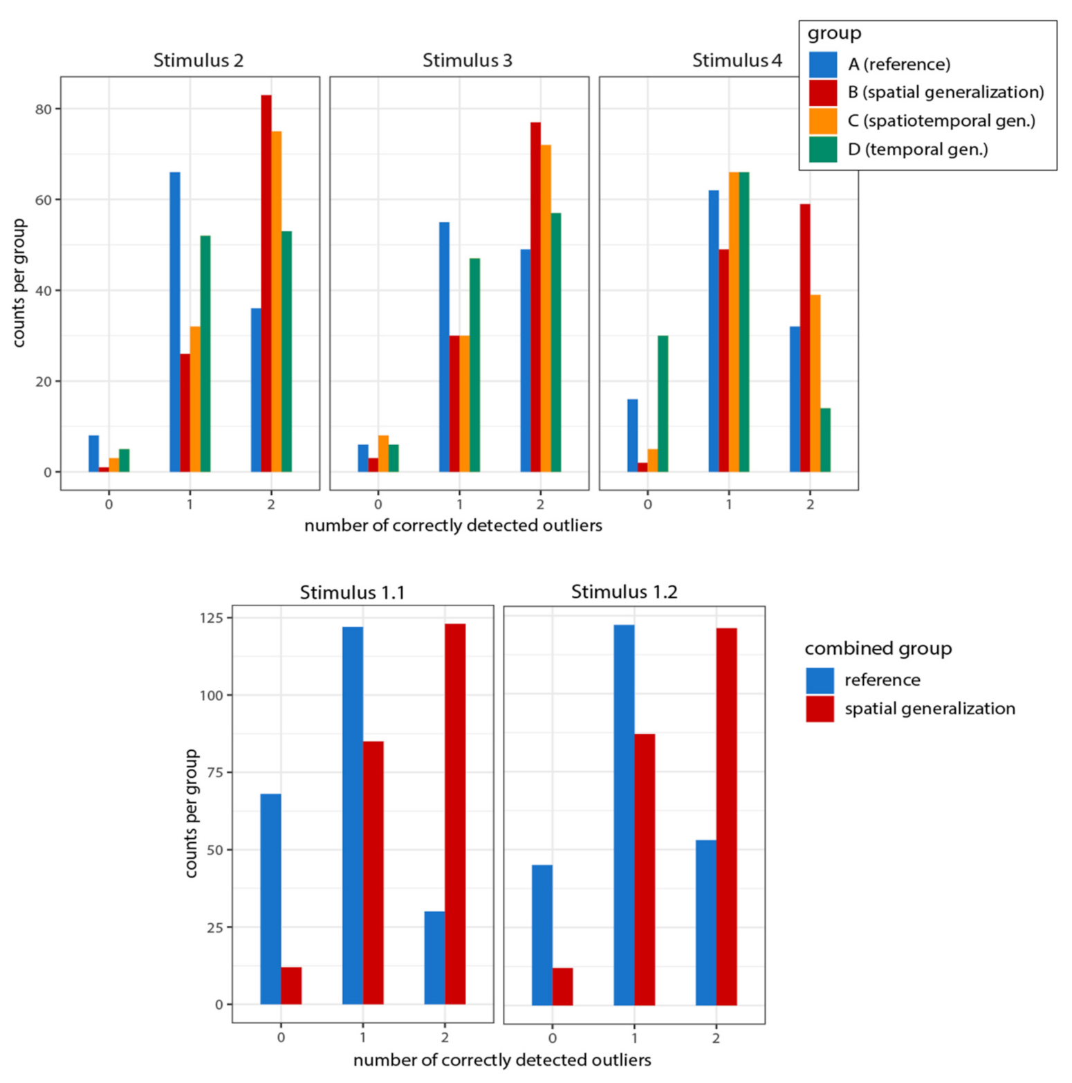
To see the influence of the independent variable “generalization mode” on the ability to correctly detect local outliers, we summed up the absolute counts per group (A,B,C,D) for 0, 1, and 2 correct outliers for each of the stimuli 2, 3, and 4. For stimulus 1.1 and 1.2, we combined the groups A + D and B + C as shown in Figure 4 and calculated the frequencies of 0, 1, and 2 correct outliers accordingly. The resulting pattern (Figure 7) clearly shows that (outlier preserving) generalization using the direct neighbors in space facilitated the detection of both local outliers best, followed by spatiotemporal and temporal generalization variants.
People having seen generalized stimuli outperformed respondents from the reference group in all but one instance: For Stimulus 4, the temporally smoothed variant led to the poorest results. We, however, do not attribute any particular meaning to this, as we had tested exactly these two variants (reference and temporally generalized version) of stimulus 4 in our pilot study. Results showed quite similar outlier detection performance for both groups consisting of 84 and 82 (different) persons, respectively. Therefore, we consider this inconsistency in the main experiment to be a statistical outlier.
Global statistical testing (combined for stimuli 2, 3, and 4) for each of the 3 generalization variants against the reference group rejected the null hypothesis (no difference) on the α = 0.01 level (p < 0.001). When, however, testing the temporal variant against the reference just for Stimulus 2 and 3 while excluding the erratic result from Stimulus 4, the (Bonferroni corrected) result is not significant anymore (p = 0.22). Thus, an effect of outlier preserving, temporal generalization on outlier detection seems questionable.
Statistical analysis of the double sized group results from stimulus 1.1 and 1.2 confirms the highly significant effect of outlier preserving smoothing in space on local outlier detection (p < 0.001). The relatively improved performance of the reference group in Stimulus 1.2 probably results from evolving strategies for local outlier detection when being exposed to this (last) stimulus. An additional within-person crossover test based on stimulus 1 further confirms the outcome from the between group tests: For each person, the number of correctly detected outliers from the generalized version was subtracted from the according number from the ungeneralized reference stimulus. For the resulting distribution the 95%-bootstrap-confidence interval for the mean is given by [−0.640, −0.493] and the null hypothesis (mean is equal to 0) is rejected.
3.1.2. False Positive Outliers
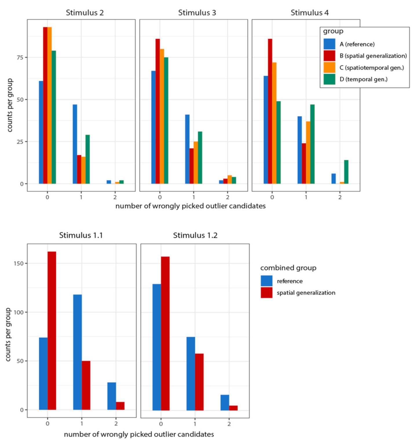
As test persons were informed of the presence of two local outliers in each animation, the theoretical possibility of three or four wrong picks did not happen. In most cases, zero or one wrong candidates were chosen (Figure 8). Although results are not reciprocal to correct outlier identification, they follow similar, yet inverted (less is “better” in this case) lines.
Differences between the reference group and the spatial and spatiotemporal groups are highly significant (p < 0.001), with both groups constantly outperforming the reference group. Again, the temporal group performed worse than the reference group for Stimulus 4. Including this Stimulus in the statistical analysis leads to inhomogeneous p-values in the applied tests, ranging from p = 0.008 (Wilks′ Lambda) to p = 0.04 (ANOVA Type permutation test). Limiting the test to Stimulus 2 and 3 results in an insignificant p-value of 0.08 (Wilks′ Lambda).
A test of the double-sized groups in Stimulus 1.1 and 1.2 confirms the differences between reference and spatial generalized variants (both p < 0.001). Again, a general learning effect might be the reason for the improved results of the reference group in the second (flipped and rotated) instance of this stimulus.
3.2. Global Trend
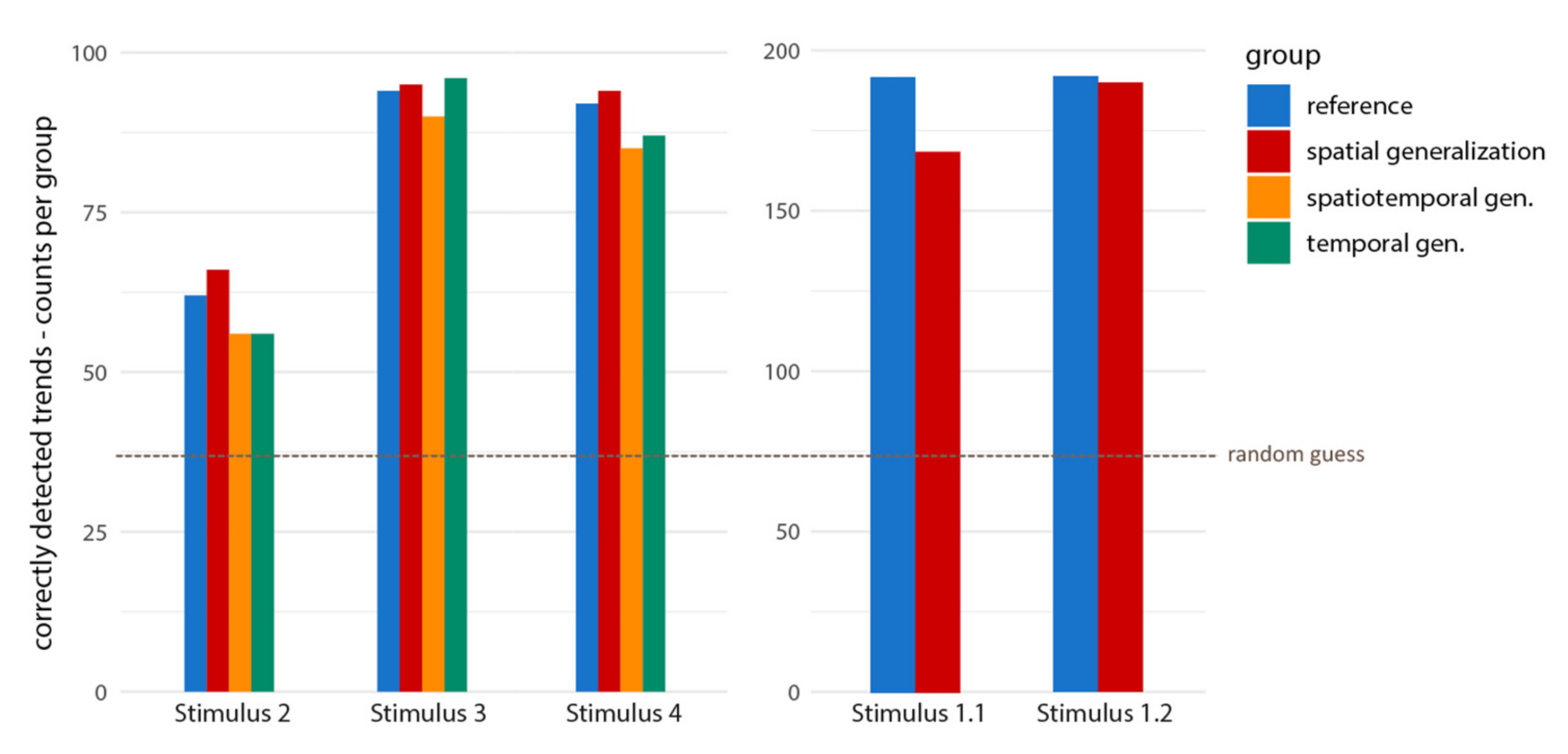
We started our empirical studies with the assumption, that value generalization removing “visual noise” from choropleth map animations will facilitate the detection of the remaining overall trends. According to our quantitative results (Figure 9), this is not the case.
Although there are seemingly small benefits for the spatial generalization variant for Stimulus 2, 3, and 4, group differences are not significant. Interestingly, there is a highly significant result (p = 0.005) pointing to the opposite direction for Stimulus 1.1. As this was the first stimulus participants were exposed to in the second part of the survey (after one trial stimulus for practicing), several persons from the spatial group probably were distracted from their trend detection task by the quite salient outliers in this instance and involuntarily turned their attention back to “outlier detection mode”. The nearly equal performance of both groups for the (identical) last stimulus of the survey (Stimulus 1.2) and some self-observation when going through the survey support this interpretation.
3.3. Person-Related Covariates
Due to the large number of participants and their random assignment to groups, potentially confounding variables like cartographic competence or educational level are distributed quite evenly among groups. To test the influence of those variables on outlier detection capabilities, we derived a personal outlier score for each participant by adding up all correctly detected outliers for the five stimuli seen. In the same manner, a personal trend score (sum of correct trends) was derived.
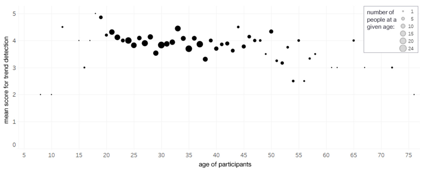
To check for effects related to age, we derived five evenly spaced age groups accommodating the range between the youngest (8 years) and the oldest (76 years) participant. Using the npmv package for R again, those groups were tested on differences in scoring. When using all five age groups, there are highly significant differences for trend scores (p = 0.006), decreasing with age (Figure 10). As the highest (62.4–76) age group is rather small (7 participants), we dropped it due to potential statistical problems associated with highly different group sizes. Differences of the remaining four age groups are still highly significant (p =0.008). Trend scores are negatively correlated to age with a spearman’s rho (rs) of −0.14.
There is also a similar tendency according to outlier scores, although not significant. We further did not find significant differences of outlier- and trend scores for sex, map use experience, educational level, computer gaming frequency, nor for paid (crowdworkers) versus voluntary participation.
3.4. Self-Confidence
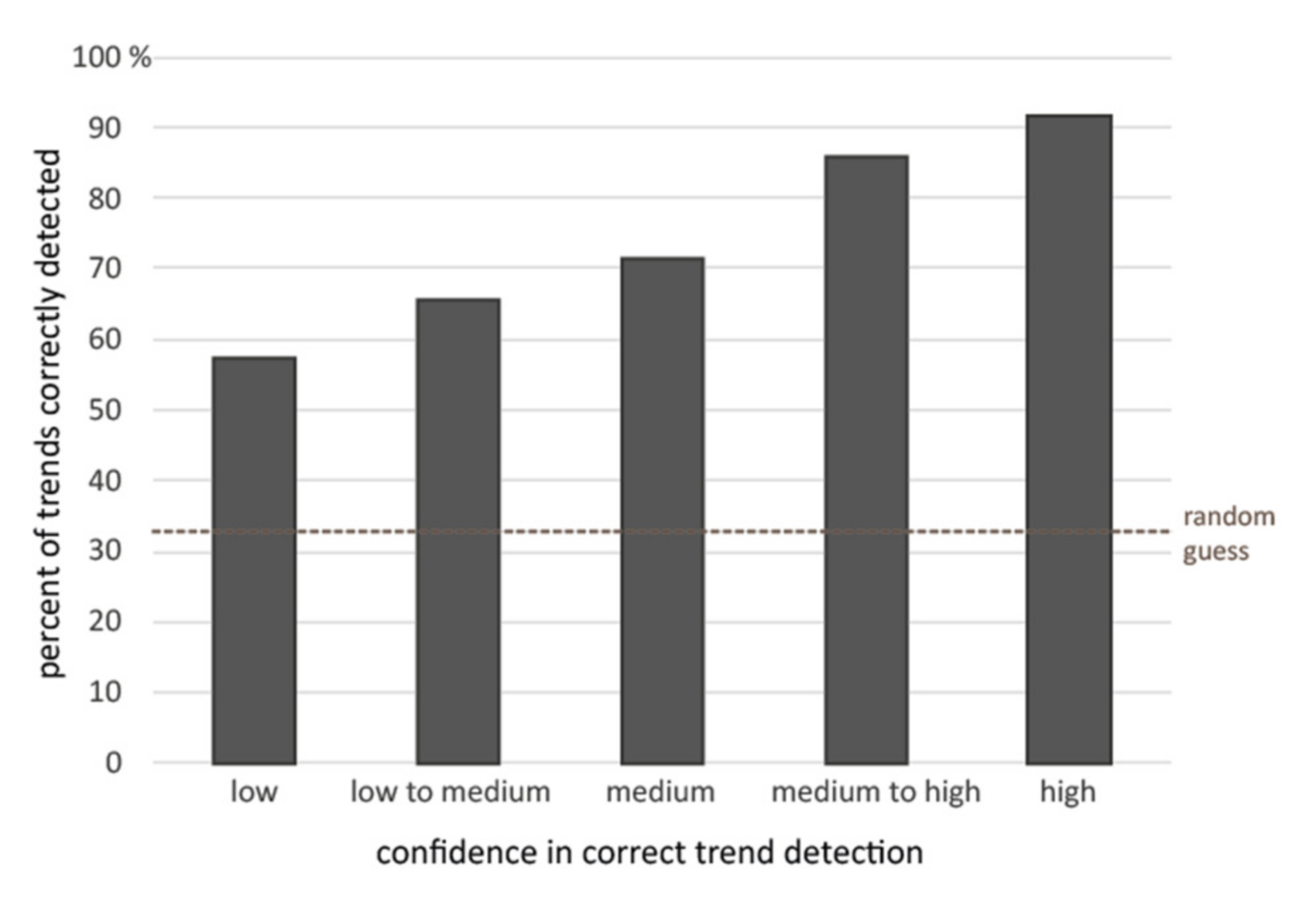
Self-confidence ratings are positively correlated to the actual capability to correctly detect trends (rs = 0.30) and outliers (rs = 0.55). Under the condition of low confidence in the personal choice, a hit rate of 58% in trend-detection seems to be quite high (Figure 11). On the other hand, 8% of the according decisions were still wrong, although participants were highly confident to be right. In the case of outlier detection, the rate of misses (for having both outliers correct) increases up to 19% under the highest confidence rating (Figure 12). Thus, people do seemingly overestimate their visual detection abilities as described by Levin et al. [31].
3.5. Strategies for Perception and Memorization
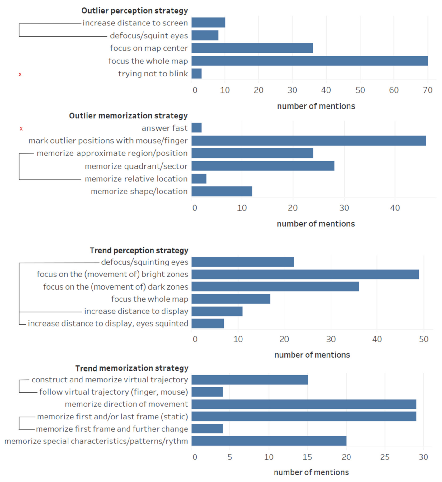
Qualitative answers on strategies for outlier and trend detection were split into perception and memorization strategies and clustered into categories (Figure 13).
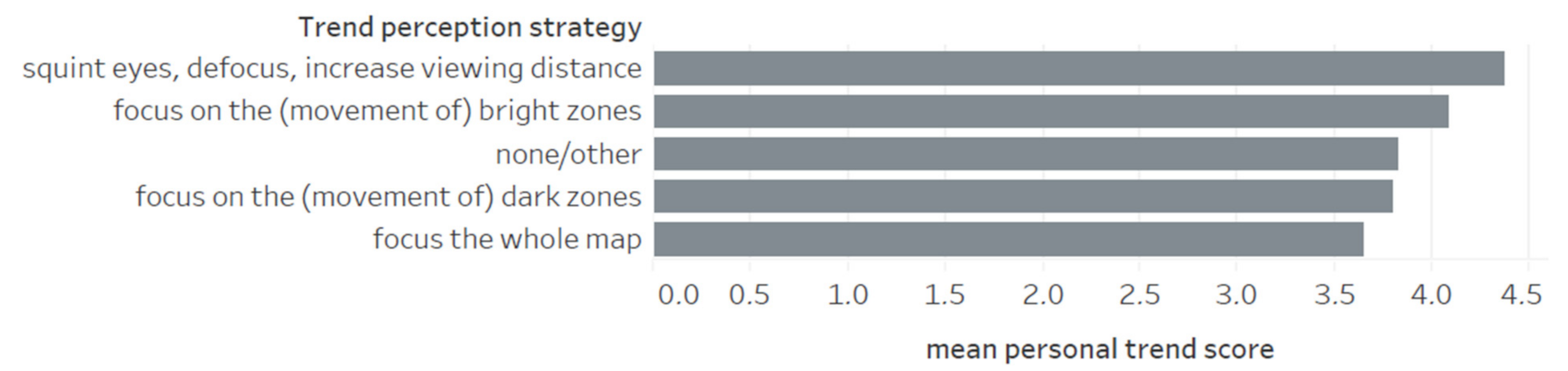
As we wanted to test the effectiveness of the strategies mentioned and thus strived for group sizes with higher statistical reliability, we further aggregated related categories like “construct and memorize virtual trajectory” and “follow virtual trajectory (finger, mouse)” or excluded them (“try not to blink”, “answer fast”) from analysis as indicated in Figure 13. Outlier detection and memorization strategies were tested for differences in personal outlier scores and trend related strategies for differences in personal trend scores, respectively. While we did not find significant impacts of outlier perception/memorization and trend memorization strategies on user performance, trend perception strategies resulted in significantly different scores (p = 0.016). Among those strategies, squinting the eyes, defocusing the map, and/or leaning back while watching the animation worked best (Figure 14).
3.6. Described Perception and Preference
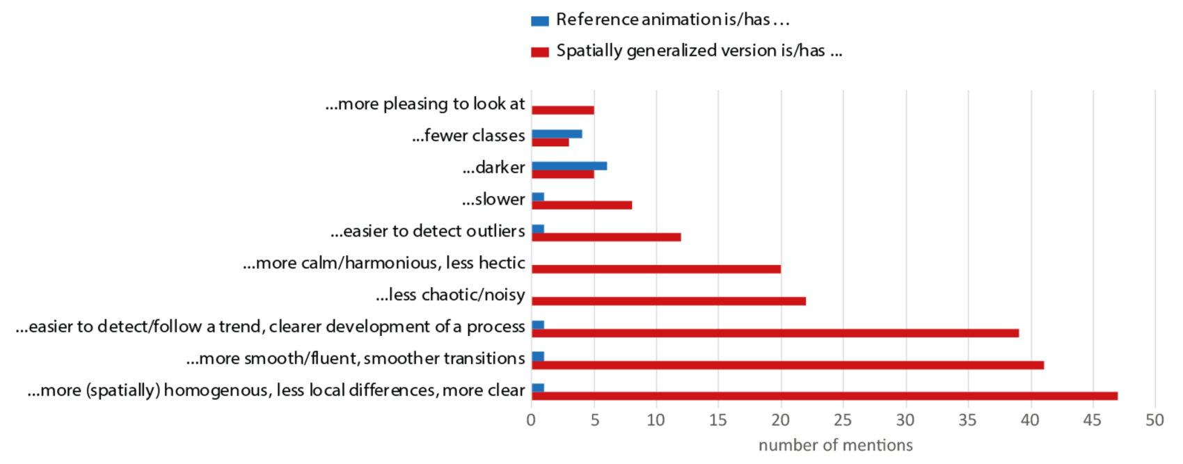
In our pilot study, participants were asked to verbally describe the difference between a reference animation (“Version A”) and its spatially generalized counterpart (“Version B”) using Stimulus 4. While 30% indicated to see no or only little differences, and 14% did not answer this open question, a content analysis of the remaining descriptions shows that the spatially generalized version was described to be more homogenous, smoother, less hectic, and less noisy. Furthermore, several persons emphasized that the generalized version facilitates the detection of a clear trend and/or local outliers thereof (Figure 15).
We noticed considerable differences in the individual ability to consciously see and describe differences between both versions: Some participants proposed the surprisingly correct assumption that version B might be a spatially generalized version from raw data shown in version A, and one of them even mentioned that outliers seem to be excluded from spatial smoothing. In turn, others reported to have repeatedly watched the animation loop for minutes without seeing any difference. After survey completion, a member of the latter group approached us, asking whether there was any difference. After explaining and showing the animation loop again, he was astonished to have missed the yet clearly seen differences beforehand. Arguing that he has been looking for changes on the level of individual polygons instead of the overall picture, different foci of visual attention, and thus inattentional blindness [32], might be the reason for the 30% share of participants who did not see any difference.
Regarding the question “Which version is easier to understand?”, participants from the pilot study clearly preferred the spatial generalized version (Figure 16). To foster involvement, we decided on an exclusive choice in this question, but provided the possibility to refuse but provide additional comments. Based on those comments, we created the categories “no preference” (people that saw the differences, but did not prefer either option), “no or minimal differences” (participants saw no or hardly any difference and thus cannot make a decision), and “no answer” (no comment). While typical comments of the group in favor of the spatially generalized version rephrase the verbal descriptions from above, the “no preference” group often answered in an “it depends” fashion, emphasizing different goals (general overview versus local detail) of an animation.
4. Discussion
Our experiments document that local outlier excluding generalization of highly autocorrelated animated choropleth maps is (a) effective for emphasizing local outliers, and (b) works best when performed in the spatial dimension. It also suggests that map users prefer noise reduced animations. Nevertheless, assumed improvements in trend detection are not confirmed by the data, although roughly 10 percent of the participants from the pilot study explicitly mention a perceived facilitation in this respect. While the results suggest that the personal ability to identify local outliers and global trends in the used map animations does not depend on sex, cartographic experience, gaming affinity, or educational level, it seems that age and trend detection strategies play a significant role for trend detection. In the following, those results are further discussed.
4.1. Local Outlier Detection
Searching for and attending to objects from a visual scene is thought to be an interplay of bottom-up and top-down processes of vision [33]. Which group of processes dominates largely depends on the actual task. Tasks heavily based on prior knowledge about the world, like searching the desk in need of a pen (instead of searching the picture above, even if it is much more salient than the desk), top-down-processes will dominate where we attend to and direct our gaze at.
Conversely, in uninformed discovery of completely new visual information, bottom-up processes driven by the heterogeneity of the visual field itself play the leading role. Areas that “pop-out” by being different in intensity, color, or orientation are more likely to “catch the eye” than areas with little local contrast. The local intensity of perceptual conspicuousness or, in other words, the “physical attraction” of each region within the field of view can be described by visual saliency models that are based on neuroanatomical and physiological knowledge about our visual system [34,35]. Implementations of such models [36,37,38] produce saliency maps of visual scenes, estimating the perceived visual salience of objects within photos, videos, or even maps in a geographic sense [39,40]. When using saliency maps to predict eye fixation points and thus overt visual attention of test persons, best predictions were achieved when subjects explicitly had to search for high salience in the scene, followed by free viewing tasks and a search for predefined but salient objects [41]. The task of uninformed looking for two local outliers as features of highest local contrast in color/lightness might lie somewhere between direct salience search and salient object search. Thus, we consider the visual saliency of local outliers being decisive for their detection in choropleth map animations.
Visual salience does not only increase with the individual difference of a target object (in our case a local outlier) to other objects (neighboring polygons), but also with the homogeneity of those potentially distracting objects [33,42]. Changes in distractor homogeneity without affecting distractor–target difference might happen in cases where a different visual variable separates the target from distractors. As (our) local outliers differ from non-outlier polygons only in the amount of local color/lightness contrast, both modes of outlier saliency increase (increased target-distractor difference, increased distractor homogeneity) will operate simultaneously, if local contrast between distractors is reduced.
On the physiological level of color perception, simultaneous contrast also needs to be considered. Simultaneous contrast is commonly referred to as a shift of the brightness and the hue of an object towards the complementary brightness and hue of the surrounding area [43], perceptually enhancing color contrast and thus facilitating object delineation. Often, this is illustrated by pointing to different percepts of the same physical color in differently colored, uniform surroundings. Using this simple model of simultaneous contrast, it points to a perceptual gain of overall color contrast in the non-generalized stimuli, except for already rather uniform regions. Perceptual amplification of local contrast is therefore reduced between spatially smoothed neighbors. The perceived color of a local outlier would, however, hardly be affected by slight color adaptions among surrounding neighbors as the mean hue and brightness stays relatively constant. Thanks to the advice of a reviewer, we came across the work of Brown and MacLeod [44], who show that color appearance is also a function of the variance of surrounding colors. Colors appear more vivid against a low contrast surrounding than against heterogeneous, high contrast surroundings, even if the space-averaged, surrounding means are identical. Thus, the salience of local outliers is further enhanced by spatial-generalization of neighbors, due to mechanisms of this special type of simultaneous contrast.
Studies in visual search show an inverse relation of target salience and search time needed [45]. Thus, the probability to detect a local outlier in a given time (namely the duration of its existence within the animation) will increase with its salience. This explains the higher performance in outlier detection based on the spatially generalized choropleth map animations, which provide elevated outlier salience by reduced local contrast of distractor-polygons.
However, why does this mechanism not work similarly well when reducing local noise in time while preserving the large lightness changes of local outliers? Traun and Mayrhofer [26] calculated metrics on spatial and temporal map complexity for classed choropleth time series maps and their spatial, temporal, and spatiotemporally generalized variants, respectively. While visual complexity unsurprisingly decreased in the dimension (space/time) used for data smoothing, complexity increased in the unused dimension. Only for the spatiotemporally generalized variant, they reported a (comparably slight) decrease in both spatial and temporal complexity. Implicitly assuming that spatial and temporal complexity similarly affect perception, they favored the spatiotemporal variant. Contrary to this, our results suggest that spatial complexity reduction has a much higher impact on local outlier detection ability than a decrease of complexity in time. Temporal smoothing of individual polygons seemingly reduces the spatial coherence of animations, which explains the increase in spatial complexity measures reported by Traun and Mayrhofer [26]. Generalization in individual lightness transitions seems to be rather irrelevant, as we most probably do not “see” choropleth map animations as spatially unrelated sets of “locations” separately changing over time, but as an inherently spatial yet dynamically changing visual field, from which we perceptually delineate dynamic objects of higher order (regions) based on local contrast differences (especially contrast edges) in space. Such a view does not only conform to the theory of perceptual object formation as proposed by Gestalt psychology [46]. It also makes sense from an evolutional–functional perspective on vision in facilitating interaction with a world of three-dimensional objects. Although some of these objects might show an appearance or movement, their primary organizational structure is spatial, not temporal. Interestingly (or consequently?), the neural architecture of our visual system reflects the spatial layout of our visual field [47]. Along the stages of visual processing from retinal receptive fields through the lateral geniculate nucleus, the primary visual cortex and several subsequent cortical areas dedicated to vision, the spatial arrangement of neurons preserves the spatial arrangement of ganglion cells in the retina. Nearby locations in our visual field are thus processed by nearby neurons in a number of visual field maps within our brain [48].
In the main study, participants were informed that each stimulus contains exactly two outliers. Disclosing this information, we reacted to several comments from the pilot study where participants were left in uncertainty about this fact. While many of those complained about the overall difficulty of the task, others implicitly revealed that they assumed to find two outliers after having worked through the first stimuli. Therefore, we decided to remove this additional level of complexity in the main study. Despite this and other changes in the final study design, the results of the pilot study closely resemble the patterns observed in the main study for correct outliers and false-positives (best performance of the spatial generalization variant, no significant difference between reference and temporal variant and the spatiotemporal version somewhere in-between).
4.2. Global Trend Detection
Change in the global trend of spatiotemporally highly autocorrelated choropleth map animations is perceived as motion. The impression of a “moving front”, the “expansion of high value areas” or the “movement of a cluster of low values” is rooted in the conveyed connectivity by the contiguous borders [23] and the overall gradually changing lightness in space and time. As we assimilate regions of similar lightness to perceptual figures with borders defined by steeper color gradients, the underlying spatial process—like the outbreak of an infectious disease expressed by locally expanding incidence rates—leads to the impression of border movement (e.g., movement of the epidemic front), although only the lightness of individual polygons changes in a coordinated way. Depending on the perceived motion directions of all of its borders, the bounded figure virtually grows, shrinks, or moves. In comparison, the spatially separated symbols of an animated proportional symbol map do not provide such strong perception of “underlying motion” [23], nor would it result from choropleth map animations of data with little autocorrelation in space or time. In the latter case, the underlying process or the chosen scale of aggregation simply provides too little coherence within individual lightness changes, leading to increasing numbers of appearing and disappearing figures, quickly exceeding our cognitive capacities.
Another important factor for apparent motion is animation speed. In their comparative study on the detection of space-time clusters in small multiples and animated maps, Griffin, et al. [49] found that the apparent movement and thus the detection rate of clusters was closely related to animation pace. They plausibly hypothesize, that the gestalt grouping principle of common fate [46] cannot be established by our visual system if the animation runs too slow, while cognitive processing cannot keep up, if it is too fast. While we did not vary animation speed in our experiment, overall global trend detection rates were rather high (Figure 9). Thus, we assume that animation speed was within an appropriate range for detection of apparent motion.
In our experiment, generalization did not significantly improve the ability of participants to assign the correct blurred trend candidate to the respective stimulus, although 11% of participants emphasized a subjectively easier to follow trend in the spatially generalized animation in the pilot study.
A possible explanation for the negative quantitative results regarding our hypothesis that improved local homogeneity improves trend perception is the human ability to attend to distinct spatial frequencies and efficiently filter visual noise at spatial frequency levels that are not attended [50,51]. According to Snowden, Thompson, and Troscianko [47], keeping eyes squinted or increasing viewing distance facilitates the perception of low spatial frequencies. Therefore, it is not surprising that the intuitive adoption of exactly these strategies significantly facilitated trend perception. The superior performance of the group having focused on bright zones over the followers of the dark zones is in line with literature too. Nothdurft [52] found that bright targets are more salient among dark targets than vice versa.
It turned out that trend detection abilities in choropleth map animations are decreasing with age. Although the decline is moderate, it is highly significant. In view of general perceptual and cognitive changes across the human lifespan, this result is not surprising. From a psychophysiological perspective, general trend detection primarily seems related to the perception of motion coherence and translational motion (in opposite to the radial flow we experience when moving through the environment or biological motion, elicited by body movements of human figures). Both modes of motion perception decline with age [53,54], thus our findings are in line with the respective literature.
5. Conclusions and Outlook
We conclude that outlier preserving value generalization in space facilitates the identification of local outliers in choropleth map animations, while we could not find such an effect for generalization in time.
Our overall negative results on the benefit of temporal smoothing of choropleth map animations complement similar findings by McCabe [23] for different map use tasks. Like us, he used unclassed choropleth maps for his experiment. If the transfer of these findings to classed choropleth map animation holds, the according complexity metrics as introduced by Goldsberry and Battersby [2] needed to be rethought, as they solely depend on (class) changes of individual polygons in time. As a reduction in temporal complexity does not seem to improve perception, the question arises, whether purely temporal complexity metrics are a useful proxy for the perceived complexity of animated choropleth maps. Indices based on composite “perception objects” that have been segmented directly from spatiotemporal data or from the output of dynamic saliency models [55] might be a first step towards a more adequate description of animated map complexity. The development of according algorithms and tools to estimate the perceptibility of animated choropleth maps offers ample room for future research.
In their study mentioned above, Griffin, MacEachren, Hardisty, Steiner, and Li [49] noticed, that the optimal animation pace for apparent motion detection was different for various cluster intensities. This clearly prompts for interactive control of the animation speed by the user, but also shows how sensitive perceptual grouping by common fate is regarding animation speed. The complex relations between animation speed and different degrees of spatial and temporal autocorrelation on the perception of apparent motion in animated choropleth maps still waits to be fully uncovered. While we did not find evidence for benefits of value generalization for global trend detection, it cannot be excluded that this also holds true in situations where apparent motion is harder established due to noisier conditions, less “coordinated” color changes or due to suboptimal animation speed for detecting a certain spatial process.
Author Contributions
Conceptualization, investigation, writing of the original and revised draft, visualization, Christoph Traun; statistical data analysis, Manuela Larissa Schreyer and Christoph Traun; software for stimulus generation, Gudrun Wallentin. All authors have read and agreed to the published version of the manuscript.
Funding
Except for publication support by the Open Access Publication Fund of the University of Salzburg, this research received no external funding.
Institutional Review Board Statement
Not applicable.
Informed Consent Statement
Not applicable.
Data Availability Statement
Map stimuli, response items, and the analyzed, yet anonymized, dataset from the main study are available at https://tinyurl.com/mapstudyresults.
Acknowledgments
The main author likes to thank Wolfgang Trutschnig for his valuable discussion on the study design, the anonymous reviewers for their helpful inputs, and the voluntary participants for their kind engagement in the experiment. All authors acknowledge financial support by the Open Access Publication Fund of the University of Salzburg.
Conflicts of Interest
The authors declare no conflict of interest.
References
- Harrower, M. The Cognitive Limits of Animated Maps. Cartographica 2007, 42, 349–357. [Google Scholar] [CrossRef]
- Goldsberry, K.; Battersby, S. Issues of Change Detection in Animated Choropleth Maps. Cartogr. Int. J. Geogr. Inf. Geovis. 2009, 44, 201–215. [Google Scholar] [CrossRef] [Green Version]
- DuBois, M.; Battersby, S.E. A Raster-Based Neighborhood Model for Evaluating Complexity in Dynamic Maps. In Proceedings of the AutoCarto 2012, Columbus, OH, USA, 16–18 September 2012. [Google Scholar]
- Rosenholtz, R. Capabilities and limitations of peripheral vision. Annu. Rev. Vis. Sci. 2016, 2, 437–457. [Google Scholar] [CrossRef] [Green Version]
- Sweller, J. Cognitive load during problem solving: Effects on learning. Cogn. Sci. 1988, 12, 257–285. [Google Scholar] [CrossRef]
- Sweller, J.; van Merriënboer, J.J.; Paas, F. Cognitive architecture and instructional design: 20 years later. Educ. Psychol. Rev. 2019, 31, 1–32. [Google Scholar] [CrossRef] [Green Version]
- Luck, S.J.; Vogel, E.K. The capacity of visual working memory for features and conjunctions. Nature 1997, 390, 279–281. [Google Scholar] [CrossRef]
- Metaferia, M.T. Visual Enhancement of Animated Time Series to Reduce Change Blindness. Master’s Thesis, University of Twente, Enschede, The Netherlands, 2011. [Google Scholar]
- Harrower, M.; Fabrikant, S.I. The role of map animation for geographic visualization. In Geographic Visualization. Concepts, Tools and Applications; Dodge, M., Derby, M.M., Turner, M., Eds.; John Wiley & Sons: Chichester, UK, 2008; pp. 49–65. [Google Scholar]
- Harrower, M. Tips for designing effective animated maps. Cartogr. Perspect. 2003, 63–65. [Google Scholar] [CrossRef]
- Kraak, M.-J.; Edsall, R.; MacEachren, A.M. Cartographic animation and legends for temporal maps: Exploration and or interaction. In Proceedings of the 18th International Cartographic Conference, Stockholm, Sweden, 23–27 June 1997; pp. 253–261. [Google Scholar]
- Midtbø, T. Advanced legends for interactive dynamic maps. In Proceedings of the 23th International Cartographic Conference “Cartography for everyone and for you”, Moscow, Russia, 4–10 August 2007; pp. 4–10. [Google Scholar]
- Muehlenhaus, I. Web Cartography: Map Design for Interactive and Mobile Devices; CRC Press: Boca Raton, FL, USA, 2013. [Google Scholar]
- Opach, T.; Gołębiowska, I.; Fabrikant, S.I. How Do People View Multi-Component Animated Maps? Cartogr. J. 2014, 51, 330–342. [Google Scholar] [CrossRef]
- Fish, C.; Goldsberry, K.P.; Battersby, S. Change blindness in animated choropleth maps: An empirical study. Cartogr. Geogr. Inf. Sci. 2011, 38, 350–362. [Google Scholar] [CrossRef]
- Battersby, S.E.; Goldsberry, K.P. Considerations in Design of Transition Behaviors for Dynamic Thematic Maps. Cartogr. Perspect. 2010, 16–32. [Google Scholar] [CrossRef]
- Cybulski, P.; Medyńska-Gulij, B. Cartographic redundancy in reducing change blindness in detecting extreme values in spatio-temporal maps. ISPRS Int. J. Geo-Inf. 2018, 7, 8. [Google Scholar] [CrossRef] [Green Version]
- Multimäki, S.; Ahonen-Rainio, P. Temporally Transformed Map Animation for Visual Data Analysis. In Proceedings of the GEO Processing 2015: The 7th International Conference on Advanced Geographic Information Systems, Applications, and Services, Lisbon Portugal, 22–27 February 2015; pp. 25–31. [Google Scholar]
- Monmonier, M. Minimum-change categories for dynamic temporal choropleth maps. J. Pa. Acad. Sci. 1994, 68, 42–47. [Google Scholar]
- Monmonier, M. Temporal generalization for dynamic maps. Cartogr. Geogr. Inf. Syst. 1996, 23, 96–98. [Google Scholar] [CrossRef]
- Harrower, M. Visualizing change: Using cartographic animation to explore remotely-sensed data. Cartogr. Perspect. 2001, 30–42. [Google Scholar] [CrossRef]
- Harrower, M. Unclassed animated choropleth maps. Cartogr. J. 2007, 44, 313–320. [Google Scholar] [CrossRef]
- McCabe, C.A. Effects of Data Complexity and Map Abstraction on the Perception of Patterns in Infectious Disease Animations. Master’s Thesis, The Pennsylvania State University, University Park, PA, USA, 2009. [Google Scholar]
- Ogao, P.J.; Kraak, M.J. Defining visualization operations for temporal cartographic animation design. Int. J. Appl. Earth Obs. Geoinf. 2002, 4, 23–31. [Google Scholar] [CrossRef]
- Slocum, T.A.; Slutter, R.S., Jr.; Kessler, F.C.; Yoder, S.C. A Qualitative Evaluation of MapTime, A Program For Exploring Spatiotemporal Point Data. Cartographica 2004, 39, 43–68. [Google Scholar] [CrossRef] [Green Version]
- Traun, C.; Mayrhofer, C. Complexity reduction in choropleth map animations by autocorrelation weighted generalization of time-series data. Cartogr. Geogr. Inf. Sci. 2018, 45, 221–237. [Google Scholar] [CrossRef]
- Moran, P.A.P. Note on Continuous Stochastic Phenomena. Biometrika 1950, 37, 17–23. [Google Scholar] [CrossRef]
- Crump, M.J.C.; McDonnell, J.V.; Gureckis, T.M. Evaluating Amazon’s Mechanical Turk as a Tool for Experimental Behavioral Research. PLoS ONE 2013, 8, e57410. [Google Scholar] [CrossRef] [Green Version]
- Team, R.C. R: A Language and Environment for Statistical Computing; R Foundation for Statistical Computing: Vienna, Austria, 2021. [Google Scholar]
- Ellis, A.R.; Burchett, W.W.; Harrar, S.W.; Bathke, A.C. Nonparametric inference for multivariate data: The R package npmv. J. Stat. Softw. 2017, 76, 1–18. [Google Scholar]
- Levin, D.T.; Momen, N.; Drivdahl, S.B.; Simons, D.J. Change Blindness Blindness: The Metacognitive Error of Overestimating Change-detection Ability. Vis. Cogn. 2000, 7, 397–412. [Google Scholar] [CrossRef]
- Simons, D.J. Attentional capture and inattentional blindness. Trends Cogn. Sci. 2000, 4, 147–155. [Google Scholar] [CrossRef]
- Wolfe, J.M.; Horowitz, T.S. Five factors that guide attention in visual search. Nat. Hum. Behav. 2017, 1, 0058. [Google Scholar] [CrossRef]
- Koch, C.; Ullman, S. Shifts in selective visual attention: Towards the underlying neural circuitry. Hum. Neurobiol. 1985, 4, 219–227. [Google Scholar] [PubMed]
- Veale, R.; Hafed, Z.M.; Yoshida, M. How is visual salience computed in the brain? Insights from behaviour, neurobiology and modelling. Philos. Trans. R. Soc. B Biol. Sci. 2017, 372, 20160113. [Google Scholar] [CrossRef]
- Bruce, N.D.; Tsotsos, J.K. Saliency, attention, and visual search: An information theoretic approach. J. Vis. 2009, 9, 5. [Google Scholar] [CrossRef]
- Itti, L.; Koch, C.; Niebur, E. A model of saliency-based visual attention for rapid scene analysis. IEEE Trans. Pattern Anal. Mach. Intell. 1998, 20, 1254–1259. [Google Scholar] [CrossRef] [Green Version]
- Zhang, L.; Tong, M.H.; Marks, T.K.; Shan, H.; Cottrell, G.W. SUN: A Bayesian framework for saliency using natural statistics. J. Vis. 2008, 8, 32. [Google Scholar] [CrossRef] [Green Version]
- Davies, C.; Fabrikant, S.I.; Hegarty, M. Toward Empirically Verified Cartographic Displays. In The Cambridge Handbook of Applied Perception Research; Szalma, J.L., Scerbo, M.W., Hancock, P.A., Parasuraman, R., Hoffman, R.R., Eds.; Cambridge University Press: Cambridge, UK, 2015; pp. 711–730. [Google Scholar]
- Fabrikant, S.I.; Goldsberry, K. Thematic relevance and perceptual salience of dynamic geovisualization displays. In Proceedings of the 22th ICA/ACI International Cartographic Conference, A Coruña, Spain, 9–16 July 2005. [Google Scholar]
- Koehler, K.; Guo, F.; Zhang, S.; Eckstein, M.P. What do saliency models predict? J. Vis. 2014, 14, 14. [Google Scholar] [CrossRef]
- Yantis, S. How visual salience wins the battle for awareness. Nat. Neurosci. 2005, 8, 975–977. [Google Scholar] [CrossRef]
- Slocum, T.A.; McMaster, R.B.; Kessler, F.C.; Howard, H.H. Thematic Cartography and Geovisualization, 3rd ed.; Pearson Prentice Hall: Upper Saddle River, NJ, USA, 2009. [Google Scholar]
- Brown, R.O.; MacLeod, D.I. Color appearance depends on the variance of surround colors. Curr. Biol. 1997, 7, 844–849. [Google Scholar] [CrossRef] [Green Version]
- Liesefeld, H.R.; Moran, R.; Usher, M.; Müller, H.J.; Zehetleitner, M. Search efficiency as a function of target saliency: The transition from inefficient to efficient search and beyond. J. Exp. Psychol. Human Percept. Perform. 2016, 42, 821. [Google Scholar] [CrossRef] [Green Version]
- Wagemans, J.; Elder, J.H.; Kubovy, M.; Palmer, S.E.; Peterson, M.A.; Singh, M.; von der Heydt, R. A century of Gestalt psychology in visual perception: I. Perceptual grouping and figure–ground organization. Psychol. Bull. 2012, 138, 1172–1217. [Google Scholar] [CrossRef] [Green Version]
- Snowden, R.; Thompson, P.; Troscianko, T. Basic Vision: An Introduction to Visual Perception; Oxford University Press: Oxford, UK, 2012. [Google Scholar]
- Wandell, B.A.; Dumoulin, S.O.; Brewer, A.A. Visual field maps in human cortex. Neuron 2007, 56, 366–383. [Google Scholar] [CrossRef] [Green Version]
- Griffin, A.L.; MacEachren, A.M.; Hardisty, F.; Steiner, E.; Li, B. A comparison of animated maps with static small-multiple maps for visually identifying space-time clusters. Ann. Assoc. Am. Geogr. 2006, 96, 740–753. [Google Scholar] [CrossRef] [Green Version]
- Shulman, G.L.; Sullivan, M.A.; Gish, K.; Sakoda, W.J. The Role of Spatial-Frequency Channels in the Perception of Local and Global Structure. Perception 1986, 15, 259–273. [Google Scholar] [CrossRef]
- Sowden, P.T.; Schyns, P.G. Channel surfing in the visual brain. Trends Cogn. Sci. 2006, 10, 538–545. [Google Scholar] [CrossRef] [Green Version]
- Nothdurft, H.-C. Attention shifts to salient targets. Vis. Res. 2002, 42, 1287–1306. [Google Scholar] [CrossRef] [Green Version]
- Billino, J.; Bremmer, F.; Gegenfurtner, K.R. Differential aging of motion processing mechanisms: Evidence against general perceptual decline. Vis. Res. 2008, 48, 1254–1261. [Google Scholar] [CrossRef] [Green Version]
- Snowden, R.J.; Kavanagh, E. Motion Perception in the Ageing Visual System: Minimum Motion, Motion Coherence, and Speed Discrimination Thresholds. Perception 2006, 35, 9–24. [Google Scholar] [CrossRef]
- Bak, C.; Kocak, A.; Erdem, E.; Erdem, A. Spatio-Temporal Saliency Networks for Dynamic Saliency Prediction. IEEE Trans. Multimedia 2018, 20, 1688–1698. [Google Scholar] [CrossRef] [Green Version]
Figure 1.
Slightly reduced local contrast in the spatially generalized version (right) of a frame from stimulus 1. The color of a local outlier polygon (bright polygon in the upper center) is not altered by generalization (left).
Figure 1.
Slightly reduced local contrast in the spatially generalized version (right) of a frame from stimulus 1. The color of a local outlier polygon (bright polygon in the upper center) is not altered by generalization (left).

Figure 2.
Local outlier response items for stimulus 1. Participants could choose between six outlier candidates (A–F). Option F shows the local outlier from Figure 1.
Figure 2.
Local outlier response items for stimulus 1. Participants could choose between six outlier candidates (A–F). Option F shows the local outlier from Figure 1.

Figure 3.
Global trend response item animations. As the six local outlier response items in the first part of the experiment, three trend response items immediately replace the seen stimulus in the second part of the study.
Figure 3.
Global trend response item animations. As the six local outlier response items in the first part of the experiment, three trend response items immediately replace the seen stimulus in the second part of the study.

Figure 4.
Study design.

Figure 5.
Age distribution by sex and group.

Figure 6.
Saturated bars show the number of crowdworker responses (33.4% of total) by sex and group. Compare to the proportion of other participants, depicted by the light bars.
Figure 6.
Saturated bars show the number of crowdworker responses (33.4% of total) by sex and group. Compare to the proportion of other participants, depicted by the light bars.

Figure 7.
Number of persons per group/generalization type for correctly detecting none, one, or both local outliers in each stimulus.
Figure 7.
Number of persons per group/generalization type for correctly detecting none, one, or both local outliers in each stimulus.

Figure 8.
Number of persons per group/generalization type for erroneously picking none, one, or two wrong outlier candidates (“false positives”).
Figure 8.
Number of persons per group/generalization type for erroneously picking none, one, or two wrong outlier candidates (“false positives”).

Figure 9.
Number of persons per group/generalization type having chosen the correct trend response item.
Figure 9.
Number of persons per group/generalization type having chosen the correct trend response item.

Figure 10.
Trend scores decrease with age. Personal trend scores are based on all stimuli and bounded by 0 (all trends incorrect) and +5 (all trends correctly detected). Participants of the same age are represented by one dot.
Figure 10.
Trend scores decrease with age. Personal trend scores are based on all stimuli and bounded by 0 (all trends incorrect) and +5 (all trends correctly detected). Participants of the same age are represented by one dot.

Figure 11.
Hit rates for different levels of confidence in correct trend detection.

Figure 12.
Hit rates and false alarms for different levels of confidence in correct outlier detection.
Figure 12.
Hit rates and false alarms for different levels of confidence in correct outlier detection.

Figure 13.
Strategies for outlier and trend detection and memorization.

Figure 14.
Performance of strategies for trend perception.

Figure 15.
Number of comparative mentions in verbal descriptions of differences between the reference animation and its spatially generalized counterpart of Stimulus 4. Classification was done semantically, e.g., “Version A is more chaotic than version B” is classified as “Spatially generalized version (B) is less chaotic”. In addition to these 217 comparative statements, 25 statements like “In version B the bright yellow seems to move farther up north” could not be attributed in a comparative way and were omitted.

Figure 16.
Answers for “Which version is easier to understand?” Absolute counts, n = 334.


Table 1.
Cartographic competence—absolute counts.
| Group A | Group B | Group C | Group D | ∑ | |
|---|---|---|---|---|---|
| None or little experience with maps | 17 | 12 | 17 | 11 | 57 |
| Active map use, no background in cartography | 35 | 38 | 34 | 44 | 151 |
| Basic knowledge in cartography | 37 | 34 | 30 | 23 | 124 |
| Advanced cart. knowledge, active mapping | 17 | 23 | 23 | 26 | 89 |
| Expert knowledge in cartography | 4 | 3 | 6 | 6 | 19 |
| ∑ | 110 | 110 | 110 | 110 | 440 |
Publisher’s Note: MDPI stays neutral with regard to jurisdictional claims in published maps and institutional affiliations. |
© 2021 by the authors. Licensee MDPI, Basel, Switzerland. This article is an open access article distributed under the terms and conditions of the Creative Commons Attribution (CC BY) license (http://creativecommons.org/licenses/by/4.0/).
Share and Cite
MDPI and ACS Style
Traun, C.; Schreyer, M.L.; Wallentin, G. Empirical Insights from a Study on Outlier Preserving Value Generalization in Animated Choropleth Maps. ISPRS Int. J. Geo-Inf. 2021, 10, 208. https://doi.org/10.3390/ijgi10040208
AMA Style
Traun C, Schreyer ML, Wallentin G. Empirical Insights from a Study on Outlier Preserving Value Generalization in Animated Choropleth Maps. ISPRS International Journal of Geo-Information. 2021; 10(4):208. https://doi.org/10.3390/ijgi10040208
Chicago/Turabian StyleTraun, Christoph, Manuela Larissa Schreyer, and Gudrun Wallentin. 2021. "Empirical Insights from a Study on Outlier Preserving Value Generalization in Animated Choropleth Maps" ISPRS International Journal of Geo-Information 10, no. 4: 208. https://doi.org/10.3390/ijgi10040208
Note that from the first issue of 2016, this journal uses article numbers instead of page numbers. See further details here.