
Assessment of Rainfall-Induced Landslide Distribution Based on Land Disturbance in Southern Taiwan

 ,
, 
Abstract
:1. Introduction
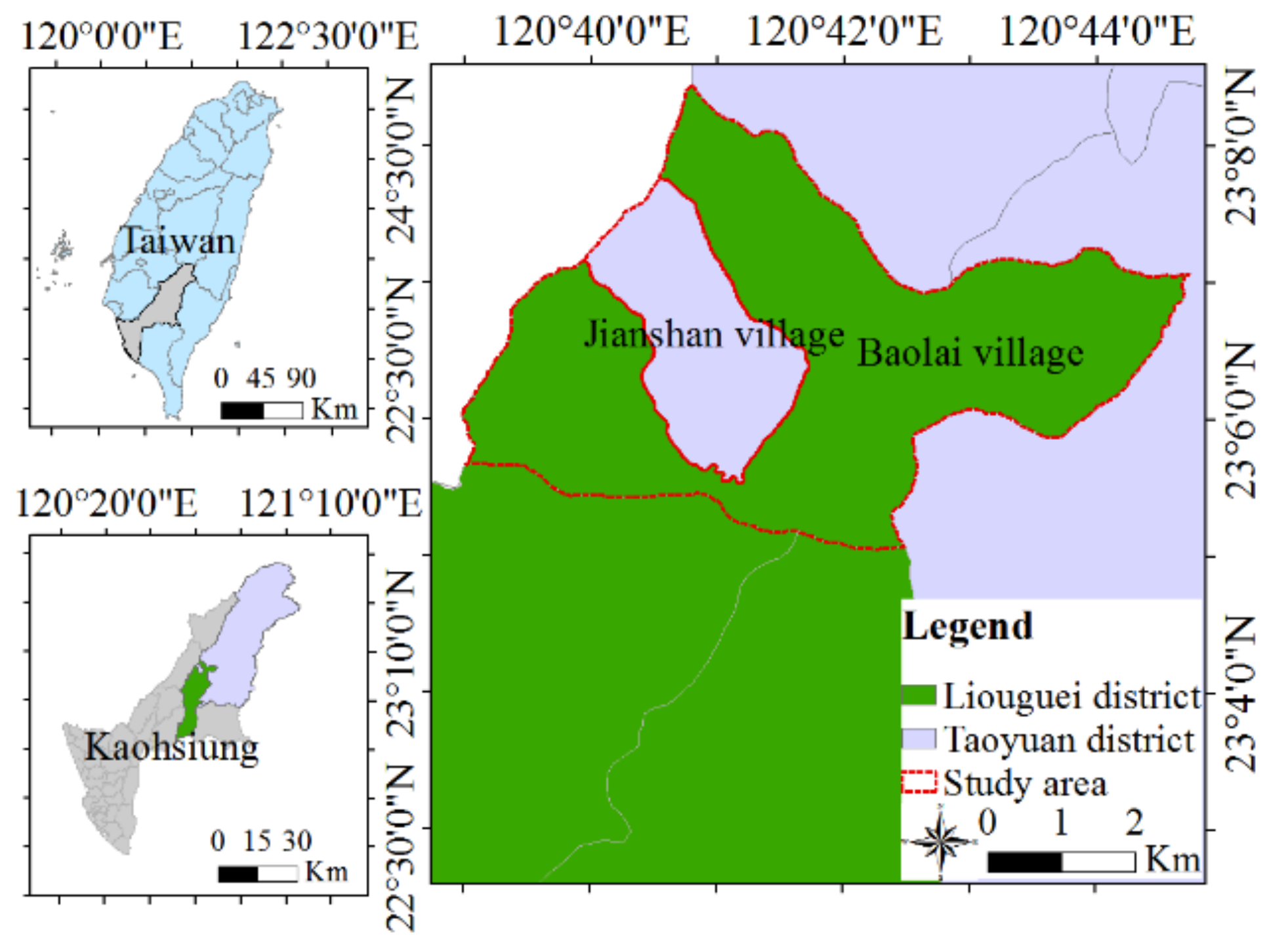
2. Study Areas
3. Methodology
3.1. Genetic Adaptive Neural Network
3.2. Texture Analysis
3.3. Accuracy Assessment
3.4. Accumulative Rainfall Analysis
3.5. GIS
4. Results
4.1. Construction of Original Cartographic Information
4.2. Establishment of Basic Grid
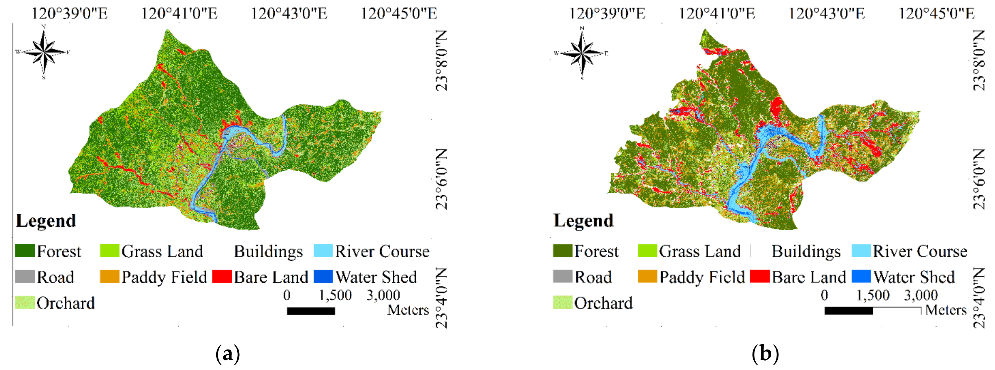
4.3. Interpretation and Classification of Satellite Images
4.3.1. Satellite Image Preprocessing
4.3.2. Satellite Image Interpretation and Classification
5. Discussion
5.1. Relationship between the Change in Bare Land and Topographic Location
5.2. Relationship between Bare Area, Quantity, and Rainfall
5.3. Relationship between the Number and Area of Bare Lands after Each Rainfall and the Degree of Slope Disturbance
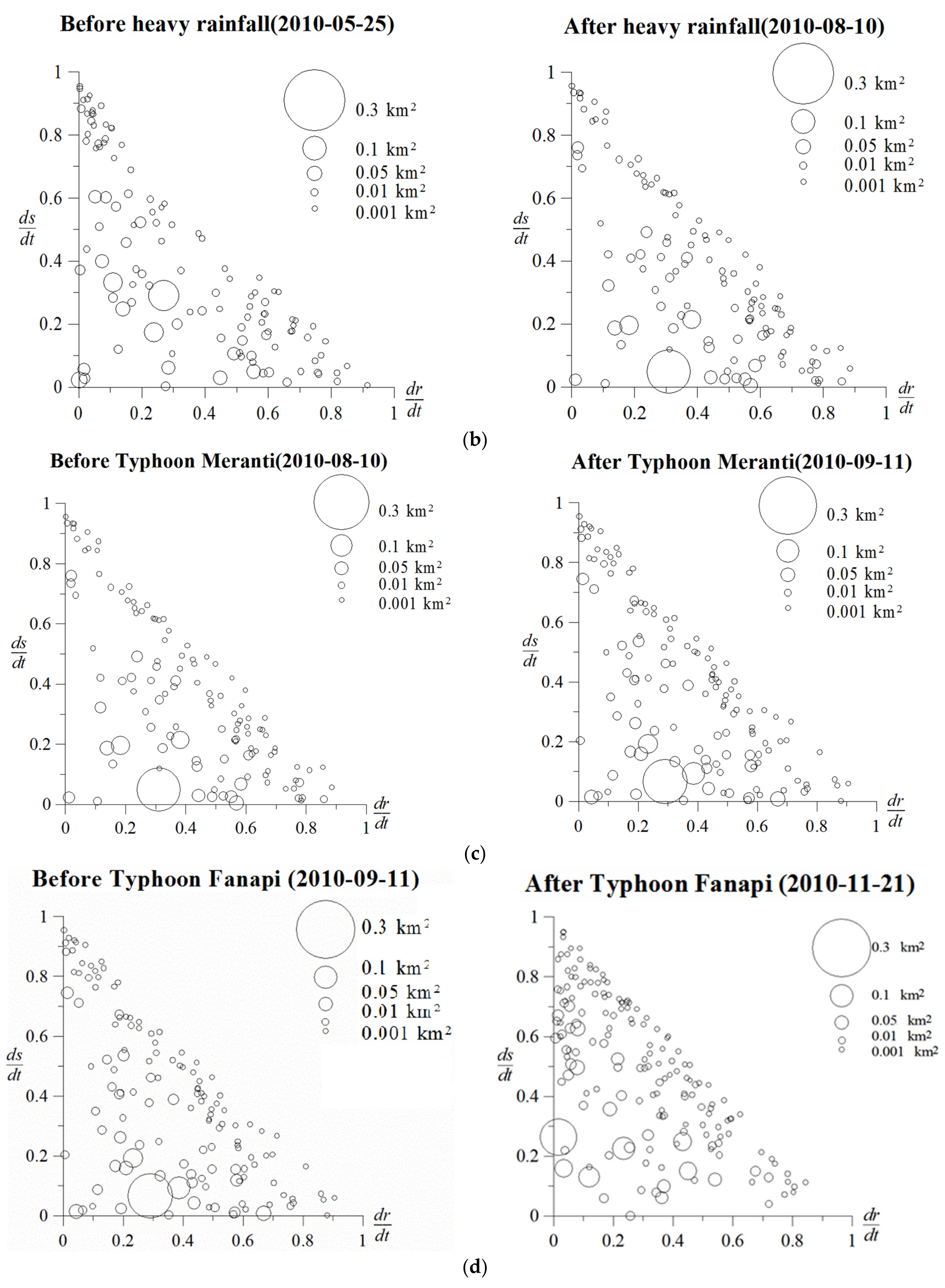
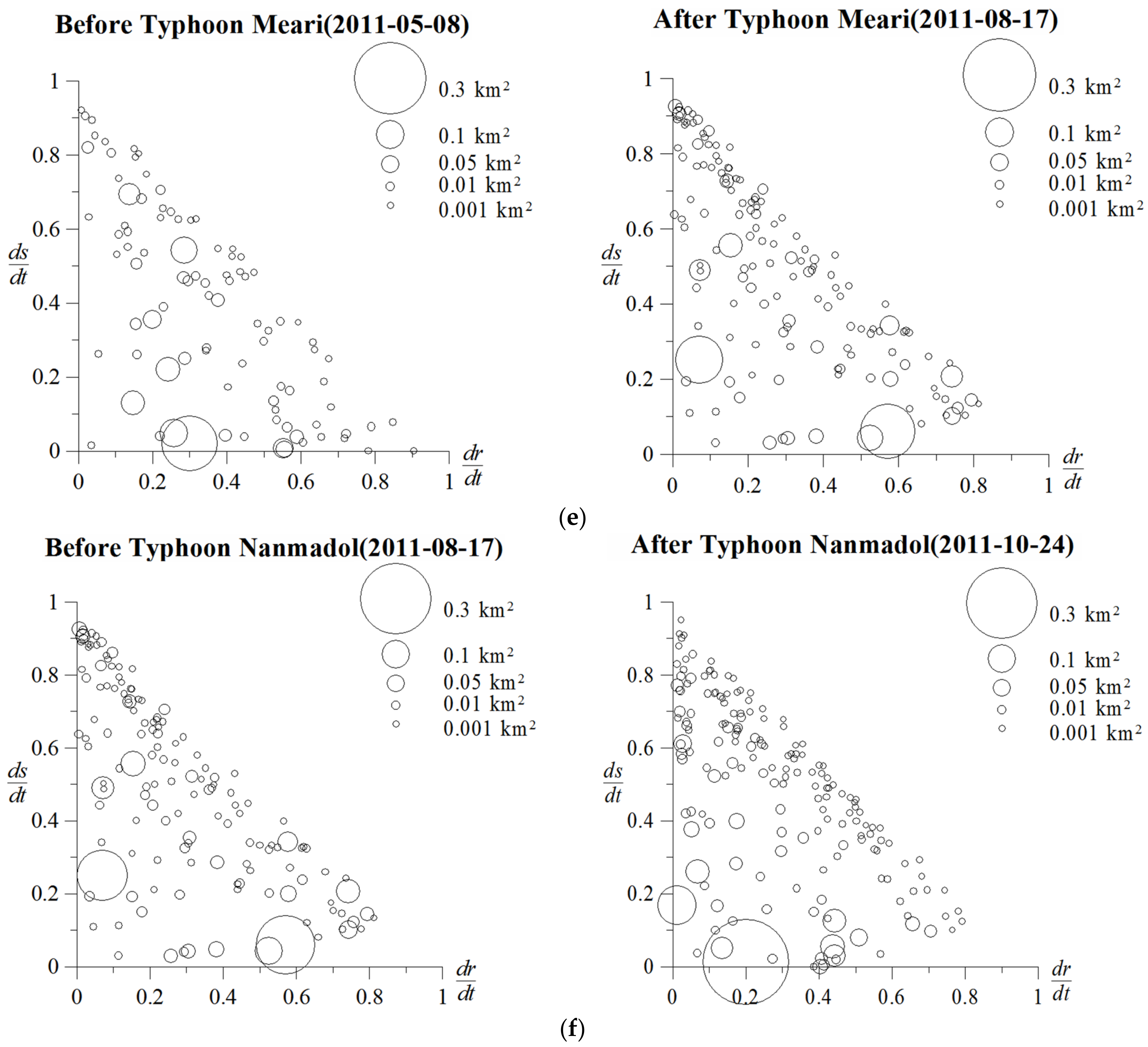
5.4. Relationship between the Scale of New or Second Landslide, Rainfall, and ILDC
5.4.1. Relationship between the Landslide Location and the Corresponding Landslide Area
5.4.2. Relationship between Landslide Area and Location, Rainfall, and Slope Disturbance
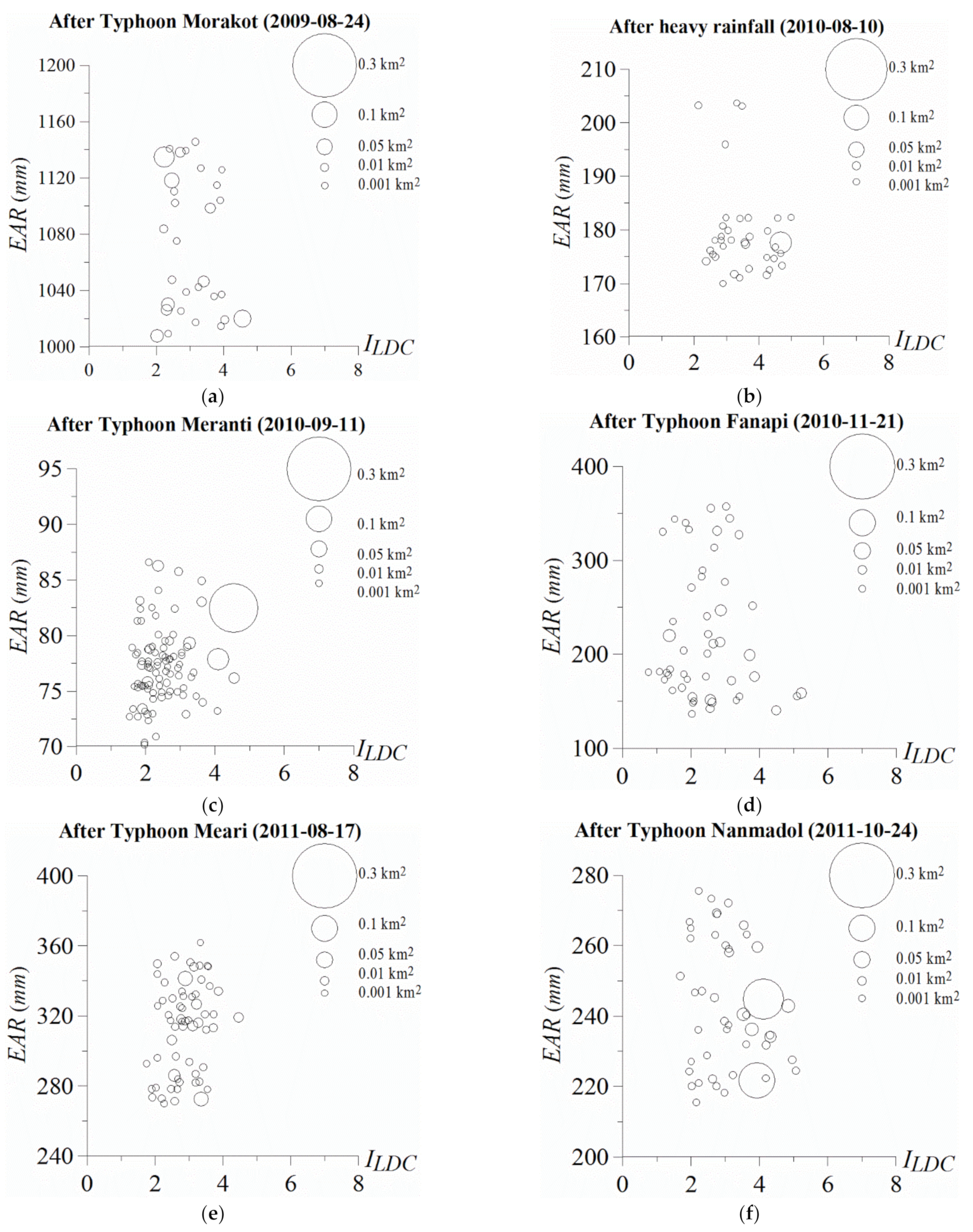
5.4.3. Relationship between Variation in Second Landslide Scale, Rainfall, and Slope Disturbance
6. Conclusions
- (1)
- For the interpretation and classification of high-resolution satellite images, this study used the GANN combined with texture analysis. The OA and consistency coefficient values of the interpretation results revealed that the satellite image interpretation before and after each rainfall in the research area achieved medium to high accuracy;
- (2)
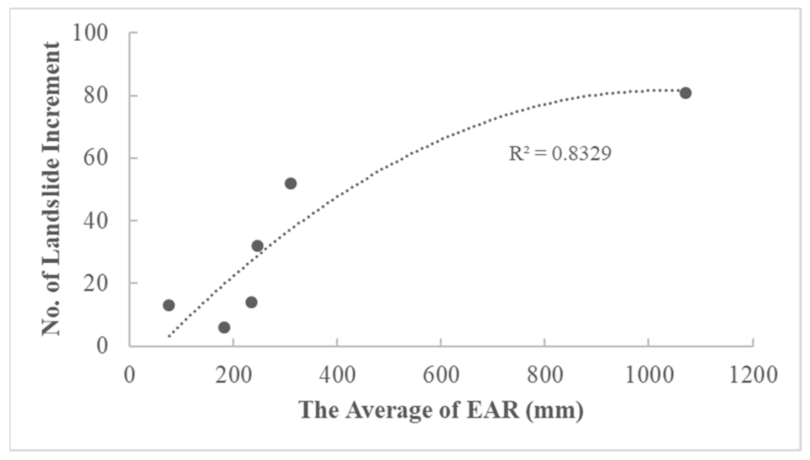
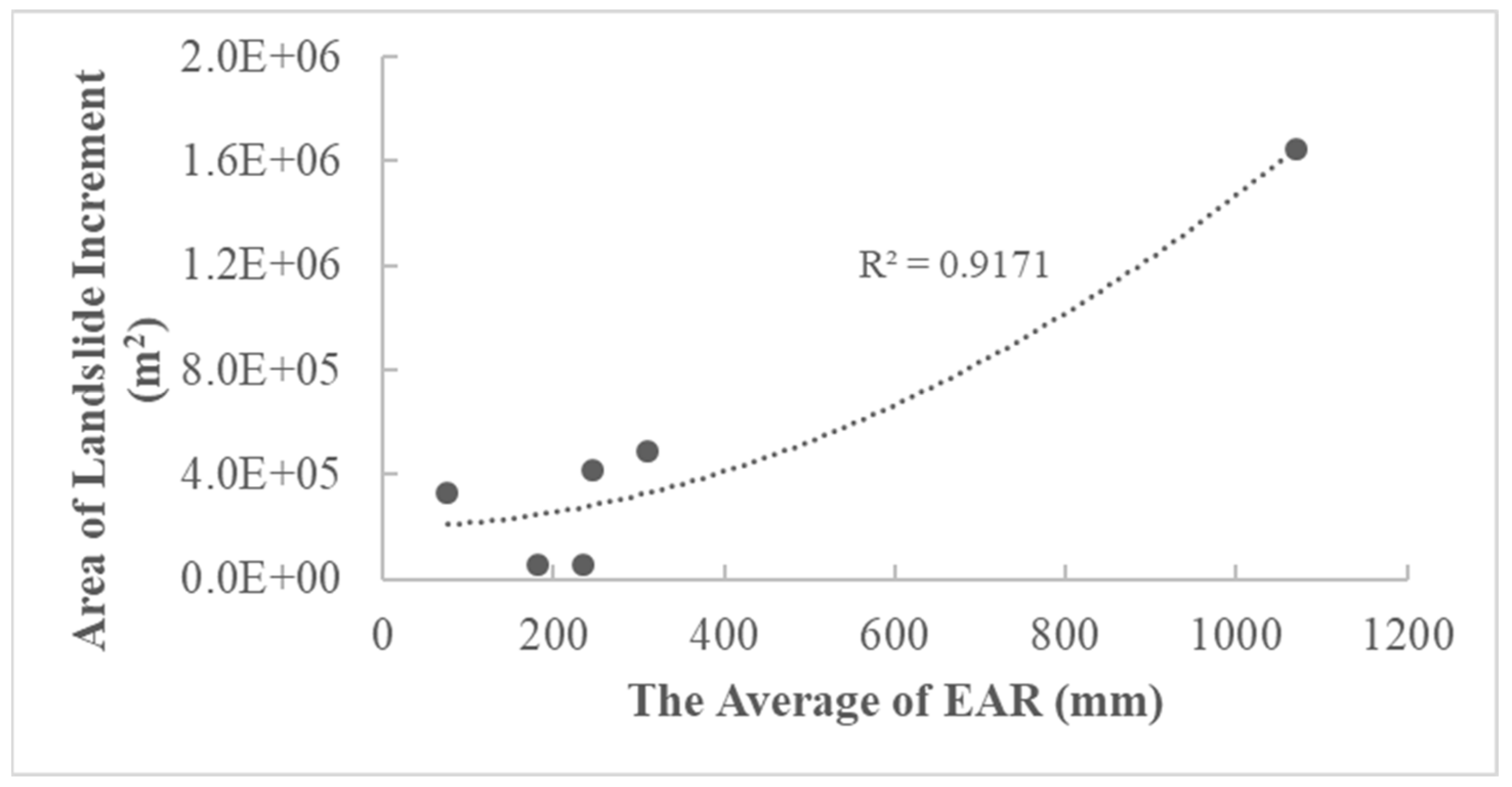
- A comparison of the number and area of the exposed areas before and after the six rainfalls revealed that the number or area of the bare land in the research area in each field significantly increased after the rainfall than before the rainfall. The distribution of bare land before and after Typhoon Morakot was the largest. In addition, after each rainfall, the number of bare lands and bare land areas increased with an increase in the average EAR. When the data were fitted with a polynomial trend line, the coefficient of determination between the average EAR and the increases in the number of bare lands and that between the average EAR and the increase in the landslide area was approximately 0.83 and 0.92, respectively;
- (3)
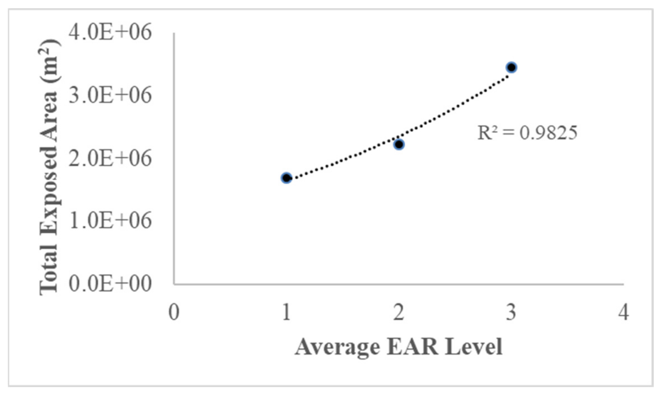
- In addition to the extreme rainfall during Typhoon Morakot in 2009, this study divided the average EAR after each rain into three levels in sequence and used the trend line of the exponential relationship to fit the bare land data. The results revealed that after each rainfall in the study area, the bare land area increased with an increase in the average EAR value, and the coefficient of determination of trend line reached 0.98;
- (4)
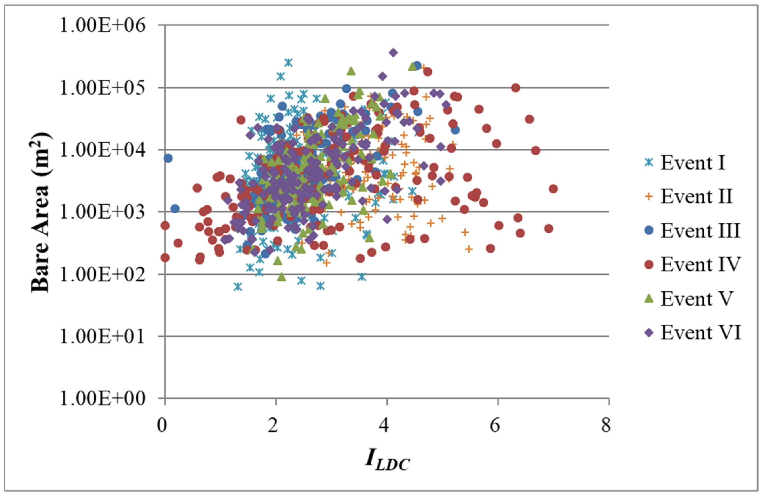
- The relationship between ILDC and the bare land area after each rainfall indicated that except for the extreme Morakot rains, the greater the degree of slope disturbance was after rain, the greater the area of the exposed slope was. This result also indicated that when extreme rainfall similar to Typhoon Morakot strikes, the impact of rainfall on the bare land area may be greater than the impact of slope disturbance. In addition, the results of the joint mapping study after the rainfall in each field revealed a positive relationship between the bare land area and ILDC;
- (5)
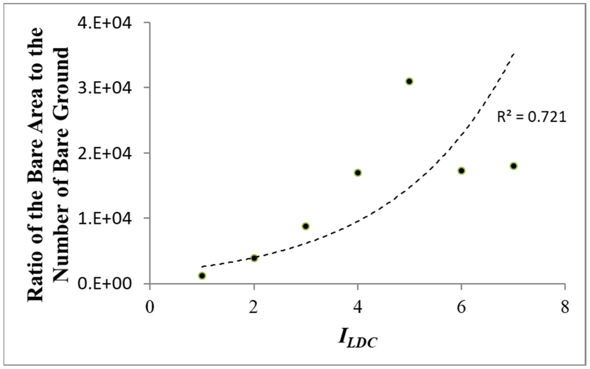
- The relationship between the ILDC in the study area and the ratio of the area of bare land to the amount of bare land after each rainfall indicated that the ratio of the area of bare land to the number of bare lands after each rainfall increased with ILDC;
- (6)
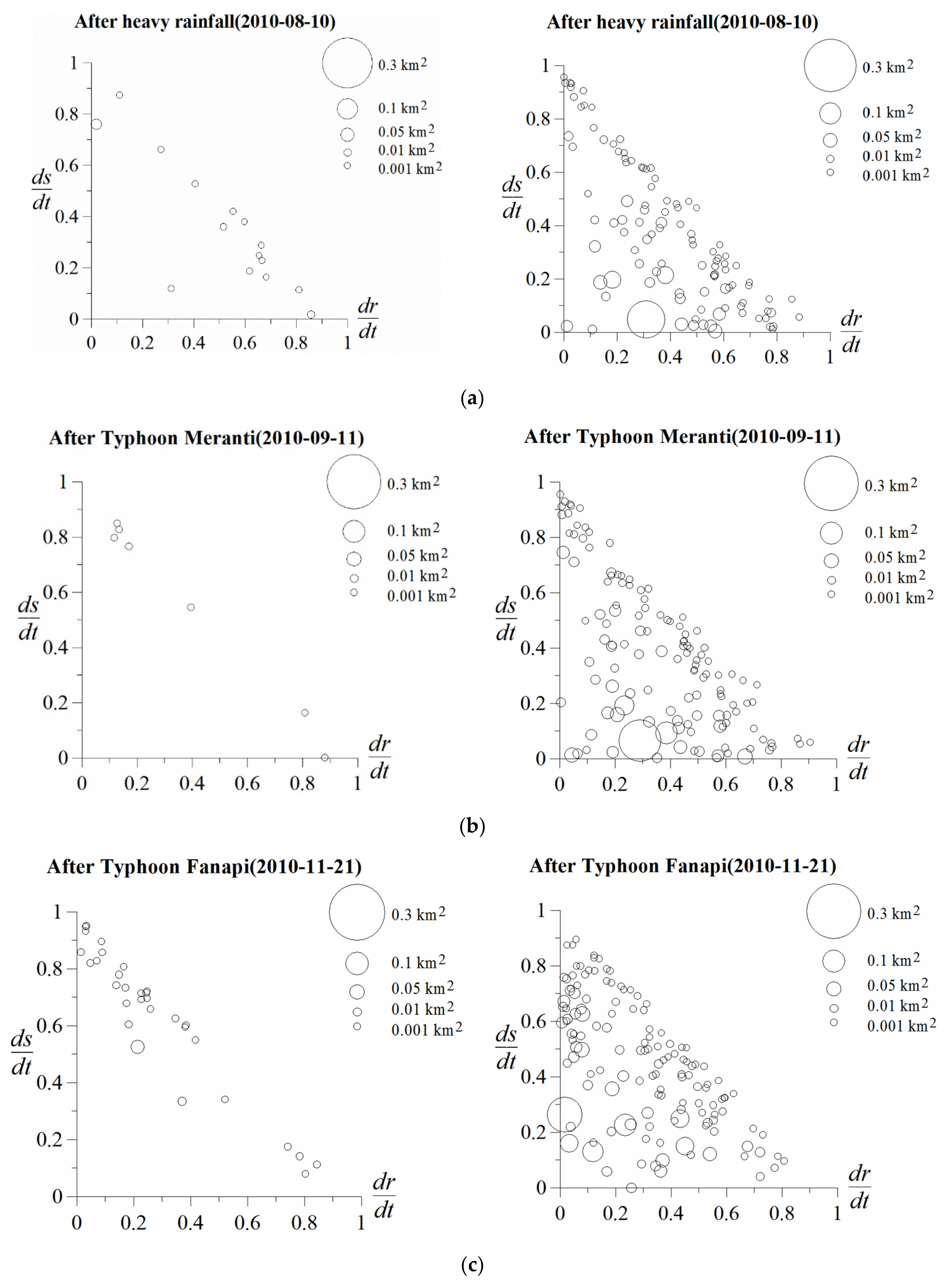
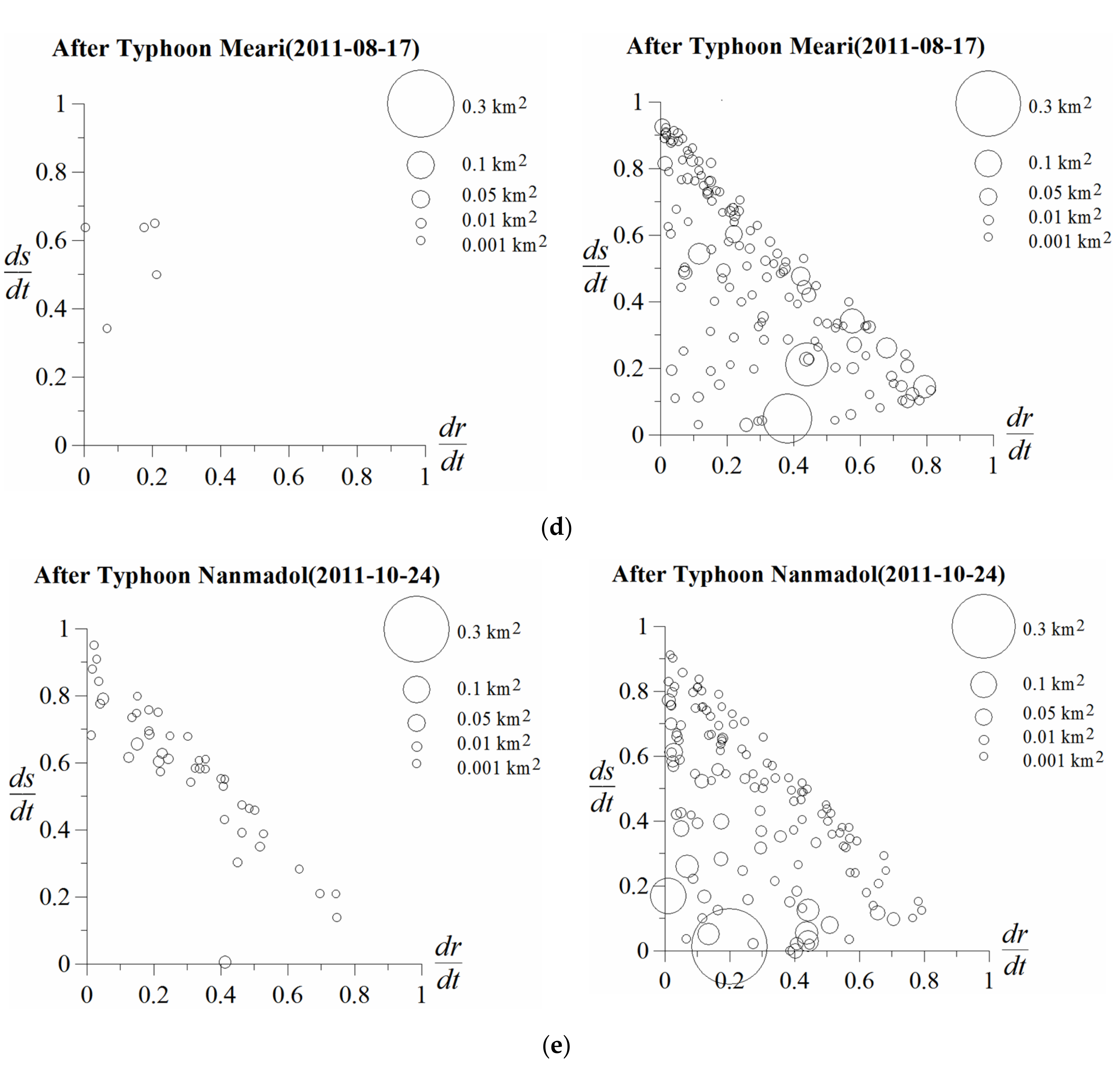
- The results of the rainfall-induced new landslide and second landslide in each field revealed that except for the number of new landslide points induced by the extreme rainfall event during Typhoon Morakot, which was considerably higher than the number of second landslide points, for the remaining landslides induced by rainfall, the number of second landslide points was higher than the number of new landslide points, and the area of the second landslide point was also greater than that of the new landslide point. In addition, despite the rainfall, the larger the slope disturbance, the larger the scale of the second landslide was. Consequently, more new landslide points were biased toward the ridge crest, whereas the second landslide points with larger landslide scales tended to develop toward the stream;
- (7)
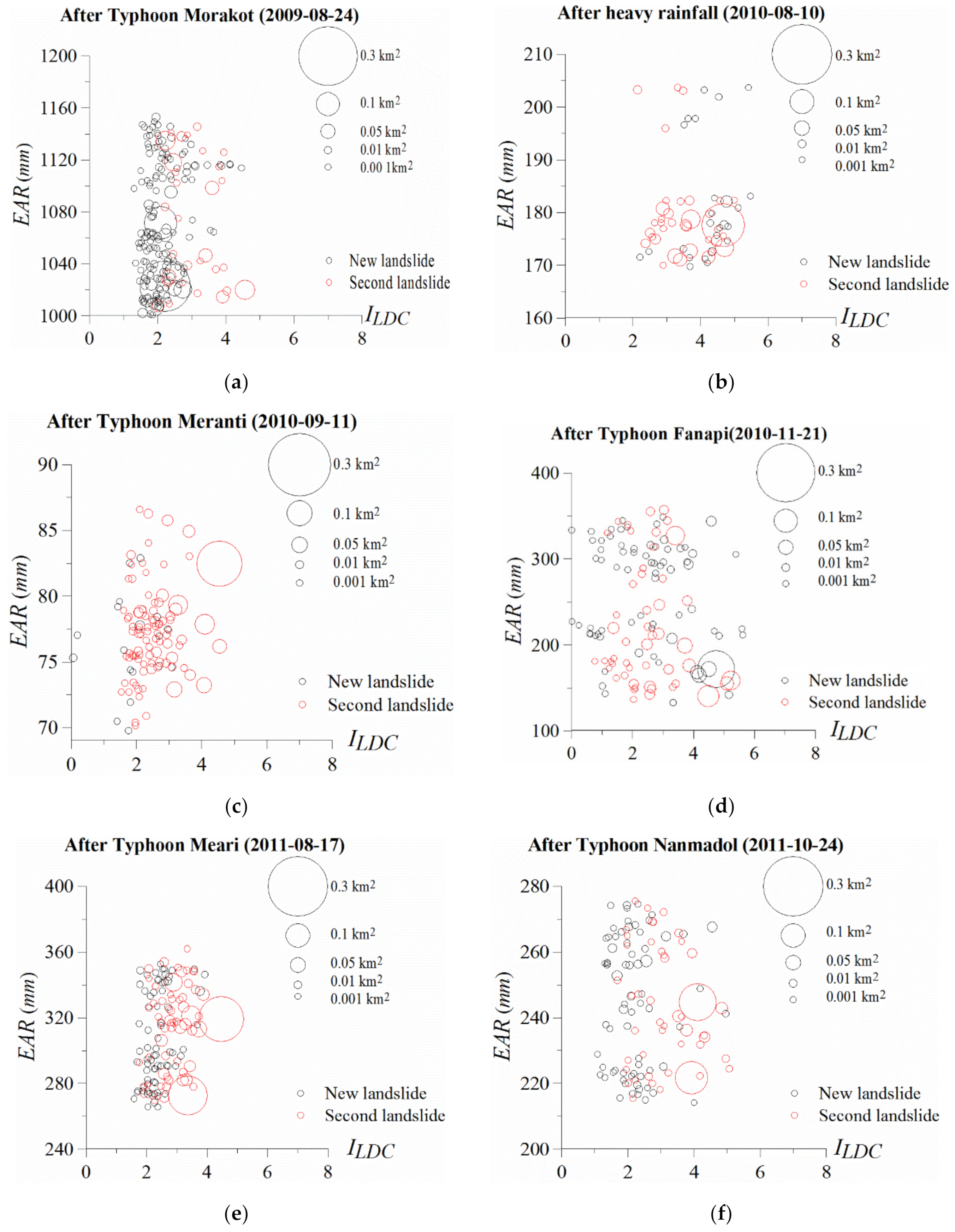
- After rainfall in each field, the relationship between the EAR at the point of the second landslide, ILDC, and re-increased area of landslide indicated that overall, a positive relationship was noted between the increased area of the landslide at the second landslide point and the EAR or ILDC. With an increase in the EAR on the slope in the study area or the slope disturbance, the area of the landslide at the second landslide point also tended to increase.
Author Contributions
Funding
Data Availability Statement
Acknowledgments
Conflicts of Interest
References
- Dadson, S.J.; Hovius, N.; Chen, H.; Dade, W.B.; Lin, J.C.; Hsu, M.L.; Lin, C.W.; Horng, M.J.; Chen, T.C.; Milliman, J.; et al. Earthquake triggered increase in sediment delivery from an active mountain belt. Geology 2004, 32, 733–736. [Google Scholar] [CrossRef]
- Lin, C.W.; Chang, W.S.; Liu, S.H.; Tsai, T.T.; Lee, S.P.; Tsang, Y.C.; Shieh, C.L.; Tseng, C.M. Landslides triggered by the 7 August 2009 Typhoon Morakot in Southern Taiwan. Eng. Geol. 2011, 123, 3–12. [Google Scholar] [CrossRef]
- Tsou, C.Y.; Feng, Z.Y.; Chigira, M. Catastrophic landslide induced by Typhoon Morakot, Shiaolin, Taiwan. Geomorphology 2011, 127, 166–178. [Google Scholar] [CrossRef] [Green Version]
- Liu, J.G.; Mason, P.J. Image Processing GIS for Remote Sensing-Techniques Applications, 2nd ed.; John Wiley and Sons: Oxford, UK, 2016. [Google Scholar]
- Liu, H.Y.; Gao, J.X.; Li, Z.G. The advances in the application of remote sensing technology to the study of land covering and land utilization. Remote Sens. Land Resour. 2001, 4, 7–12. [Google Scholar]
- Joyce, K.E.; Belliss, S.E.; Samsonov, S.V.; McNeill, S.J.; Glassey, P.J. A review of the status of satellite remote sensing and image processing techniques for mapping natural hazards and disasters. Prog. Phys. Geog. 2009, 33, 183–207. [Google Scholar] [CrossRef] [Green Version]
- Guillande, G.; Pascale, G.; Jacques-Marie, B.; Robert, B.; Jean, C.; Benoît, D.; Jean-François, P. Automated mapping of the landslide hazard on the island of Tahati based on digital satellite data. Mapp. Sci. Remote Sens. 1995, 32, 59–70. [Google Scholar] [CrossRef]
- Chadwick, J.; Dorsch, S.; Glenn, N.; Thackray, G.; Shilling, K. Application of multi-temporal high-resolution imagery and GPS in a study of the motion of a canyon rim landslide. ISPRS J. Photogramm. 2005, 59, 212–221. [Google Scholar] [CrossRef]
- Nikolakopoulos, K.G.; Vaiopoulos, D.A.; Skianis, G.A.; Sarantinos, P.; Tsitsikas, A. Combined use of remote sensing, GIS and GPS data for landslide mapping. In Proceedings of the 2005 IEEE International Geoscience and Remote Sensing Symposium, Seoul, Korea, 25–29 July 2005; pp. 5196–5199. [Google Scholar]
- Chen, Y.R.; Chen, J.W.; Shih, S.C.; Ni, P.N. The Application of Remote Sensing Technology to the Interpretation of Land Use for Rainfall-induced Landslides Based on Genetic Algorithms and Artificial Neural Networks. IEEE J-STARS 2009, 2, 87–95. [Google Scholar] [CrossRef]
- Otukei, J.R.; Blaschke, T. Land cover change assessment using decision trees, support vector machines and maximum likelihood classification algorithms. Int. J. Appl. Earth Obs. 2010, 12, S27–S31. [Google Scholar] [CrossRef]
- Aksoy, B.; Ercanoglu, M. Landslide identification and classification by object-based image analysis and fuzzy logic: An example from the Azdavay region (Kastamonu, Turkey). Comput. Geosci. 2012, 38, 87–98. [Google Scholar] [CrossRef]
- Chen, Y.R.; Ni, P.N.; Tsai, K.J. Construction of a Sediment Disaster Risk Assessment Model. Environ. Earth Sci. 2013, 70, 115–129. [Google Scholar] [CrossRef]
- Chue, Y.S.; Chen, J.W.; Chen, Y.R. Rainfall-induced Slope Landslide Potential and Landslide Distribution Characteristics Assessment. J. Mar. Sci. Technol. 2015, 23, 705–716. [Google Scholar]
- Yoshida, T.; Omatu, S. Neural networks approach to land cover mapping. IEEE Trans. Geosci. Remote 1994, 32, 1103–1109. [Google Scholar] [CrossRef]
- Jarvis, C.H.; Stuart, N. The sensitivity of a neural networks for classifying remotely sensed imagery. Comput. Geosci. 1996, 22, 959–967. [Google Scholar] [CrossRef]
- Dymond, J.R.; Jessen, M.R.; Lovell, L.R. Computer simulation of shallow landsliding in New Zealand hill county. Int. J. Appl. Earth Obs. 1999, 1, 122–131. [Google Scholar] [CrossRef]
- Chen, J.W.; Chue, Y.S.; Chen, Y.R. The Application of Genetic Adaptive Neural Network in Landslide Disaster Assessment. J. Mar. Sci. Technol.-TA 2013, 21, 442–452. [Google Scholar]
- Sklansky, J. Image Segmentation and Feature Extraction. IEEE Trans. Syst. Man Cybern. 1978, 8, 238–247. [Google Scholar] [CrossRef]
- Guangrong, S.; Apostolos, S. Application of Texture Analysis in Land Cover Classification of High Resolution Image. In Proceedings of the Fifth International Conference on Fuzzy Systems and Knowledge Discovery, FSKD 2008, Shandong, China, 18–20 October 2008; Volume 3, pp. 513–517. [Google Scholar]
- Lin, W.T.; Liao, S.A. Using support vector machine and texture analysis for landslide change assessment in the Chiufanershan area. J. Soil Water Technol. 2009, 4, 1–8, (In Traditional Chinese). [Google Scholar]
- Chen, Y.R.; Lin, W.C.; Hsieh, S.C. Construction of an Evaluation Model for Landslide Potential due to Slope Land Use: Case Study of Baolai Following Typhoon Morakot. J. Chinese Soil Water Conserv. 2011, 42, 251–262, (In Traditional Chinese). [Google Scholar]
- Su, Q.; Zhang, J.; Zhao, S.; Wang, L.; Liu, J.; Guo, J. Comparative Assessment of Three Nonlinear Approaches for Landslide Susceptibility Mapping in a Coal Mine Area. ISPRS Int. J. Geo-Inf. 2017, 6, 228. [Google Scholar] [CrossRef] [Green Version]
- Popescu, M.E. Landslide causal factors and landslide remedial options. Keynote Lecture. In Proceedings of the Third International Conference on Landslides, Slope Stability and Safety of Infra-Structures, Singapore, 11–12 July 2002; pp. 61–81. [Google Scholar]
- Wang, H.B.; Sassa, K. Rainfall-induced landslide hazard assessment using artificial neural networks. Earth Surf. Process. 2006, 31, 235–247. [Google Scholar] [CrossRef]
- Lee, C.T.; Huang, C.C.; Lee, J.F.; Pan, K.L.; Lin, M.L.; Dong, J.J. Statistical approaches to storm event-induced landslide susceptibility. Nat. Hazard Earth Sys. 2008, 8, 941–960. [Google Scholar] [CrossRef] [Green Version]
- Abay, A.; Barbieri, G. Landslide Susceptibility and Causative Factors Evaluation of the Landslide Area of Debresina, in the Southwestern Afar Escarpment, Ethiopia. J. Earth Sci. Eng. 2012, 2, 133–144. [Google Scholar]
- Ren, D. The Path Forward: Landslides in a Future Climate. In Storm-Triggered Landslides in Warmer Climates; Springer: Cham, Switzerland, 2015. [Google Scholar]
- Sanders, A.; McLean, D.; Manueles, A. Land Use and Climate Change Impact on the Coastal Zones of Northern Honduras. In Sustainability of Integrated Water Resources Management; Setegn, S., Donoso, M., Eds.; Springer: Cham, Switzerland, 2015; pp. 505–530. [Google Scholar]
- Meunier, P.; Hovius, N.; Haines, J.A. Topographic site effects and the location of earthquake induced landslides. Earth Planet. Sc. Lett. 2008, 275, 221–232. [Google Scholar] [CrossRef]
- Tseng, C.M.; Chen, Y.R.; Wu, S.M. Scale and spatial distribution assessment of rainfall-induced landslides in a catchment with mountain roads. Nat. Hazard Earth Sys. 2018, 18, 687–708. [Google Scholar] [CrossRef] [Green Version]
- Qiu, H.; Cui, Y.; Yang, D.; Pei, Y.; Hu, S.; Ma, S.; Hao, J.; Liu, Z. Spatiotemporal Distribution of Nonseismic Landslides during the Last 22 Years in Shaanxi Province, China. ISPRS Int. J. Geo. Inf. 2019, 8, 505. [Google Scholar] [CrossRef] [Green Version]
- Qiu, H.; Cui, P.; Regmi, A.D.; Hu, S.; Wang, X.; Zhang, Y. The effects of slope length and slope gradient on the size distributions of loess slides: Field observations and simulations. Geomorphology 2018, 300, 69–76. [Google Scholar] [CrossRef]
- Zhang, F.; Huang, X. Trend and spatiotemporal distribution of fatal landslides triggered by non-seismic effects in China. Landslides 2018, 15, 1663–1674. [Google Scholar] [CrossRef]
- Xu, Y.; Allen, M.B.; Zhang, W.; Li, W.; He, H. Landslide characteristics in the Loess Plateau, northern China. Geomorphology 2020, 359, 107150. [Google Scholar] [CrossRef]
- Samia, J.; Temme, A.; Bregt, A.; Wallinga, J.; Guzzetti, F.; Ardizzone, F.; Rossi, M. Do landslides follow landslides? Insights in path dependency from a multi-temporal landslide inventory. Landslides 2017, 14, 547–558. [Google Scholar] [CrossRef] [Green Version]
- Mills, H.; Cutler, M.E.J.; Fairbairn, D. Artificial neural networks for mapping regional-scale upland vegetation from high spatial resolution imagery. Int. J. Remote Sens. 2006, 27, 2177–2195. [Google Scholar] [CrossRef]
- Aitkenhead, M.J.; Lumsdon, P.; Miller, D.R. Remote sensing based neural network mapping of tsunami damage in Aceh, Indonesia. Disasters 2007, 31, 217–226. [Google Scholar] [CrossRef] [PubMed]
- Lee, S.; Ryu, J.H.; Won, J.S.; Park, H.J. Determination and application of the weights for landslide susceptibility mapping using an artificial neural network. Eng. Geol. 2004, 71, 289–302. [Google Scholar] [CrossRef]
- Kanungo, D.P.; Arora, M.K.; Sarkar, S.; Gupta, R.P. A comparative study of conventional, ANN black box, fuzzy and combined neural and fuzzy weighting procedures for landslide susceptibility zonation in Darjeeling Himalayas. Eng. Geol. 2006, 85, 347–366. [Google Scholar] [CrossRef]
- Erbek, S.F.; Ozkan, C.; Taberner, M. Comparison of maximum likelihood classification method with supervised artificial neural network algorithms for land use activities. Int. J. Remote Sens. 2004, 25, 1733–1748. [Google Scholar] [CrossRef]
- Dixon, B.; Candade, N. Multispectral land use classification using neural networks and support vector machines: One or the other, or both? Int. J. Remote Sens. 2008, 29, 1185–1206. [Google Scholar] [CrossRef]
- NCDR (National Science and Technology Center for Disaster Reduction). Executive Yuan, R.O.C. (Taiwan). Available online: https://den.ncdr.nat.gov.tw/Search (accessed on 15 October 2017).
- Hagan, M.T.; Demuth, H.B.; Beale, M.H. Neural Network Design; PWS: Boston, MA, USA, 1996. [Google Scholar]
- Chen, Y.R.; Hsieh, S.C.; Liu, C.H. Simulation of Stress-Strain Behavior of Saturated Sand in Undrained Triaxial Tests Based on Genetic Adaptive Neural Networks. Electron. J. Geotech. Eng. 2010, 15, 1815–1834. [Google Scholar]
- Adeli, H.; Hung, S.L. Machine Learning: Neural Networks, Genetic Algorithms Fuzzy Systems; Wiely: New York, NY, USA, 1995. [Google Scholar]
- D’Ambrosio, D.; Spataro, W.; Iovine, G. Parallel genetic algorithms for optimizing cellular automata models of natural complex henomena: An application to debris flows. Comput. Geosci. 2006, 32, 861–875. [Google Scholar] [CrossRef]
- Heng, L.; Cao, J.N.; Love, P.E. Using machine learning and GA to solve time-cost trade-off problem. J. Constr. Eng. Manag. 1999, 125, 347–353. [Google Scholar]
- Haralick, R.M.; Shaunmmugam, K.; Dinstein, I. Textural features for Image classification. IEEE Trans. Syst. Man Cybern. 1973, 3, 610–620. [Google Scholar] [CrossRef] [Green Version]
- Chen, Y.R.; Tsai, K.J.; Hsieh, S.C.; Ho, Y.L. Evaluation of Landslide Potential due to Land Use in the Slope. Electron. J. Geotech. Eng. 2015, 20, 4277–4292. [Google Scholar]
- Verbyla, D.L. Satellite Remote Sensing of Natural Resources; CRC Press: New York, NY, USA, 1995. [Google Scholar]
- Cohen, J. A coefficient of agreement for nominal scales. Educ. Psychol. Meas. 1960, 20, 37–46. [Google Scholar] [CrossRef]
- Landis, J.R.; Koch, G.G. The measurement of observer agreement for categorical data. Biometrics 1997, 33, 159–174. [Google Scholar] [CrossRef] [Green Version]
- Seo, K.; Funasaki, M. Relationship between sediment disaster (mainly debris flow damage) and rainfall. Int. J. Eros. Control Eng. 1973, 26, 22–28. [Google Scholar]
- ESRI. ArcGIS. 2019. Available online: https://www.esri.com/en-us/home (accessed on 1 September 2019).
- ERDAS. ERDAS IMAGE Tour Guide; ERDAS World Headquarter: Atlanta, GA, USA, 2011. [Google Scholar]
- RSI. ENVI Practical Handbook; Research Systems, Inc.: Boulder, CO, USA, 2005. [Google Scholar]


| Actual Surface | Total | |||
|---|---|---|---|---|
| Category A | Category B | |||
| Classification results | Category A | E11 | E12 | E1+ |
| Category B | E21 | E22 | E2+ | |
| Total | E+1 | E+2 | E++ | |
| Event Number | Before/after Event (Date) | Image Shooting Date | Image Resolution |
|---|---|---|---|
| I | Before Typhoon Morakot (2009-08-05) | 2009-05-09 | 2 m |
| After Typhoon Morakot (2009-08-05) | 2009-08-24 | ||
| II | Before rainfall (2010-07-27) | 2010-05-25 | |
| After rainfall (2010-07-27) | 2010-08-10 | ||
| III | Before Typhoon Meranti (2010-09-09) | 2010-08-10 | |
| After Typhoon Meranti (2010-09-09) | 2010-09-11 | ||
| IV | Before Typhoon Fanapi (2010-09-17) | 2010-09-11 | 8 m |
| After Typhoon Fanapi (2010-09-17) | 2010-11-21 | ||
| V | Before Typhoon Meari (2011-06-23) | 2011-05-08 | |
| After Typhoon Meari (2011-06-23) | 2011-08-17 | ||
| VI | Before Typhoon Nanmadol (2011-08-27) | 2011-08-17 | |
| After Typhoon Nanmadol (2011-08-27) | 2011-10-24 |
| Date | Hidden Layers | Neurons for 1st Hidden Layer | Neurons for 2nd Hidden Layer | Learning Rate | Learning Times | Training Accuracy (%) |
|---|---|---|---|---|---|---|
| 2009-05-09 | 2 | 30 | 30 | 2.1 | 15,000 | 98.9 |
| 2009-08-24 | 2 | 30 | 32 | 2.3 | 5000 | 98.1 |
| 2010-05-25 | 2 | 31 | 28 | 2.7 | 8000 | 90.7 |
| 2010-08-10 | 2 | 30 | 15 | 3.1 | 10,000 | 92.8 |
| 2010-09-11 (2 m) | 2 | 31 | 28 | 2.1 | 9000 | 98.1 |
| 2010-09-11 (8 m) | 2 | 30 | 30 | 2.6 | 14,000 | 87.8 |
| 2010-11-21 | 2 | 30 | 29 | 2.3 | 14,000 | 86.1 |
| 2011-05-08 | 2 | 28 | 17 | 1.8 | 15,000 | 99.8 |
| 2011-08-17 | 2 | 30 | 29 | 2.3 | 15,000 | 89.3 |
| 2011-10-24 | 2 | 30 | 32 | 2.9 | 15,000 | 89.6 |
| Building | Bare Land | Watershed | Road | Forest | River Course | Grassland | Orchard | Paddy Field | Total | UA (%) | |
|---|---|---|---|---|---|---|---|---|---|---|---|
| Building | 23 | 0 | 0 | 2 | 0 | 0 | 0 | 0 | 2 | 27 | 85.1 |
| Bare land | 1 | 25 | 1 | 4 | 0 | 2 | 0 | 3 | 4 | 40 | 62.5 |
| Watershed | 0 | 0 | 24 | 0 | 0 | 0 | 0 | 0 | 0 | 24 | 100.0 |
| Road | 1 | 0 | 0 | 14 | 0 | 3 | 0 | 0 | 3 | 21 | 66.6 |
| Forest | 0 | 0 | 0 | 0 | 25 | 0 | 2 | 3 | 0 | 30 | 83.3 |
| River course | 0 | 0 | 0 | 1 | 0 | 20 | 0 | 0 | 0 | 21 | 95.2 |
| Grassland | 0 | 0 | 0 | 0 | 0 | 0 | 22 | 0 | 0 | 22 | 100.0 |
| Orchard | 0 | 0 | 0 | 0 | 0 | 0 | 1 | 19 | 0 | 20 | 95.0 |
| Paddy field | 0 | 0 | 0 | 4 | 0 | 0 | 0 | 0 | 16 | 20 | 80.0 |
| Total | 25 | 25 | 25 | 25 | 25 | 25 | 25 | 25 | 25 | 225 | |
| PA (%) | 92.0 | 100.0 | 96.0 | 56.0 | 100.0 | 80.0 | 88.0 | 76.0 | 64.0 | Kappa index = 0.82 Overall accuracy = 83.6% | |
| Rainfall Event | Date (before/after) | Overall Accuracy (%) | Kappa Index |
|---|---|---|---|
| I | 2009-05-09 (before typhoon) | 81.0 | 0.8 |
| 2009-08-24 (after typhoon) | 83.6 | 0.82 | |
| II | 2010-05-25 (before rainfall) | 76.4 | 0.75 |
| 2010-08-10 (after rainfall, before typhoon) | 75.2 | 0.73 | |
| III | 2010-09-11—2 m (after typhoon) | 80.4 | 0.79 |
| IV | 2010-09-11—8 m (before typhoon) | 81.0 | 0.8 |
| 2010-11-21 (after typhoon) | 82.0 | 0.81 | |
| V | 2011-05-08 (before typhoon) | 76.9 | 0.75 |
| VI | 2011-08-17 (after typhoon Meari, before typhoon Nanmadol) | 82.8 | 0.82 |
| 2011-10-24 (after typhoon) | 81.8 | 0.81 |
| Rainfall Event (Number) | Number of Landslides | Total Landslide Area (m2) | ||
|---|---|---|---|---|
| Before Rain | After Rain | Before Rain | After Rain | |
| 2009 Typhoon Morakot (I) | 114 | 195 | 406,890 | 2,053,415 |
| 2010-07-27 rainfall (II) | 115 | 121 | 1,309,168 | 1,365,362 |
| 2010 Typhoon Meranti (III) | 121 | 134 | 1,365,362 | 1,697,533 |
| 2010 Typhoon Fanapi (IV) | 154 | 168 | 1,831,335 | 1,887,852 |
| 2011 Typhoon Meari (V) | 91 | 143 | 1,278,568 | 1,770,650 |
| 2011 Typhoon Nanmadol (VI) | 143 | 175 | 1,770,650 | 2,188,420 |
| EAR (mm) | Bare Land Area (km2) | Number of Bare Ground after Each Rainfall | Total Exposed Area (m2) | ||||||
|---|---|---|---|---|---|---|---|---|---|
| I | II | III | IV | V | VI | Total | |||
| 0–100 | 0–0.001 | 0 | 0 | 18 | 0 | 0 | 0 | 18 | 12,741 |
| 0.001–0.01 | 0 | 0 | 75 | 0 | 0 | 0 | 75 | 292,755 | |
| 0.01–0.05 | 0 | 0 | 36 | 0 | 0 | 0 | 36 | 887,110 | |
| 0.05–0.1 | 0 | 0 | 4 | 0 | 0 | 0 | 4 | 281,727 | |
| 0.1 or more | 0 | 0 | 1 | 0 | 0 | 0 | 1 | 223,200 | |
| 101–200 | 0–0.001 | 0 | 17 | 0 | 12 | 0 | 0 | 29 | 16,216 |
| 0.001–0.01 | 0 | 56 | 0 | 26 | 0 | 0 | 82 | 9630 | |
| 0.01–0.05 | 0 | 30 | 0 | 19 | 0 | 0 | 49 | 1,239,202 | |
| 0.05–0.1 | 0 | 2 | 0 | 6 | 0 | 0 | 8 | 580,477 | |
| 0.1 or more | 0 | 1 | 0 | 1 | 0 | 0 | 2 | 381,757 | |
| 201–300 | 0–0.001 | 0 | 3 | 0 | 21 | 15 | 26 | 65 | 35,261 |
| 0.001–0.01 | 0 | 10 | 0 | 31 | 34 | 101 | 176 | 660,141 | |
| 0.01–0.05 | 0 | 2 | 0 | 10 | 13 | 39 | 64 | 1,390,260 | |
| 0.05–0.1 | 0 | 0 | 0 | 0 | 2 | 7 | 9 | 652,919 | |
| 0.1 or more | 0 | 0 | 0 | 0 | 1 | 2 | 3 | 703,239 | |
| 301–400 | 0–0.001 | 0 | 0 | 0 | 13 | 6 | 0 | 19 | 10,792 |
| 0.001–0.01 | 0 | 0 | 0 | 20 | 51 | 0 | 71 | 273,516 | |
| 0.01–0.05 | 0 | 0 | 0 | 7 | 17 | 0 | 24 | 466,976 | |
| 0.05–0.1 | 0 | 0 | 0 | 1 | 3 | 0 | 4 | 271,256 | |
| 0.1 or more | 0 | 0 | 0 | 0 | 1 | 0 | 1 | 217,214 | |
| 1001–1100 | 0–0.001 | 19 | 0 | 0 | 0 | 0 | 0 | 19 | 8132 |
| 0.001–0.01 | 69 | 0 | 0 | 0 | 0 | 0 | 69 | 278,045 | |
| 0.01–0.05 | 30 | 0 | 0 | 0 | 0 | 0 | 30 | 720,793 | |
| 0.05–0.1 | 4 | 0 | 0 | 0 | 0 | 0 | 4 | 270,807 | |
| 0.1 or more | 2 | 0 | 0 | 0 | 0 | 0 | 2 | 402,888 | |
| 1101–1200 | 0–0.001 | 21 | 0 | 0 | 0 | 0 | 0 | 21 | 10,242 |
| 0.001–0.01 | 43 | 0 | 0 | 0 | 0 | 0 | 43 | 156,679 | |
| 0.01–0.05 | 5 | 0 | 0 | 0 | 0 | 0 | 5 | 67,786 | |
| 0.05–0.1 | 2 | 0 | 0 | 0 | 0 | 0 | 2 | 138,043 | |
| 0.1 or more | 0 | 0 | 0 | 0 | 0 | 0 | 0 | 0 | |
| Slope Disturbance Factor | Bare Density | Road Density | Building Density | Fruit Tree Planting Rate | Farmland Planting Rate | Vegetation Cover Rate |
|---|---|---|---|---|---|---|
| Score | 6 | 5 | 4 | 3 | 2 | 1 |
| ILDC | Bare Area (km2) | Number of Bare Ground after Each Rain | Total Exposed Area (m2) | ||||||
|---|---|---|---|---|---|---|---|---|---|
| I | II | III | IV | V | VI | Total | |||
| 0–1 | 0–0.001 | 0 | 0 | 0 | 14 | 0 | 0 | 14 | 6010 |
| 0.001–0.01 | 0 | 0 | 2 | 4 | 0 | 0 | 6 | 19,389 | |
| 0.01–0.05 | 0 | 0 | 0 | 0 | 0 | 0 | 0 | 0 | |
| 0.05–0.1 | 0 | 0 | 0 | 0 | 0 | 0 | 0 | 0 | |
| 0.1 or more | 0 | 0 | 0 | 0 | 0 | 0 | 0 | 0 | |
| 1.01–2 | 0–0.001 | 20 | 0 | 10 | 12 | 5 | 16 | 63 | 34,918 |
| 0.001–0.01 | 45 | 0 | 24 | 18 | 9 | 25 | 121 | 356,405 | |
| 0.01–0.05 | 10 | 0 | 3 | 1 | 0 | 4 | 18 | 344,875 | |
| 0.05–0.1 | 1 | 0 | 0 | 0 | 0 | 0 | 1 | 67,160 | |
| 0.1 or more | 0 | 0 | 0 | 0 | 0 | 0 | 0 | 0 | |
| 2.01–3 | 0–0.001 | 14 | 4 | 8 | 9 | 15 | 9 | 59 | 33,895 |
| 0.001–0.01 | 49 | 12 | 43 | 27 | 59 | 57 | 247 | 980,149 | |
| 0.01–0.05 | 16 | 5 | 19 | 11 | 13 | 11 | 75 | 1,602,908 | |
| 0.05–0.1 | 4 | 0 | 1 | 0 | 1 | 0 | 6 | 399,804 | |
| 0.1 or more | 2 | 0 | 0 | 0 | 0 | 0 | 2 | 402,888 | |
| 3.01–4 | 0–0.001 | 6 | 6 | 0 | 4 | 1 | 0 | 17 | 8811 |
| 0.001–0.01 | 15 | 31 | 6 | 14 | 15 | 16 | 97 | 464,618 | |
| 0.01–0.05 | 7 | 16 | 11 | 12 | 17 | 16 | 79 | 1,891,087 | |
| 0.05–0.1 | 1 | 1 | 2 | 2 | 4 | 2 | 12 | 826,064 | |
| 0.1 or more | 0 | 0 | 0 | 0 | 1 | 1 | 2 | 335,312 | |
| 4.01–5 | 0–0.001 | 0 | 8 | 0 | 2 | 0 | 1 | 11 | 6356 |
| 0.001–0.01 | 3 | 21 | 0 | 5 | 2 | 3 | 34 | 116,412 | |
| 0.01–0.05 | 2 | 10 | 2 | 5 | 0 | 8 | 27 | 709,678 | |
| 0.05–0.1 | 0 | 1 | 1 | 2 | 0 | 4 | 8 | 607,174 | |
| 0.1 or more | 0 | 1 | 1 | 1 | 1 | 1 | 5 | 1,190,097 | |
| 5.01–6 | 0–0.001 | 0 | 2 | 0 | 1 | 0 | 0 | 3 | 981 |
| 0.001–0.01 | 0 | 2 | 0 | 8 | 0 | 0 | 10 | 25,280 | |
| 0.01–0.05 | 0 | 1 | 1 | 6 | 0 | 0 | 8 | 192,468 | |
| 0.05–0.1 | 0 | 0 | 0 | 2 | 0 | 1 | 3 | 196,710 | |
| 0.1 or more | 0 | 0 | 0 | 0 | 0 | 0 | 0 | 0 | |
| 6.01–7 | 0–0.001 | 0 | 0 | 0 | 4 | 0 | 0 | 4 | 2414 |
| 0.001–0.01 | 0 | 0 | 0 | 2 | 0 | 0 | 2 | 11,939 | |
| 0.01–0.05 | 0 | 0 | 0 | 1 | 0 | 0 | 1 | 31,111 | |
| 0.05–0.1 | 0 | 0 | 0 | 1 | 0 | 0 | 1 | 98,318 | |
| 0.1 or more | 0 | 0 | 0 | 0 | 0 | 0 | 0 | 0 | |
Publisher’s Note: MDPI stays neutral with regard to jurisdictional claims in published maps and institutional affiliations. |
© 2021 by the authors. Licensee MDPI, Basel, Switzerland. This article is an open access article distributed under the terms and conditions of the Creative Commons Attribution (CC BY) license (http://creativecommons.org/licenses/by/4.0/).
Share and Cite
Tseng, C.-M.; Chen, Y.-R.; Chang, C.-M.; Chue, Y.-S.; Hsieh, S.-C. Assessment of Rainfall-Induced Landslide Distribution Based on Land Disturbance in Southern Taiwan. ISPRS Int. J. Geo-Inf. 2021, 10, 209. https://doi.org/10.3390/ijgi10040209
Tseng C-M, Chen Y-R, Chang C-M, Chue Y-S, Hsieh S-C. Assessment of Rainfall-Induced Landslide Distribution Based on Land Disturbance in Southern Taiwan. ISPRS International Journal of Geo-Information. 2021; 10(4):209. https://doi.org/10.3390/ijgi10040209
Chicago/Turabian StyleTseng, Chih-Ming, Yie-Ruey Chen, Chwen-Ming Chang, Yung-Sheng Chue, and Shun-Chieh Hsieh. 2021. "Assessment of Rainfall-Induced Landslide Distribution Based on Land Disturbance in Southern Taiwan" ISPRS International Journal of Geo-Information 10, no. 4: 209. https://doi.org/10.3390/ijgi10040209