
CrimeVec—Exploring Spatial-Temporal Based Vector Representations of Urban Crime Types and Crime-Related Urban Regions


1
Department of Geoinformatics—Z_GIS, University of Salzburg, 5020 Salzburg, Austria
2
Boston Area Research Initiative, School of Public Policy and Urban Affairs, Northeastern University, Boston, MA 02115, USA
*
Author to whom correspondence should be addressed.
ISPRS Int. J. Geo-Inf. 2021, 10(4), 210; https://doi.org/10.3390/ijgi10040210
Submission received: 24 February 2021
/
Revised: 20 March 2021
/
Accepted: 22 March 2021
/
Published: 1 April 2021
(This article belongs to the Special Issue Geodata Science and Spatial Analysis in Urban Studies)
Abstract
:The traditional categorization of crime types relies on a hierarchical structure, from high-level categories to lower-level subtypes. This tree-based classification treats crime types as mutually independent when they do not branch from the same higher-level category, therefore lacking inter-category semantic relations. The issue then extends over crime distribution analysis of urban regions, often reporting statistics based on crime type counts, but neglecting implicit relations between different crime categories. Our study aims to fill this information gap, providing a more complete understanding of urban crime in both qualitative and quantitative terms. Specifically, we propose a vector-based crime type representation, constructed via unsupervised machine learning on temporal and geographic factors. The general idea is to define crime types as “related” if they often occur in the same area at the same time span, regardless of any initial hierarchical categorization. This opens to a new metric of comparison that goes beyond pre-defined structures, revealing hidden relationships between crime types by generating a vector space in a completely data-driven manner. Crime types are represented as points in this space, and their relative distances disclose stronger or weaker semantic relations. A direct application on urban crime distribution analysis stands out in the form of visualization tools for intuitive data investigations and convenient comparison measures on composite vectors of urban regions. Meaningful insights on crime type distributions and a better understanding of urban crime characteristics determine a valuable asset to urban management and development.
1. Introduction
The study of crime distribution in urban regions is a major source of information for local authorities, leading to appropriate measures and convenient strategies by the police and municipality. Urban crime analysis relates to the situation of development and functionality of city areas as well, possibly helping isolate delinquency problems to facilitate the understanding of their causes and the elaboration of a solution. Its conveyance also provides a service to citizens by delivering meaningful information on candidate neighborhoods that could satisfy their needs. In particular, a prominent research interest was recently directed towards the concept of criminology of place [1], attempting to merge environmental criminology knowledge with community-oriented crime policies and related social elements (e.g., poverty, racial discrepancies). Empirical and theoretical studies focused on investigating the reasons behind space and time of occurrence of various crime types [2,3] and their relationship with contrasting socio-economic aspects among communities [4].
Criminal activities arise in many different forms and perceptions depending on the committed infraction and the social and geographic context where it occurred. Moreover, the investigation of urban crime distribution is often affected by the data source of the study area, whereby different national and local organizations provide different crime type definitions and categorizations. In general, traditional approaches focus on statistics towards the proportions and quantities of crime types according to a pre-defined categorization schema; analytical results are, therefore, commonly carried out on separate types. Straightforward examples are represented by single-type spatial-temporal analyses, including, for instance, the focus on burglaries in the context of near-repeat phenomena [5,6], or urban studies concerning the distribution of street robberies [7,8]. In particular, it has been researched that once a crime event occurs in a defined location, further crime events are likely to occur in nearby areas, defining intra-category crime patterns. In this sense, the focus on near-repeat situations commonly concentrates only on a very small set of distinctive categories, namely burglary, robbery, and weapon violations [9,10,11]. Moreover, a number of research works parallelly report experimental results on multiple crime types separately, monitoring count variations of each distinctive type [12,13]. The same behavior is also reflected in crime forecasting activities [14]. There are also a few works combining multiple categories into single classes based on similar environmental characteristics [15] or pre-defined crime type aggregation properties (e.g., violent and non-violent crimes) [16].
In any case, the general tendency concentrates on the original crime type categorization provided by each country or local institution, consisting of hierarchical structures from a single perspective, from high-level categories to lower-level subtypes. This traditional tree-based classification treats crime types as mutually independent when they do not branch from the same higher-level category, therefore lacking inter-category semantic relations. Crime types that may be intrinsically related but branch from different high-level categories are treated far apart from each other. For instance, the crime type “disturbing the peace” can be associated with the crime type “liquor—drinking in public” in a perception of inherent relatedness, as the two crimes can be connected from a police perspective. However, “disturbing the peace” belongs to the category “disorderly conduct”, whereas “liquor—drinking in public” belongs to the category “liquor violation” in the crime categorization of the city of Boston. As another example, the three crime types “motor vehicle (M/V) accident—property damage”, “operating under the influence—alcohol”, and “violation auto law (VAL)—operating unregistered/uninsured car” can together reflect the same situation, despite belonging to three different categories, namely “motor vehicle accident response”, “operating under the influence”, and “violations”, respectively. Again, the crime types “auto theft—motorcycle/scooter”, “property—stolen then recovered”, and “firearm/weapon—found or confiscated” can be part of the same story, but they belong to the different categories of “auto theft”, “recovered stolen property”, and “firearm discovery”. Therefore, investigating urban crime distribution based on a tree-structured crime type categorization would inevitably introduce a portion of information loss, as crime types are considered mutually independent when they do not branch from the same higher-level category; the only reporting statistics of crime type counts neglect implicit semantic relations between different crime categories.
Only very few studies approached the problem of analyzing spatial-temporal inter-category relations, particularly leveraging global indicators of density and variety of crime occurrences [17], text mining of criminal records’ descriptions [18], and individual type-related statistical spatial-temporal signatures [19]. A specific body of research focuses on crime co-location and linkage, including the study of spatial co-location between a crime type and various land use categories [20,21] or urban facilities [22], and the analysis of spatial co-presence of crime types among distributed geographic units [23], inserted in the broad field of spatial crime concentration [24,25,26]. However, to the best of our knowledge, very little existent research tackles the design of novel modeling approaches for mining spatial-temporal characteristics of crime type co-occurrences.
Our work contributes to filling the inter-category information gap by providing a more complete understanding of crime types in urban regions in both qualitative and quantitative terms. Specifically, we propose a vector-based crime type representation, constructed via unsupervised machine learning on temporal and geographic factors. The general idea is to define crime types as “related” if they often occur in the same area at the same time span, regardless of any initial hierarchical categorization. The implementation is carried out through the introduction of the concept of embedding vectors in the crime domain. Embeddings were originally presented in the natural language processing (NLP) world to model semantic relations between words [27,28,29,30]. In very recent years, among other disciplines, they were also adapted to geographical and urban domains [31,32,33,34], mainly used to represent locations or points of interest based on their spatial distribution over the territory [35,36] or on people’s motion activity between them [37,38]. The overall idea behind embedding models is to generate entity representations in the form of real-valued vectors, whereby the distance of any entity pair in the vector space will reflect their semantic relatedness.
We hereby propose a novel framework for exploring urban crime types and crime-related urban regions, where the implicit relations among different types are considered. Specifically, we proceed on constructing a vector space, in which all the crime types are equally represented as points, and the semantic relations among them are reflected by their relative positions. This opens to a new metric of comparison that goes beyond pre-defined structures, revealing hidden relationships between crime types by means of a vector space that is generated in a completely data-driven manner; relative distances between crime types disclose stronger or weaker semantic relations. Direct applications on urban crime distribution analysis comprise visualization tools for intuitive data investigations and convenient comparison measures on composite vectors of urban regions.
Crime type vectors are obtained by using an embedding method that we named CrimeVec, applying the tools of Word2vec on pre-processed time-space sequences of urban crime occurrences. Its output results in the design of a machine-readable representation, whereby related crime types share similar representations in mathematical terms. CrimeVec is initially trained to obtain dense vectors of crime types, which in turn can be used to generate vectors of urban regions.
The methodology was evaluated on a recent dataset of crime events in the city of Boston, Massachusetts. We created sequences of crimes based on the registered space and time of occurrence and fed them to a Skip-gram Word2vec-based model, which defined the embedding vector for each crime type according to its frequent co-occurring types along the sequences. We finally used crime type embeddings to construct urban region visualization plots and urban region embeddings. Relatedness comparisons and visual representations were therefore performed on the basis of real crime occurrences, in particular highlighting the characteristics of data-driven proximities as opposed to pre-defined hierarchical structures. The provided meaningful insights on crime type distributions and a better understanding of urban crime patterns determine a valuable asset to urban development studies.
2. Methodology
CrimeVec is an unsupervised method for obtaining multi-dimensional feature vectors (embeddings) of crime types, which in turn can be used to create urban region visualizations and urban region vectors. The algorithm consists of two steps: creating spatial-temporal sequences of crime types and applying a Word2vec-based model to learn the corresponding embedding representations. This section describes how to pre-process crime data in order to feed them to the embedding model, and how to apply and train the model on such crime sequences for constructing embeddings of crime types and urban regions.
2.1. Data Pre-Processing
Crime events are represented as points in space and time, identified by the spatial location of occurrence (e.g., in the form of latitude and longitude coordinate pairs), the time stamp, and the categorization label indicating the type of committed crime: . Depending on the data source, additional attributes may be available; however, for a broader application, we solely rely on the over-mentioned information.
The pre-processing step consists of converting single crime events into sequences of crime types, specifically creating sequences based on the space and time of occurrence. These sequences are then utilized as a training corpus for the Word2vec model.
The process of sequence definition follows a simple rule: a sequence must be composed of crime types referring to chronologically ordered crime events that are committed within the same area. The area unit is a parameter to choose according to the dataset characteristics and the application specificities. If the territory under study is chosen to be subdivided into areas, the pre-processing outcome is represented by sequences composed of chronologically ordered crime occurrences in the form of pairings . The sequence referring to area is indeed represented as . Time information is therefore explicitly encoded in the sequence, together with the type of committed crime. The collection of these sequences is the actual input for the embedding model, and consequently the base for the learning process of the final vector representations. Using a parallelism with NLP, the sequences constitute the training corpus, and the set of possible crime types represents the vocabulary. In the next subsection, we introduce the Word2vec algorithm and describe how we adapted and trained it for learning crime type embedding representations.
2.2. Embedding Model for Crime Type Vector Representations
2.2.1. Word2vec Algorithm
The concept of embedding vectors originates in the field of NLP to model semantic relations of words, based on their sequential occurrences in raw text. The categorical nature of words and the sequential dependency of embedding models lead to a straightforward generalization of the problem, allowing for adaptations of embedding models to a multitude of applications related to the analysis of sequential representations of categorical entities.
In general, embeddings can be described as dense vectors of meaning, whose actual representation is based on the distribution of element co-occurrences in a large training corpus. The overall intuition is that elements occurring in similar contexts have similar vector representations.
Word2vec [28] is one of the most used techniques to generate embedding vectors. It is generally considered as an unsupervised approach (its goal is limited to determine entity representations), but it still internally defines an auxiliary prediction problem during the learning process. Given a “vocabulary” of unique entities, and a training corpus composed of a collection of sequences of those entities, the model is designed to scan each sequence with a sliding window and internally define, at each step, a prediction task consisting of predicting the current entity with the help of its neighbor entities along the sequence (or vice versa, depending on which of the two Word2vec versions is utilized: CBOW or Skip-gram). The model structure is an artificial neural network made of a single linear projection layer between the input and the output layers. The weights connecting each entity in the input layer to the neurons of the hidden layer define the effective embedding vectors, whose size is therefore equal to the chosen number of hidden neurons in the network. In mathematical terms, the collection of embedding vectors can be represented as a weight matrix of dimensionality num_entities × vector_size. The prediction outcomes during the training process determine the updates to the embedding matrix; prediction is indeed not an aim in itself, but only a proxy to learn vector representations.
In our implementation, we adopted the Skip-gram approach, setting the learning process as maximizing the probability of predicting, at each training instance, the neighbor entities (also known as context) of a given focus entity , with regard to its current embedding . The cost function , optimized with mini-batch stochastic training, therefore assumes the form of the negative log probability of the correct prediction:
The gradient, derived with respect to the embedding parameters θ (i.e., ∂C/∂θ), defines an update of the embedding values. The process is repeated over the entire training corpus until the loss converges to stationary numbers. In this way, the embedding vectors of all entities are learned, and the semantic relations between them can be easily quantified through distance-based measures in the vector space.
2.2.2. Model Training and Crime Type Vector Generation
The totality of unique crime types in the training corpus defines the “vocabulary” set, whose elements are intended to be represented as embeddings. Therefore, a vector is generated for each unique crime type, which can be thought of as a particular unique row of the embedding matrix of size num_crime_types × vector_size.
The training corpus consists of the pre-processed crime data in the form of space-dependent sequences of chronologically ordered crime events, represented as pairings reporting the type of committed crime and its time stamp.
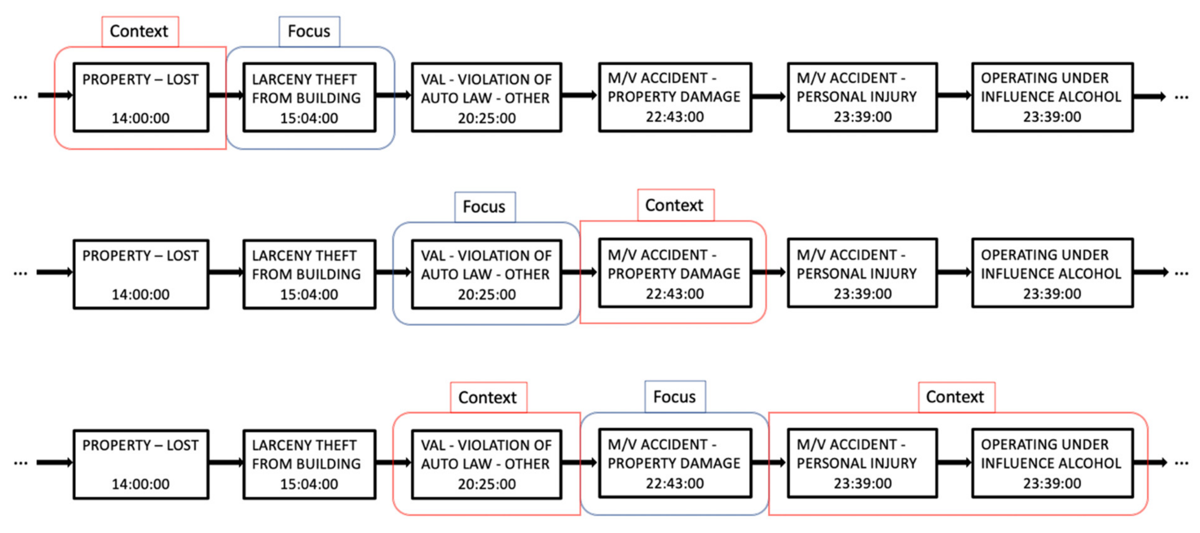
During training, we scan each sequence with a sliding window, identifying, at each step, the current focus crime type and its context, input and target variable to the Skip-gram Word2vec model, respectively. The general statement “crime types are represented according to mutual occurrences in space and time” is, therefore, translated in practice as “crime types are represented according to their time-dependent co-occurrences along space-dependent sequences”. The context of each focus crime type is defined based on the temporal proximity in the same sequence, representing the same spatial area. The temporal proximity is modeled through a time-dependent sliding window, leading to a variable-length context. Unlike traditional Word2vec, setting the model hyperparameter as a chosen fixed number of context elements (e.g., the three previous elements and the three following elements along the sequence), we define the hyperparameter as a chosen time span, therefore leading to a variable number of context elements at each sliding step. For each focus element in the sequence, only the crime types occurring within a certain fixed time span are inserted into the context window. The choice of the time span value is arbitrary, depending on the representation purposes and the time distribution of the crime types; it is particularly influenced by the space resolution hyperparameter, which determines the territory subdivision when building the space-dependent crime sequences. A visual example of the sliding window process is reported in Figure 1, using a context window of three hours in the past and three in the future.
For each focus crime type, the model updates its corresponding embedding vector according to the types falling in its context. By repeatedly performing the auxiliary internal prediction task on the distribution of spatially and temporally contextual crime types, the model ends up with a final embedding representation of the crime types in the “vocabulary”.
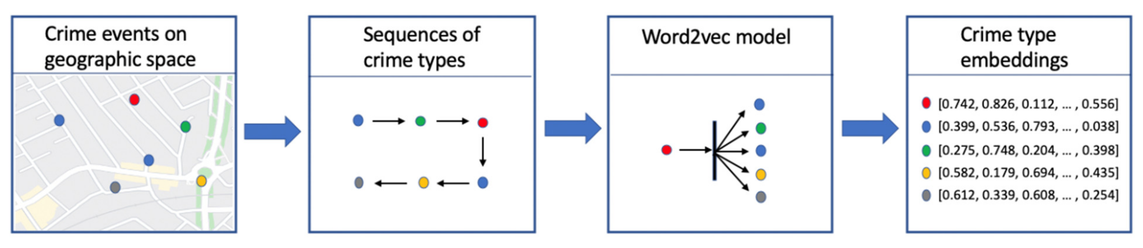
The overall process from raw data to the embedding vectors is summarized in Figure 2.
2.3. Urban Region Vector Space
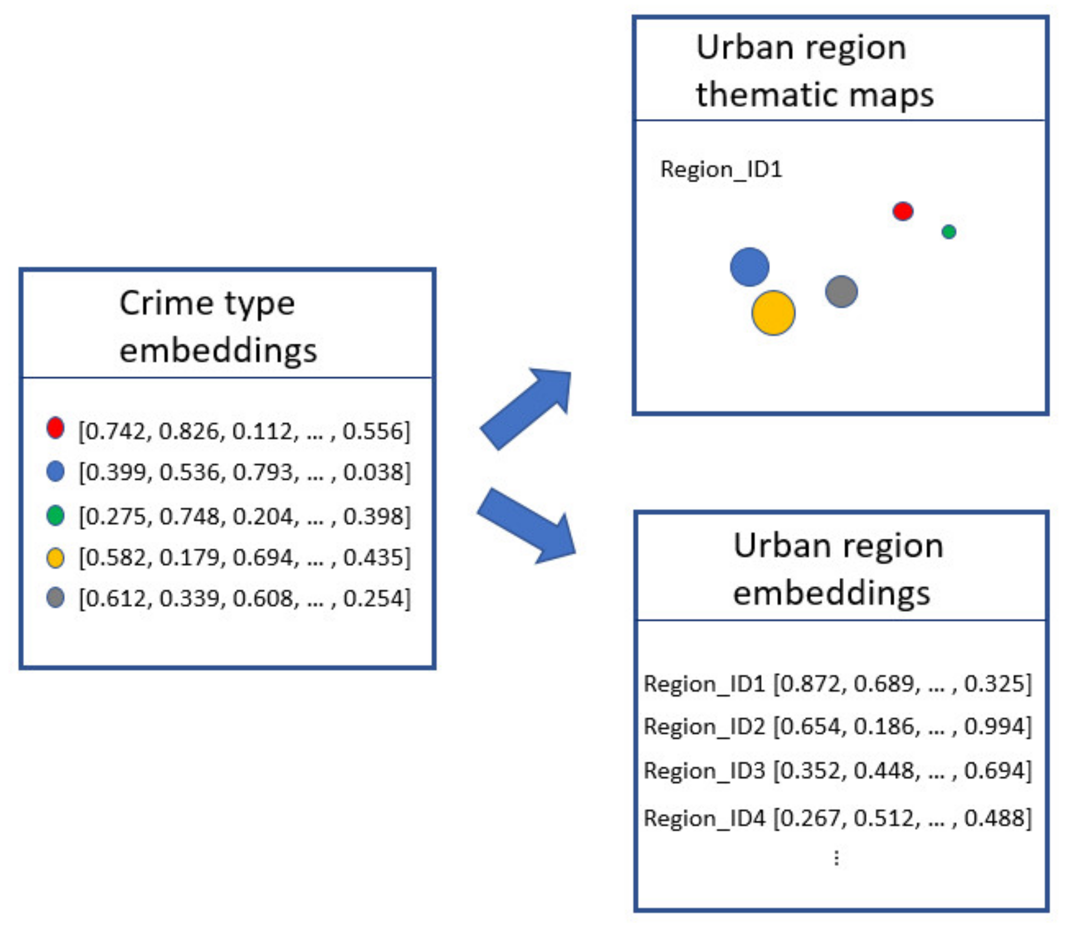
Crime type embeddings can be further utilized for exploring crime type distribution in urban regions. We identified two possible directions, based on the combination of crime type vectors, to deliver information about urban areas. The first direction relies on thematic maps for visualization purposes and intuitive data exploration; the second direction comprises the effective generation of urban region embeddings, allowing for quantitative similarity measures between city areas.
To provide a visually intuitive exploration of crime-related urban regions, we leverage a dimensionally reduced version of the crime type vector space as a template for visualization plots in the form of a thematic map. Inspired by [35], we map the crime type embedding representations into a two-dimensional space and represent the crime configuration of each region as a thematic map adjusted on the crime counts of each type. Since information is aggregated in such semantic space (related crime types are located near each other), the underlying patterns in the crime data are easier to be visually revealed. This can help intuitively understand and conveniently compare crime type distributions across different urban regions.
To quantitatively measure similarities between crime-related urban regions, we create, instead, actual vectors of regions through the combination of crime type vectors. Once the embeddings of single crime types are generated, we use them to obtain dense vectors of urban regions, areas, and portions of territory in general. Particularly, following the simple but effective approach of averaging word embeddings in a text to create document vectors [39,40], we define a crime-related urban region meaning as a composition of individual crime type meanings. The region composition function consists of an average vector over the vectors of all crime elements in the composition:
This bottom-up approach presents the advantage of being efficient, since it reuses already trained models, and effective, as related crime types collectively increase the expression of the corresponding components and, therefore, automatically define distinctive vector characteristics.
Figure 3 summarizes the crime-related urban region analysis.
3. Experiment
This section first describes the selected dataset for training the CrimeVec model and the experimental settings, then reports the results in terms of crime type embeddings, urban region thematic maps, and urban region vectors.
3.1. Data
A real-world crime dataset was used to evaluate the model. The city of Boston (Massachusetts, USA) was selected as a case study, whose crime occurrences and warnings have already been utilized in various research works on crime analysis and prediction [41,42]. Nevertheless, the proposed framework can be applied to any kind of urban territory and sub-territory around the world.
The city of Boston comprises an urban area of 232.14 and a population of 694,583 residents (2018 estimation). The territory is administratively divided into 17 planning districts and 69 neighborhood statistical areas from the Boston Redevelopment Authority, 178 census tracts, 558 census block groups, and 7288 census blocks [43]. Crime data were acquired from the open data portal of the city of Boston (https://data.boston.gov/dataset/crime-incident-reports-august-2015-to-date-source-new-system, accessed on 23 February 2021), officially reporting crime occurrences over the Boston territory. In particular, our case study leverages crime data in the year 2019, registering a total of 93,080 crime events.
Each registered crime event comprises the date and time stamp of occurrence, its geographic location (blurred as the nearest street intersection or centroid between street intersections), and the type of criminal activity. The original crime type categorization is tree-structured, with a higher and lower-level classification. After a process of data cleaning including the removal of unlabeled crime occurrences and very rare crime types, a total of 147 different low-level crime types belonging to 48 top categories were used in the model training. An exemplifying overview of the crime type categorization is reported in Table 1. Due to the geographical distribution of crime occurrences over time, we defined a space resolution for building the input sequences to the embedding model at the level of the census block groups. In general, the choice of parameters such as space resolution and crime type categorization can be defined differently and should be set according to the characteristics of the dataset. Given the selected census block group resolution, a total of 558 possible crime sequences were generated, each of them referring to a unique spatial unit area representing a specific block group.
3.2. Experimental Settings
The CrimeVec model was implemented with a context window size of three hours in the past and three in the future, and a vector size of 25 dimensions. The training process leveraged mini-batch optimization relying on noise-contrastive estimation loss and Adam optimizer [44,45].
To quantify the entity relatedness, we applied the cosine similarity measure to the embedding representations, therefore translating the relational strength of crime types and urban regions into the cosine of the angle between vectors: similarity lowers as the angle grows, while it grows as the angle lessens. The cosine similarity is calculated as the dot product of unit-normalized vectors:
In order to map embeddings into a visually displayable semantic space, we made use of the t-distributed Stochastic Neighbor Embedding (t-SNE) approach [46], whose scope is to reduce dimensionality while trying to keep similar entities close and dissimilar entities apart. Being widely used for visualizing clusters of high-dimensional instances, we adopted it as a means to visually report entity relations in an intuitive way, by mapping 25-dimensional vectors into a two-dimensional semantic space.
3.3. Evaluation
The evaluation findings are organized on two levels: crime types and urban regions.
Crime type evaluation focuses on the vector similarity between single crime types, investigating the direct output of the CrimeVec model. Relatedness of crime types is analyzed, disclosing spatial-temporal inter-category relations concerning the original crime type categorization. On the other hand, urban region evaluation focuses on the result of the compositional approach that combines representations of crime types into representations of urban regions, in the form of qualitative thematic maps obtained through the customization of the crime type vector space, or in the form of actual compositional vectors of urban regions obtained by averaging embeddings of single crime types. We therefore explore the meaning of crime-related similarity of urban areas, and its relationship with geographical proximity.
3.3.1. Crime Type Embeddings
The CrimeVec output is represented by the generation of embedding vectors of single crime types. The comparison of cosine similarities between them describes a network of spatial-temporal relations, revealing information on frequent crime type co-occurrences and, therefore, introducing a new perspective in the analysis of crime type categorizations. High similarity between two different crime types is a sign of high spatial-temporal relatedness, namely frequent occurrences in the same area at the same time span. This leads to grouping crime types in a way that goes beyond the original categorization, typically based on the inherent similarity of the committed crimes from a violation modality perspective. The same top category does not necessarily imply the same spatial-temporal characterization of subtypes, whereas different categories’ crime types can share similar spatial-temporal patterns.
Based on the cosine similarity measures between embeddings vectors, Table 2 reports the top 10 similar types of four reference crime types that serve as an example: “disturbing the peace”, “VAL—operating unregistered/uninsured car”, “weapon—firearm—carrying/possessing”, and “drugs—class B trafficking over 18 g”. The results highlight the captured semantic relations among crime types, indeed revealing intuitively plausible relatedness combinations.
“Disturbing the peace” (belonging to the “disorderly conduct” top category and indicating a conduct that jeopardizes people’s right to peace and tranquility) has a high similarity with crime types related to liquor violations and drug possession. Moreover, it evidences relatedness with a wide variety of different categories, ranging from gathering violation, to harassment, to affray, all of them reasonable connections to peace disturbance in a general sense.
On the other hand, the crime types registering high similarities with “VAL—operating unregistered/uninsured car” (belonging to the top category of “violations”) are mainly car-related, even if not always belonging to the same categorization. For example, “VAL—violation of auto law-other” and “VAL—operating without license” belong to the group of violations of auto law, whereas the other ones (e.g., injuring pedestrians, damaging properties, etc.) are categorized as “motor vehicle accident response”. Few non-car related types are also present, i.e., operating under the influence of alcohol, drug possession, and fugitive from justice. Even in this case, the semantic relatedness of crime embeddings can be justified by a general intuition of plausible spatial-temporal connections.
Regarding “weapon—firearm—carrying/possessing” (belonging to the top category of “firearm violations”), its top similar crimes comprise a substantial variety of categories, involving other weapon-related violations, but also drug possession, auto law violations, and violent crimes such as homicide and aggravated assault. These types are semantically related and can be easily part of the same contextual story (e.g., getting caught carrying firearms when stopped for an auto violation, or trivially possessing weapons when part of an assault or a murder).
Finally, “drugs—class B trafficking over 18 g” (belonging to the top category of “drug violation”), besides being very similar to some other drug violations, turns out to be also strongly connected to weapon-related crimes, suggesting a frequent semantic relationship between trafficking drugs and possessing weapons.
In general, the reported examples point out that crime types belonging to different categories may anyway be strongly related from a spatial-temporal perspective, and consequently ending up being represented as similar vectors, located in the same area of the embedding space. Going beyond the original categorization based on a violation modality point of view, the vector space reveals a complex system of inter-category relations (e.g., relatedness of drug trafficking and weapon possess), and different crime situational perspectives (e.g., peace disturbance as a consequence of liquor or drug violation or as a consequence of a riot or affray). Analyzing similarity measures, we can therefore reveal hidden spatial-temporal patterns in the form of crime relatedness, hence introducing a convenient dynamic data-driven representation of crime types enriching the original standard categorization.
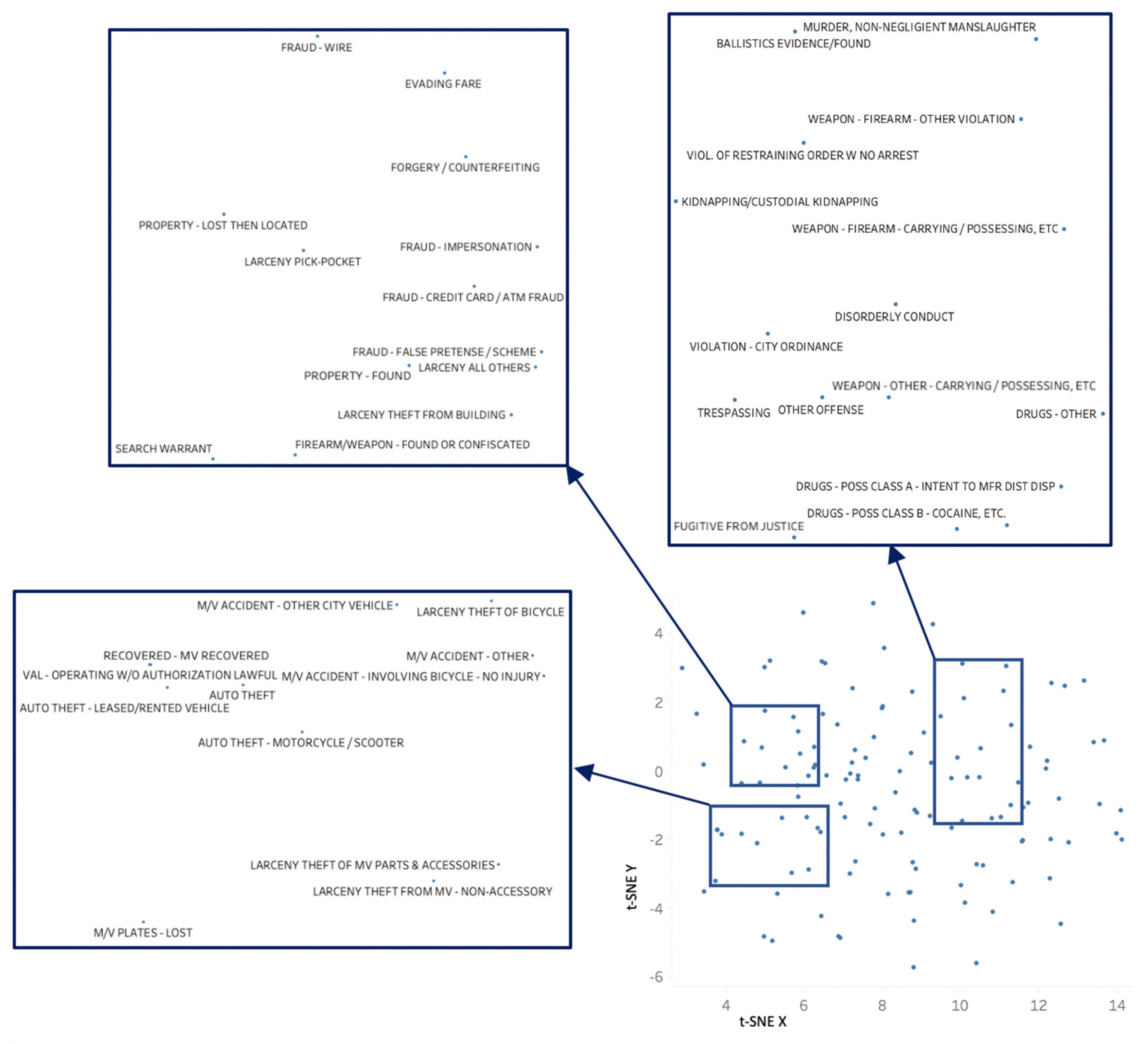
In order to visually represent a global overview of the whole embedding space and the relations between its entities, crime type vectors can be dimensionally reduced through t-SNE and plotted. Figure 4 reports the two-dimensional reduction of the embedding space. A few groups of homogeneous crime types can be noted (e.g., drug possession-related types, motor vehicle accidents), but in general the crime categories are widely mixed up. As a static map does not allow for a clear visualization of all crime type names, the use of an interactive mapping tool (e.g., https://projector.tensorflow.org, accessed on 23 February 2021) is helpful for a better visual investigation of the crime type semantic space through dynamic effects. For a better understanding, three sections of the vector space are enlarged in the reported figure, displaying a mixture of crime types of different nature, reflecting our basic assumption. Specifically, crime types depicted on the lower left mainly comprise motor vehicle accidents and theft-related car violations; crime types on the upper left mostly involve frauds and larcenies; crime types on the upper right refer instead to a wide range of categories including drug violations and weapon-related offenses.
Crime-type frequent co-occurrences in space and time are therefore translated into semantic associations and, consequently, into an index of situational relatedness within a potential context of police perception.
3.3.2. Crime-Related Urban Region Embeddings
The embedding representation of crime types allows for a comparison of urban areas in terms of crime activity relations, therefore not simply based on crime counts, but also considering the collective relatedness of crimes. We developed the comparison strategy following two different methods, a visual qualitative approach and a vector-based quantitative direction. The first one relies on the use of the crime type dimensionally reduced semantic space as a base plot for visualizing crime-related thematic maps of each urban area, a sort of visual fingerprint for an intuitive instant comparison. The second one focuses, instead, on the generation of effective vector representations of single urban regions, allowing for quantitative similarity measures between different geographic areas.
Crime Configuration Plots
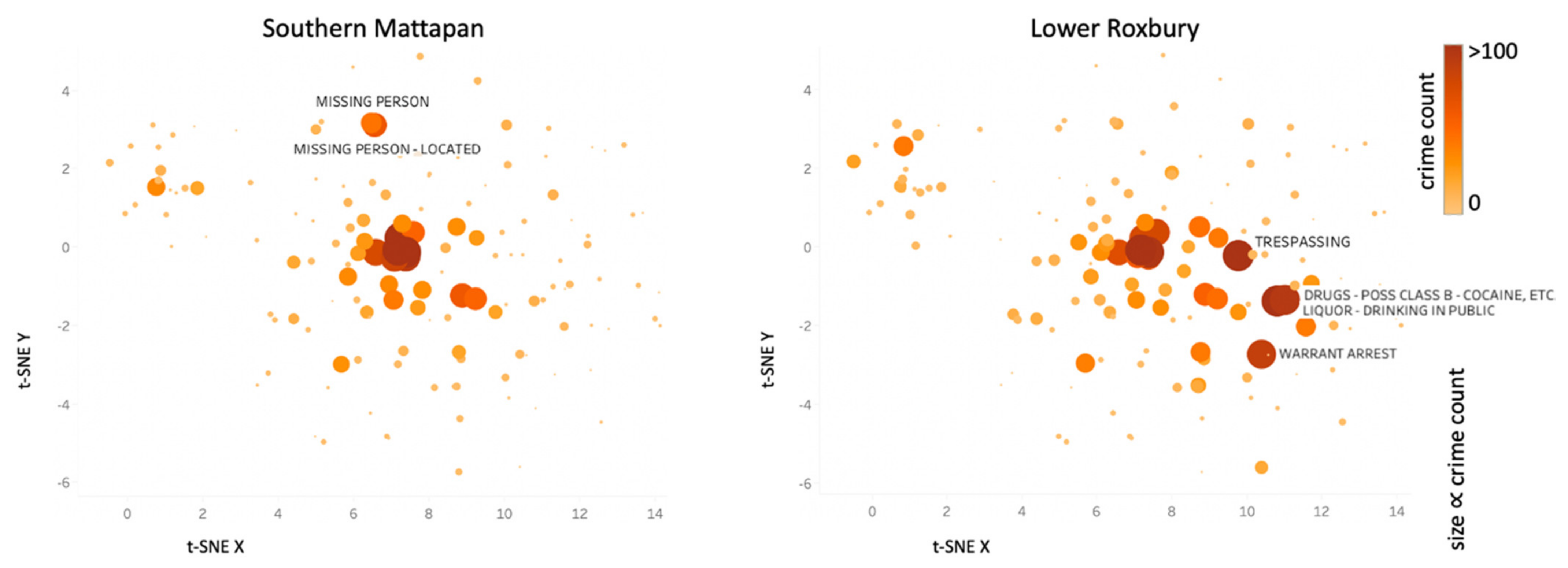
Using the crime type dimensionally reduced vector space as a base map, a visual representation of the crime type semantic distribution of each urban region is defined. The process consists of statistically counting the crime occurrences of the various types, and render the points in the vector space accordingly (e.g., through variable sizes and colors). The whole space representation varies region by region depending on the amount and type distribution of the crime events that occurred in each area. Moreover, as spatial-temporal related crime types are located next to each other in the vector space, information is often clustered on such space, highlighting the underlying patterns and, since the thematic maps are built on the same base map, making the visual comparisons across regions very convenient.
Figure 5 displays the crime type configuration of two urban regions taken as an example, Southern Mattapan and Lower Roxbury. What firstly emerges is the ease in discerning patterns, quickly identifying differences between crime characteristics of individual regions, a distinct advantage over simple statistical tables of crime counts. Indeed, because semantic relations of crime types are learned from their spatial-temporal co-occurrences, the thematic maps tend to report high values of crime counts next to each other, significantly helping to reveal patterns through an appropriate visualization. Comparing the two regions, we observe different configurations between Southern Mattapan and Lower Roxbury. The plot labels immediately reveal some underlying crime information: Southern Mattapan has two prominent overlapping circles identifying the crime types “missing person” and “missing person—located”, disclosing a distinctive crime characteristic in the area; Lower Roxbury identifies instead a higher number of peculiar crime type occurrences, including two overlapping circles representing the crime types “liquor—drinking in public” and “drugs—possession class B—cocaine, etc.”, and other two prominent circles reporting the crime types “trespassing” and “warrant arrest”, identifying a different crime trend featuring further characteristics from the previous one.
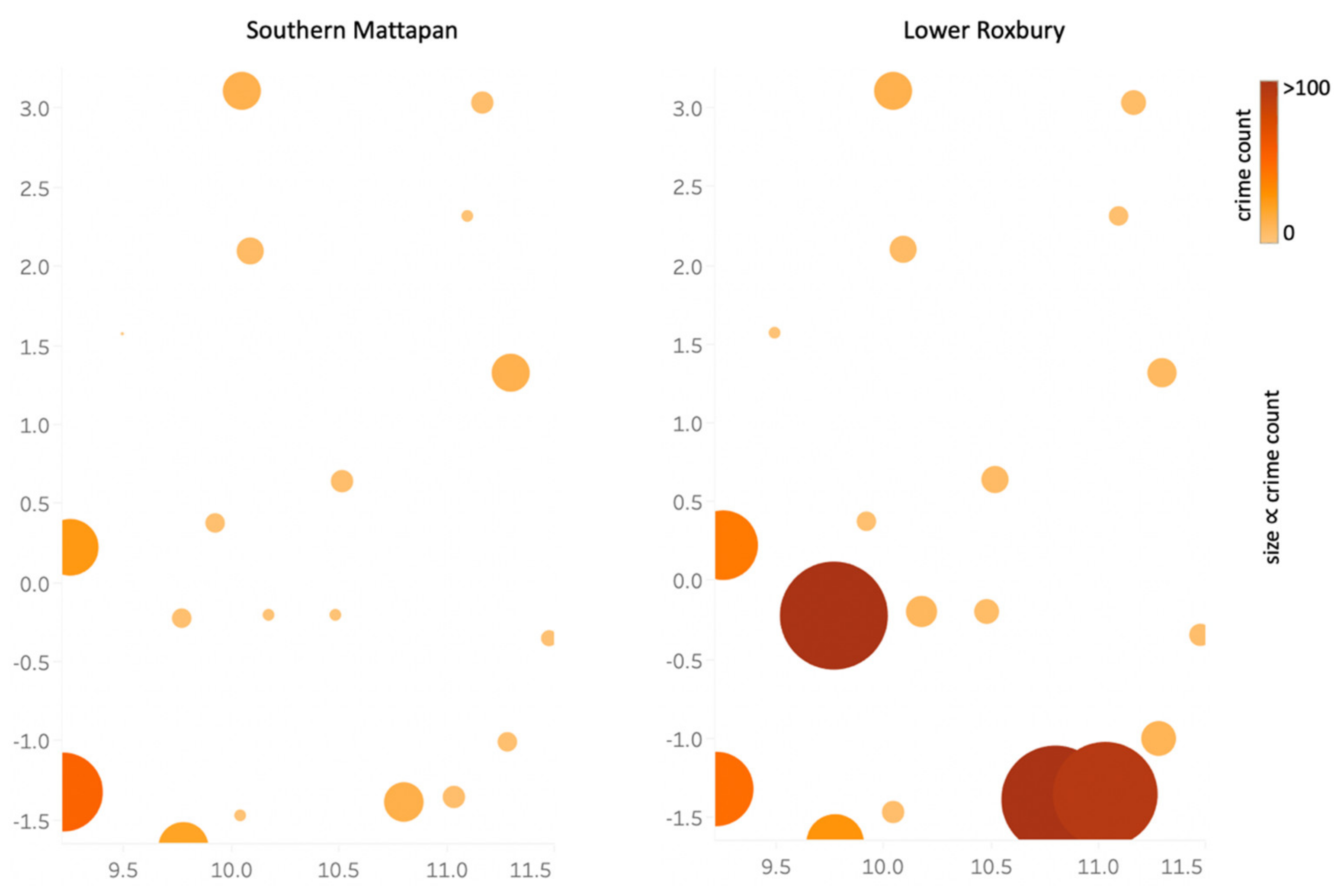
Also, we can focus on a certain vector space section, for example the one reported in the upper right of Figure 4 (mainly defining drug violations and weapon-related offenses), and build the corresponding thematic map for each of the two regions, obtaining the results shown in Figure 6. It emerges that Lower Roxbury has a general tendency of higher numbers of crime occurrences within the selected semantic section. Such visual plots significantly help for a quick understanding of the crime-related urban region characteristics. The use of an interactive tool facilitates the exploration of the thematic maps.
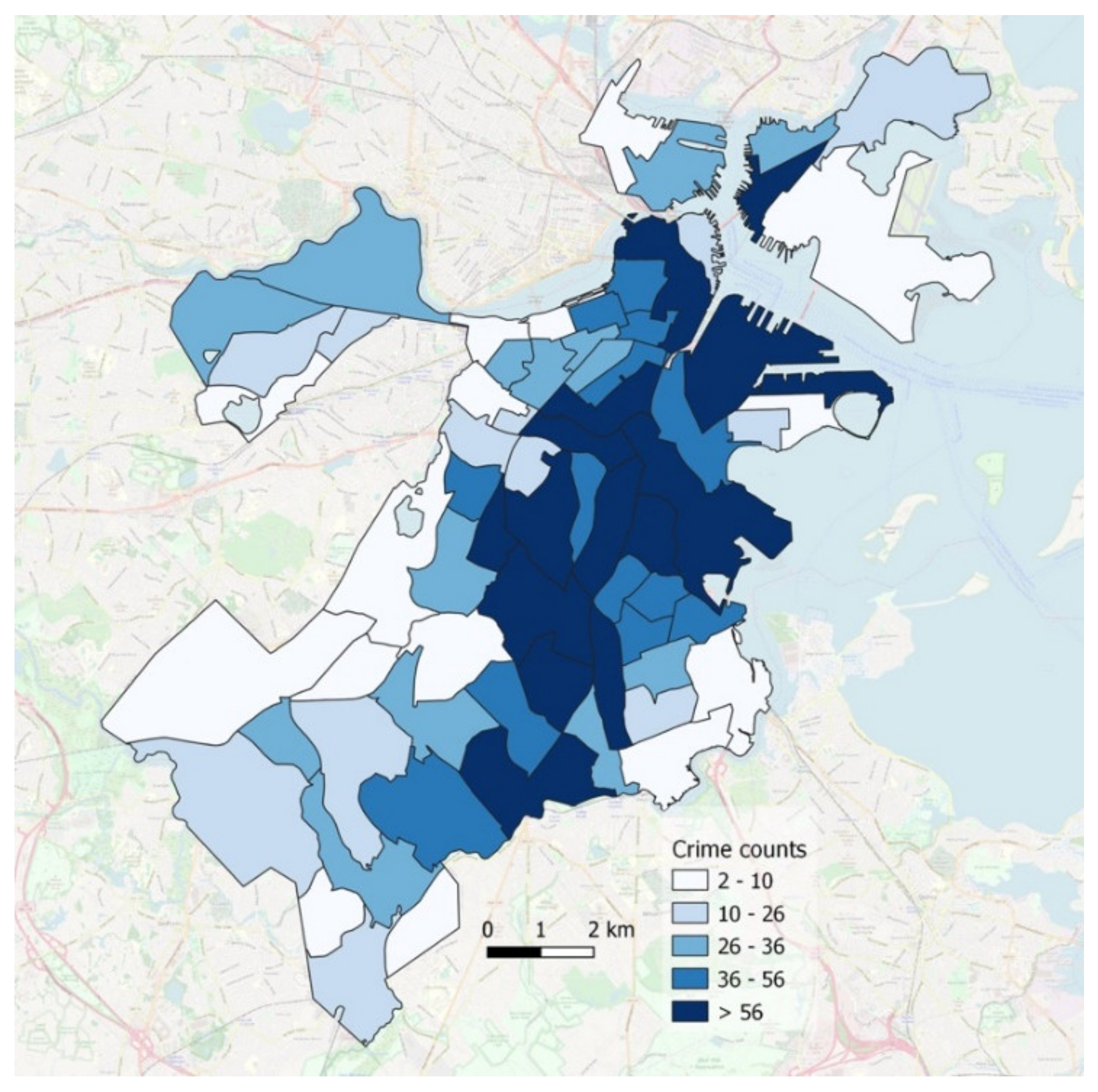
Furthermore, additional analysis can link the semantic space to the geographic space, to spatially analyze crime information across the city. For example, by selecting a group of contiguous crime types in the vector space, we can visualize all urban regions in the geographic space, rendered according to the overall count of the selected types. Since neighboring crime types in the semantic space are related to each other, the group selection identifies a semantic block carrying a specific kind of crime meaning, whose corresponding spatial information is depicted on urban regions across the city. The example of Figure 7 refers to the crime selection in Figure 6, reporting the corresponding geographical information across Boston in terms of the number of occurrences of the crime types within the semantic block. Again, the provided visual tool is a valuable option for intuitively displaying the spatial distribution of semantically related crime types, easily disclosing the influence of chosen semantic blocks over the urban territory.
Urban Region Embeddings
A quantitative similarity-based approach on crime-related urban regions is explored by constructing urban region embeddings as composition vectors of crime type embeddings. The crime pattern relations among urban regions are therefore inherently represented as similarity measures between vectors of geographic areas, obtained by averaging the corresponding embeddings of the registered crime occurrences inside the area (i.e., weighted average of crime types). In this way, crime relatedness between regions was encoded into a single common “urban vector space”.
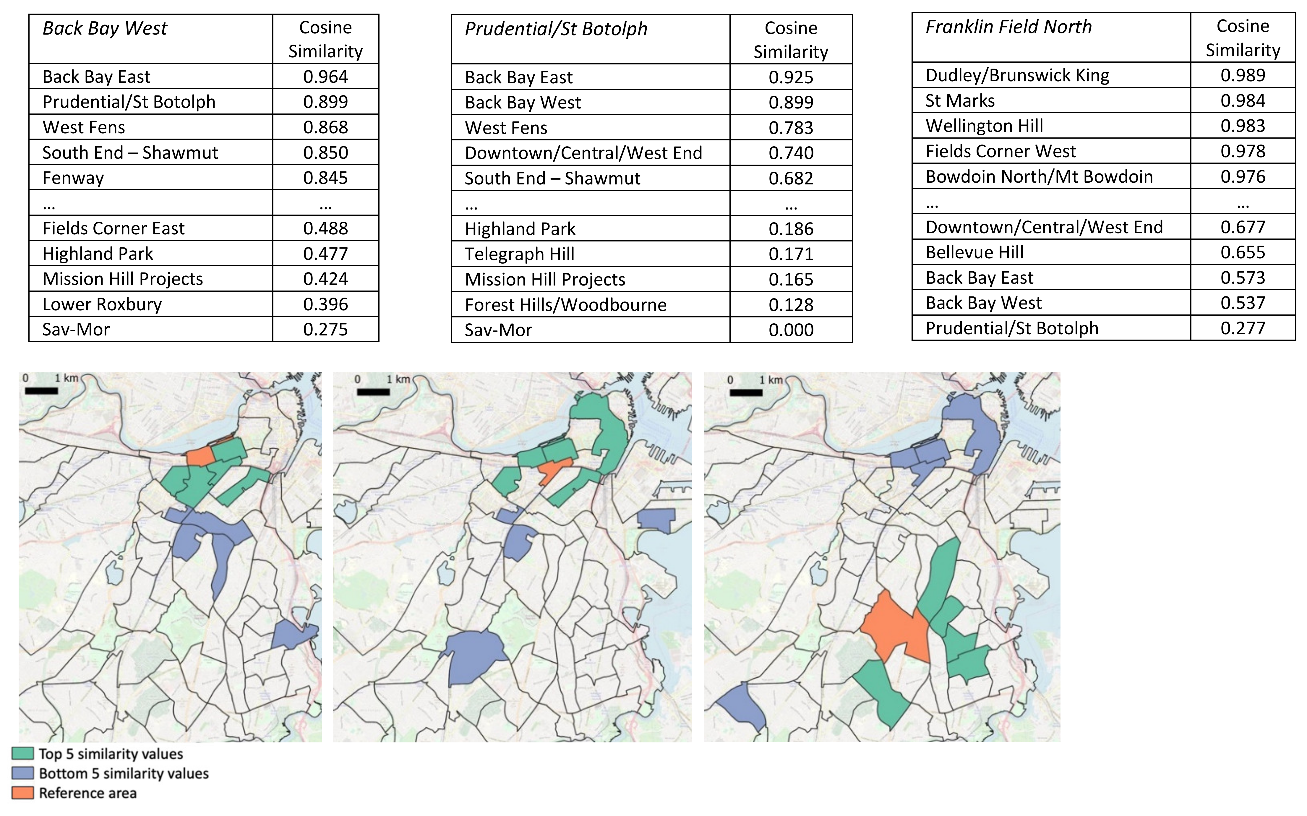
The definition of “urban regions” can refer to any choice of territory division; the approach can be applied for any arbitrarily chosen spatial resolution. To provide a general understanding of the results and facilitate their exposure, we proceeded to divide the territory at the level of Neighborhood Statistical Areas, for a total of 68 urban regions (the 69th area, consisting of the islands in Boston Harbor, was excluded). Figure 8 shows three exemplifying cases reporting the top five and bottom five similar regions of a chosen reference region (the overall similarity distribution was scaled between zero and one), together with their geographic position on the map. At a first look, the crime relatedness between the areas seems to be influenced by their geographical distance to some extent. As a general tendency, this is intuitively explainable when neighboring regions have similar socio-economic and/or functional characteristics, which may determine some kind of influence on the types of committed crimes. However, the link between semantic relatedness and geographic distance is not straightforward, neither in terms of assuming that all neighboring regions share the same characteristics, neither in terms of presuming that those characteristics necessarily affect crime in the same way. Indeed, although a trend is visible in the examples, top and bottom similarities do not distinctly follow strict spatial distance properties (e.g., Franklin Field North top similarities only develop on its eastern and southern sides). Moreover, it is worth noticing how different similarity distributions affect different regions, specifically noting the case of Prudential/St Botolph, which reports much lower top and bottom similarity values compared to the other two cases, therefore, expressing a general weaker tendency of sharing crime patterns with the other regions.
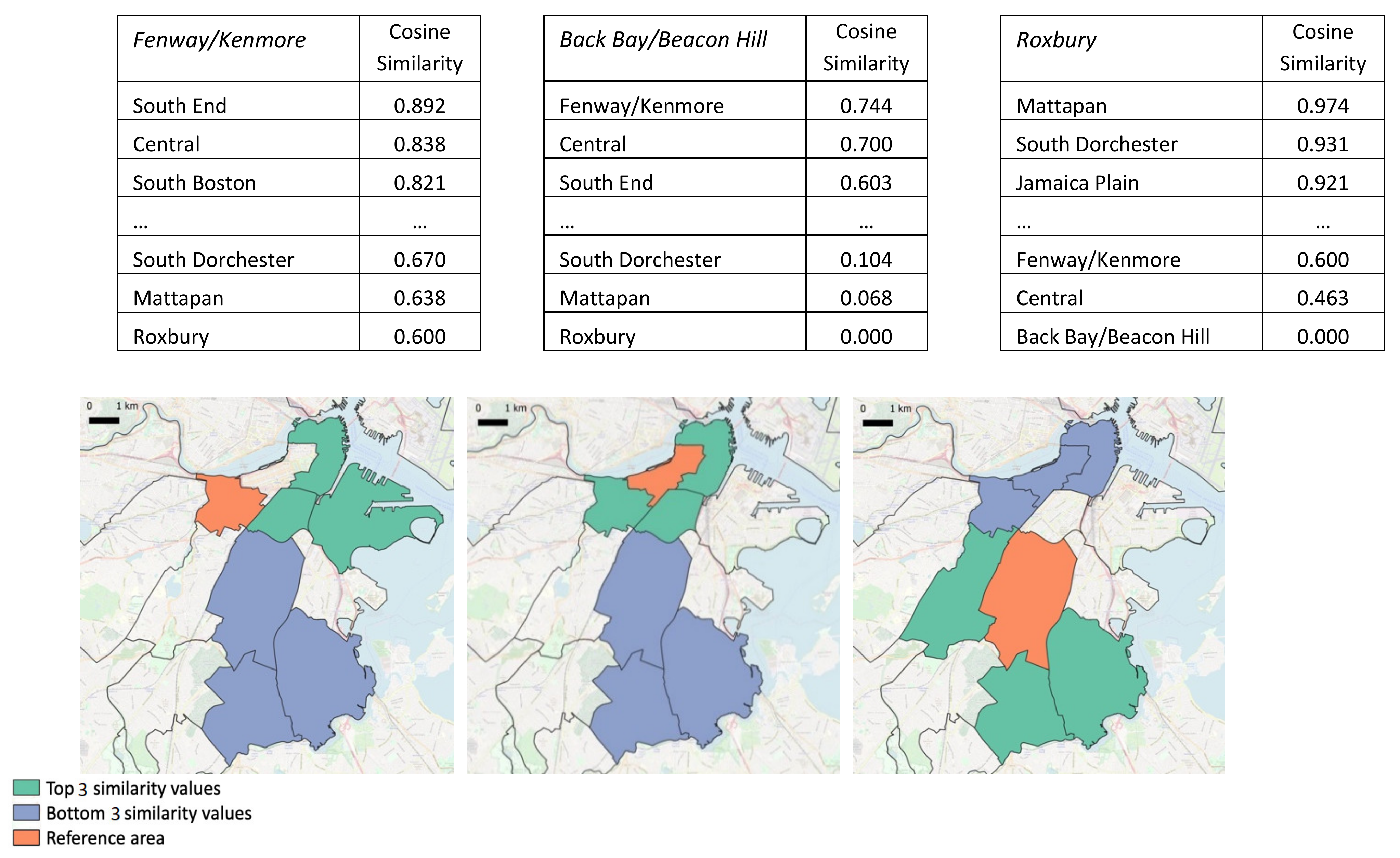
Different space resolutions can be explored when defining the urban regions, even dividing the territory into sections covering larger areas. Figure 9 reports three examples at the level of the 16 planning districts (Harbor Islands were again excluded). As previously noted, the semantic similarity shows a spatial distance influence, even though not strictly (e.g., Fenway/Kenmore case), and the different distribution of similarity values between regions is still observable (e.g., the third most similar region to Back Bay/Beacon Hill has approximately the same score as the least similar region to Fenway/Kenmore).
In addition to the inter-region analysis, intra-region comparisons are also possible. The crime-type occurrences can be gathered in different groups, which in turn can be compared between each other. An option may comprise the study of crime similarities in different hours of the day. Table 3 shows three intra-region examples, at the level of a census tract, reporting the cosine comparisons between morning (6 a.m.–12 p.m.), afternoon (12 p.m.–6 p.m.), evening (6 p.m.–12 a.m.), and night (12 a.m.–6 a.m.), expressions of a stronger or weaker inherent crime relatedness among different portions the day. These particular cases reveal a general trend of disclosing the highest similarity between afternoon and evening while registering the lowest similarity between morning and night.
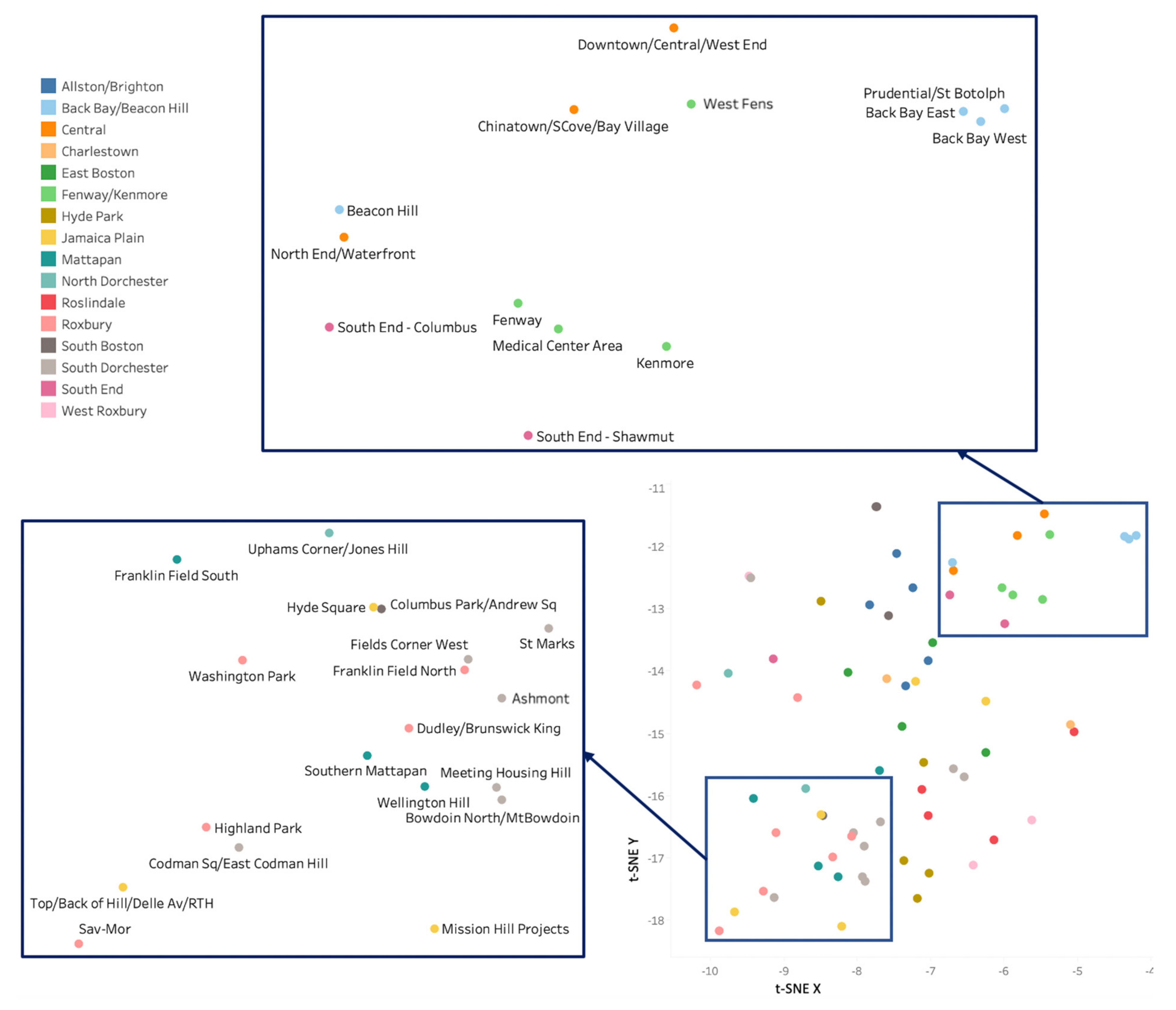
Finally, to have a global overview of the crime relations between the different urban regions, vectors can be dimensionally reduced using t-SNE and plotted. The result is shown in Figure 10, reporting the embeddings of neighborhood statistical areas, whose labels are differently colored based on the planning districts they belong to. The tendency of grouping neighboring regions is clearly observable, but a number of exceptions are also present.
4. Discussion and Conclusions
Crime activity is strongly characterized by spatial and temporal traits, whose investigation is essential in urban policy and city management. Understanding spatial-temporal relations between crime types and urban regions can lead to useful insights on crime patterns and practical views on the functionality and development status of city areas. The traditional approach of making statistics towards the crime counts on separate types neglects the implicit semantic relations between the different types, missing a meaningful aspect of the urban crime configuration. This study proposed a novel framework for exploring implicit semantic relations of crime types and their influence on urban regions’ characterization.
CrimeVec is an approach for creating dense vectors of crime types based on their spatial-temporal distribution, going beyond original crime categorizations by defining an embedding representation solely relying on the way crime types occur in space and time.
The methodology consists of organizing time-stamped geo-located crime events into sequences of crime types that are subsequently fed to an adapted Word2vec model leveraging a time-dependent context window. The output defines the embeddings of crime types by learning their frequent co-occurrences in space and time. Afterward, qualitative thematic plots of single urban regions can be constructed by customizing the dimensionally reduced vector space, and effective embeddings of urban regions can be finally created by combining the vectors of the crime occurrences in each geographic area.
In general, crime type embeddings disclose a complex system of relations, allowing for a direct measure of semantic relatedness. Even though some crime types falling under the same top category have a tendency of ending up close to each other in the vector space (e.g., drug-related crimes), we revealed further relations where crime types belonging to completely different top categories in terms of violation modality determine similar embeddings due to their frequent co-presence in the same areas during the same time span. This process embodies the concept of spatial-temporal similarity into a mathematical representation. The overall idea is indeed to convey similarity measures between a large multitude of different crime types, whereby related crime types will end up assuming similar vector representations, clustering next to each other in the multi-dimensional embedding space, and therefore, implicitly, organizing themselves into higher-level groups in a purely data-driven manner.
Moreover, crime type combinations allow for the exploration of the embedding space at the level of urban regions, helping identify crime-related geographic areas over the territory. This can be firstly done in the form of qualitative thematic maps for intuitively visualizing and conveniently comparing urban regions, making the crime configuration patterns easily discernable. On a more quantitative approach, constructing actual region embeddings defines a comparison mode involving a different implicit meaning than the simple count of crime types inside each area, therefore acquiring a flavor of crime relatedness between regions. While we observed a general tendency for neighboring regions to have similar vector representations, there are several exceptions including areas with comparable spatial distances having different cosine similarities, implying a different crime characterization. Various sizes of urban regions can arbitrarily be explored, and intra-region comparisons are also possible (e.g., crime relatedness over different hours of the day).
To sum up, the main contribution of this study is to provide an effective approach for exploring crime type relatedness and distinctive crime characterizations of urban regions, through machine-readable representations able to convey similarity measures. The proposed model uncovers spatial-temporal relatedness of crime types by identifying which crime events intrinsically share the characteristic of occurring in specific delimited urban areas within similar time spans, leveraging adjustable space-time resolution hyperparameters to accordingly grasp hidden spatial-temporal aspects of the urban reality. We mine the underlying relations of crime types and provide a new perspective of approaching urban crime, disclosing insights on crime semantic relatedness and effectively providing information in the context of urban development and crime-related policy. Embeddings have advantages in meaningfully representing crime types on the basis of their spatial-temporal occurrences, leveraging a methodology that is easily applicable to any arbitrarily wide territory and in the presence of any initial crime categorization. Comparisons of semantically similar crime types can be performed in order to quickly identify the most related types to a given crime type, revealing underlying relations of crime patterns. Furthermore, comparisons of urban regions, either in a visual way or in a score-based metric, uncover interesting associations among city areas, providing a tool for an alternative investigation.
There are several potential extensions of this paper. Specifically, embedding representations can be tested in various applications, either fed into predictive models or used as a basis for clustering approaches and similarity searching. These include comparison and clustering of related crime types and urban regions, pre-processing for machine learning models, analysis of crime relatedness distribution over the territory, and general information delivery on the city areas, potentially merged with further data sources into more complex combinations of data-driven representations. Moreover, various resolutions in time and space can be explored, even leveraging datasets covering different territory sizes (e.g., at the level of a state or a country, or at the level of a city portion or a single neighborhood). Finally, whereas our data-driven model implicitly catches the ensemble outcome of the subtle urban complex aspects that drive space-time relations of crime types, the analysis and reasoning of every single aspect, which are prominently theory-driven, define a future research direction, combining theoretical-based assumptions with data-based evidence.
To conclude, mimicking the use of word embeddings in NLP, which represent a central factor in every task related to meaning, crime embeddings are introduced as significant representations, built on spatial-temporal crime distributions, that can be feasibly used in a variety of crime studies and included in a range of applications dealing with criminal activity data.
Author Contributions
Alessandro Crivellari conceived the conceptual framework; Alessandro Crivellari and Alina Ristea designed the experiments, analyzed the data, and wrote the paper. All authors have read and agreed to the published version of the manuscript.
Funding
This research was funded by the Austrian Science Fund (FWF) through the Doctoral College GIScience at the University of Salzburg (DK W 1237-N23).
Institutional Review Board Statement
Not applicable.
Informed Consent Statement
Not applicable.
Data Availability Statement
The data used in this study are publicly available on the open data portal of the city of Boston (https://data.boston.gov/dataset/crime-incident-reports-august-2015-to-date-source-new-system, accessed on 23 February 2021).
Acknowledgments
Open Access Funding by the Austrian Science Fund (FWF).
Conflicts of Interest
The authors declare no conflict of interest.
References
- Weisburd, D.; Groff, E.R.; Yang, S.-M. The Criminology of Place: Street Segments and Our Understanding of the Crime Problem; Oxford University Press: Oxford, UK, 2012. [Google Scholar]
- Andresen, M.A.; Curman, A.S.; Linning, S.J. The trajectories of crime at places: Understanding the patterns of disaggregated crime types. J. Quant. Criminol. 2017, 33, 427–449. [Google Scholar] [CrossRef] [Green Version]
- Chainey, S.; Tompson, L.; Uhlig, S. The utility of hotspot mapping for predicting spatial patterns of crime. Secur. J. 2008, 21, 4–28. [Google Scholar] [CrossRef]
- Hipp, J.R. Block, tract, and levels of aggregation: Neighborhood structure and crime and disorder as a case in point. Am. Sociol. Rev. 2007, 72, 659–680. [Google Scholar] [CrossRef] [Green Version]
- Bernasco, W. Them again? Same-offender involvement in repeat and near repeat burglaries. Eur. J. Criminol. 2008, 5, 411–431. [Google Scholar] [CrossRef] [Green Version]
- Short, M.B.; D’orsogna, M.R.; Brantingham, P.J.; Tita, G.E. Measuring and modeling repeat and near-repeat burglary effects. J. Quant. Criminol. 2009, 25, 325–339. [Google Scholar] [CrossRef] [Green Version]
- Groff, E. Characterizing the spatio-temporal aspects of routine activities and the geographic distribution of street robbery. In Artificial Crime Analysis Systems: Using Computer Simulations and Geographic Information Systems; IGI Global: Hershey, PA, USA, 2008; pp. 226–251. [Google Scholar]
- Irvin-Erickson, Y. Identifying Risky Places for Crime: An Analysis of the Criminogenic Spatiotemporal Influences of Landscape Features on Street Robberies; Rutgers University-Graduate School-Newark: Newark, NJ, USA, 2014. [Google Scholar]
- Groff, E.; Taniguchi, T. Quantifying crime prevention potential of near-repeat burglary. Police Q. 2019, 22, 330–359. [Google Scholar] [CrossRef]
- Johnson, S.D.; Bernasco, W.; Bowers, K.J.; Elffers, H.; Ratcliffe, J.; Rengert, G.; Townsley, M. Space–time patterns of risk: A cross national assessment of residential burglary victimization. J. Quant. Criminol. 2007, 23, 201–219. [Google Scholar] [CrossRef] [Green Version]
- Piza, E.L.; Carter, J.G. Predicting initiator and near repeat events in spatiotemporal crime patterns: An analysis of residential burglary and motor vehicle theft. Justice Q. 2018, 35, 842–870. [Google Scholar] [CrossRef]
- Kurland, J.; Piza, E. The devil you don’t know: A spatial analysis of crime at Newark’s Prudential Center on hockey game days. J. Sport Saf. Secur. 2018, 3, 1. [Google Scholar]
- Ristea, A.; Andresen, M.A.; Leitner, M. Using tweets to understand changes in the spatial crime distribution for hockey events in Vancouver. Can. Geogr. Géographe Can. 2018, 62, 338–351. [Google Scholar] [CrossRef] [Green Version]
- Kounadi, O.; Ristea, A.; Araujo, A.; Leitner, M. A systematic review on spatial crime forecasting. Crime Sci. 2020, 9, 1–22. [Google Scholar] [CrossRef]
- Malleson, N.; Andresen, M.A. Spatio-temporal crime hotspots and the ambient population. Crime Sci. 2015, 4, 1–8. [Google Scholar] [CrossRef] [Green Version]
- Helbich, M.; Jokar Arsanjani, J. Spatial eigenvector filtering for spatiotemporal crime mapping and spatial crime analysis. Cartogr. Geogr. Inf. Sci. 2015, 42, 134–148. [Google Scholar] [CrossRef]
- Brantingham, P.J. Crime diversity. Criminology 2016, 54, 553–586. [Google Scholar] [CrossRef]
- Kuang, D.; Brantingham, P.J.; Bertozzi, A.L. Crime topic modeling. Crime Sci. 2017, 6, 1–20. [Google Scholar] [CrossRef]
- Grubesic, T.H.; Mack, E.A. Spatio-temporal interaction of urban crime. J. Quant. Criminol. 2008, 24, 285–306. [Google Scholar] [CrossRef]
- Yue, H.; Zhu, X.; Ye, X.; Guo, W. The local colocation patterns of crime and land-use features in Wuhan, China. Isprs Int. J. Geo Inf. 2017, 6, 307. [Google Scholar] [CrossRef] [Green Version]
- Wang, F.; Hu, Y.; Wang, S.; Li, X. Local indicator of colocation quotient with a statistical significance test: Examining spatial association of crime and facilities. Prof. Geogr. 2017, 69, 22–31. [Google Scholar] [CrossRef]
- He, Z.; Deng, M.; Xie, Z.; Wu, L.; Chen, Z.; Pei, T. Discovering the joint influence of urban facilities on crime occurrence using spatial co-location pattern mining. Cities 2020, 99, 102612. [Google Scholar] [CrossRef]
- Pope, M.; Song, W. Spatial relationship and colocation of crimes in Jefferson County, Kentucky. Pap. Appl. Geogr. 2015, 1, 243–250. [Google Scholar] [CrossRef]
- Block, R.L.; Block, C.R. Space, place and crime: Hot spot areas and hot places of liquor-related crime. Crime Place 1995, 4, 145–184. [Google Scholar]
- Farrell, G. Crime concentration theory. Crime Prev. Community Saf. 2015, 17, 233–248. [Google Scholar] [CrossRef]
- Weisburd, D. The law of crime concentration and the criminology of place. Criminology 2015, 53, 133–157. [Google Scholar] [CrossRef]
- Bengio, Y.; Ducharme, R.; Vincent, P.; Janvin, C. A neural probabilistic language model. J. Mach. Learn. Res. 2003, 3, 1137–1155. [Google Scholar]
- Mikolov, T.; Chen, K.; Corrado, G.; Dean, J. Efficient estimation of word representations in vector space. arXiv 2013, arXiv:1301.3781. [Google Scholar]
- Mikolov, T.; Sutskever, I.; Chen, K.; Corrado, G.; Dean, J. Distributed representations of words and phrases and their compositionality. arXiv 2013, arXiv:1301.3781. [Google Scholar]
- Pennington, J.; Socher, R.; Manning, C.D. Glove: Global Vectors for Word Representation. In Proceedings of the 2014 Conference on Empirical Methods in Natural Language Processing (EMNLP), Doha, Qatar, 25–29 October 2014; pp. 1532–1543. [Google Scholar]
- Liu, X.; Andris, C.; Rahimi, S. Place niche and its regional variability: Measuring spatial context patterns for points of interest with representation learning. Comput. Environ. Urban. Syst. 2019, 75, 146–160. [Google Scholar] [CrossRef]
- Qiu, P.; Gao, J.; Yu, L.; Lu, F. Knowledge embedding with geospatial distance restriction for geographic knowledge graph completion. Isprs Int. J. Geo-Inf. 2019, 8, 254. [Google Scholar] [CrossRef] [Green Version]
- Yao, Y.; Li, X.; Liu, X.; Liu, P.; Liang, Z.; Zhang, J.; Mai, K. Sensing spatial distribution of urban land use by integrating points-of-interest and Google word2vec model. Int. J. Geogr. Inf. Sci. 2017, 31, 825–848. [Google Scholar] [CrossRef]
- Zhai, W.; Bai, X.; Shi, Y.; Han, Y.; Peng, Z.-R.; Gu, C. Beyond word2vec: An approach for urban functional region extraction and identification by combining place2vec and pois. Comput. Environ. Urban. Syst. 2019, 74, 1–12. [Google Scholar] [CrossRef]
- Liu, K.; Yin, L.; Lu, F.; Mou, N. Visualizing and exploring poi configurations of urban regions on poi-type semantic space. Cities 2020, 99, 102610. [Google Scholar] [CrossRef]
- Yan, B.; Janowicz, K.; Mai, G.; Gao, S. From Itdl to Place2vec: Reasoning About Place Type Similarity and Relatedness by Learning Embeddings from Augmented Spatial Contexts. In Proceedings of the 25th ACM SIGSPATIAL International Conference on Advances in Geographic Information Systems, Redondo Beach, CA, USA, 7–10 November 2017; pp. 1–10. [Google Scholar]
- Crivellari, A.; Beinat, E. From motion activity to geo-embeddings: Generating and exploring vector representations of locations, traces and visitors through large-scale mobility data. Isprs Int. J. Geo Inf. 2019, 8, 134. [Google Scholar] [CrossRef] [Green Version]
- Zhou, Z.; Meng, L.; Tang, C.; Zhao, Y.; Guo, Z.; Hu, M.; Chen, W. Visual abstraction of large scale geospatial origin-destination movement data. Ieee Trans. Vis. Comput. Graph. 2018, 25, 43–53. [Google Scholar] [CrossRef]
- Kutuzov, A.; Kopotev, M.; Sviridenko, T.; Ivanova, L. Clustering comparable corpora of Russian and Ukrainian academic texts: Word embeddings and semantic fingerprints. arXiv 2016, arXiv:1604.05372. [Google Scholar]
- Wieting, J.; Bansal, M.; Gimpel, K.; Livescu, K. Towards universal paraphrastic sentence embeddings. arXiv 2015, arXiv:1301.3781. [Google Scholar]
- O’Brien, D.T.; Winship, C. The gains of greater granularity: The presence and persistence of problem properties in urban neighborhoods. J. Quant. Criminol. 2017, 33, 649–674. [Google Scholar] [CrossRef]
- Sommer, A.J.; Lee, M.; Bind, M.-A.C. Comparing apples to apples: An environmental criminology analysis of the effects of heat and rain on violent crimes in Boston. Palgrave Commun. 2018, 4, 1–10. [Google Scholar] [CrossRef]
- O’Brien, D.T.; Phillips, N.E.; Sheini, S.; de Benedictis-Kessner, J.; Ristea, A.; Tucker, R. Geographical Infrastructure for the City of Boston v. 2019; Harvard Dataverse: Cambridge, MA, USA, 2019. [Google Scholar]
- Kingma, D.P.; Ba, J. Adam: A method for stochastic optimization. arXiv 2014, arXiv:1301.3781. [Google Scholar]
- Mnih, A.; Kavukcuoglu, K. Learning word embeddings efficiently with noise-contrastive estimation. Adv. Neural Inf. Process. Syst. 2013, 26, 2265–2273. [Google Scholar]
- Van der Maaten, L.; Hinton, G. Visualizing data using t-sne. J. Mach. Learn. Res. 2008, 9, 11. [Google Scholar]
Figure 1.
Sliding window process with a context window of three hours in the past and three in the future.
Figure 1.
Sliding window process with a context window of three hours in the past and three in the future.

Figure 2.
CrimeVec overall framework.

Figure 3.
Urban region analysis framework.

Figure 4.
Dimensionally reduced crime type vector space.

Figure 5.
Exemplifying thematic maps of Southern Mattapan and Lower Roxbury.

Figure 6.
Exemplifying section of the thematic maps of Southern Mattapan and Lower Roxbury.

Figure 7.
Geographic distribution of crime events within the selected semantic block of Figure 6.
Figure 7.
Geographic distribution of crime events within the selected semantic block of Figure 6.

Figure 8.
Top five and bottom five similar regions of three selected reference regions (neighborhood statistical areas).
Figure 8.
Top five and bottom five similar regions of three selected reference regions (neighborhood statistical areas).

Figure 9.
Top three and bottom three similar regions of three selected reference regions (planning districts).
Figure 9.
Top three and bottom three similar regions of three selected reference regions (planning districts).

Figure 10.
Dimensionally reduced vector space of crime-related regions.


Table 1.
Exemplifying summary of the original crime type categorization.
| Top Categories | Lower-Level Types |
|---|---|
| Drug Violation | Drugs—sale/manufacturing Drugs—class A trafficking over 18 g Drugs—sick assist—heroin … |
| Larceny | Larceny theft from building Larceny shoplifting Larceny pickpocket … |
| Motor Vehicle Accident Response | M/V—leaving scene—personal injury M/V accident—police vehicle M/V—leaving scene—property damage … |
| Violations | VAL—operating without license VAL—operating after revision/suspension VAL—operating unregistered/uninsured car … |
| … | … |
Table 2.
Top 10 similar types of four selected reference crime types.
| Disturbing the Peace | Cosine Similarity |
|---|---|
| Liquor law violation | 0.705 |
| Drugs—possession class D | 0.625 |
| Disorderly conduct | 0.609 |
| Other offense | 0.589 |
| Liquor—drinking in public | 0.574 |
| Drugs—possession class D—intent to distribute | 0.543 |
| Demonstration/riot | 0.517 |
| Affray | 0.516 |
| Evading fare | 0.507 |
| Harassment | 0.5 |
| VAL—Operating Unregistered/Uninsured Car | Cosine Similarity |
| VAL—violation of auto law—other | 0.745 |
| M/V accident involving pedestrian—injury | 0.687 |
| VAL—operating without license | 0.653 |
| Operating under the influence alcohol | 0.642 |
| Stolen property—buying/receiving/possessing | 0.633 |
| M/V accident—involving bicycle—no injury | 0.615 |
| M/V accident—property damage | 0.601 |
| Drugs—possession class D—intent to distribute | 0.596 |
| Fugitive from justice | 0.58 |
| M/V accident—personal injury | 0.574 |
| Weapon—Firearm—Carrying/possessing, etc. | Cosine Similarity |
| Weapon—other—other violation | 0.645 |
| Weapon—other—carrying/possessing, etc. | 0.628 |
| Drugs—possession class B—intent to distribute | 0.597 |
| Weapon—firearm—other violation | 0.596 |
| VAL—violation of auto law—other | 0.587 |
| Murder, non-negligent manslaughter | 0.573 |
| VAL—operating unregistered/uninsured car | 0.564 |
| Assault—aggravated—battery | 0.563 |
| Ballistics evidence/found | 0.561 |
| Drugs—possession class A—intent to distribute | 0.546 |
| Drugs—Class B Trafficking over 18 Grams | Cosine Similarity |
| Drugs—possession class A—intent to distribute | 0.657 |
| Drugs—possession class B—intent to distribute | 0.629 |
| Weapon—other—other violation | 0.566 |
| Drugs—class A trafficking over 18 g | 0.544 |
| Ballistics evidence/found | 0.524 |
| Drugs—possession class B—cocaine, etc. | 0.511 |
| Weapon—firearm—other violation | 0.509 |
| Obscene materials—pornography | 0.502 |
| Search warrant | 0.499 |
| Weapon—firearm—carrying/possessing, etc. | 0.492 |
Table 3.
Example of intra-region similarity comparisons based on different time portions of the day.
Table 3.
Example of intra-region similarity comparisons based on different time portions of the day.
| Beacon Hill | Cosine Similarity | City Point | Cosine Similarity | Jeffrey Point/Airport | Cosine Similarity |
|---|---|---|---|---|---|
| Morning vs. Afternoon | 0.899 | Morning vs. Afternoon | 0.94 | Morning vs. Afternoon | 0.912 |
| Afternoon vs. Evening | 0.99 | Afternoon vs. Evening | 0.989 | Afternoon vs. Evening | 0.985 |
| Evening vs. Night | 0.984 | Evening vs. Night | 0.968 | Evening vs. Night | 0.969 |
| Night vs. Morning | 0.878 | Night vs. Morning | 0.871 | Night vs. Morning | 0.875 |
| Morning vs. Evening | 0.878 | Morning vs. Evening | 0.955 | Morning vs. Evening | 0.886 |
| Afternoon vs. Night | 0.976 | Afternoon vs. Night | 0.964 | Afternoon vs. Night | 0.974 |
Publisher’s Note: MDPI stays neutral with regard to jurisdictional claims in published maps and institutional affiliations. |
© 2021 by the authors. Licensee MDPI, Basel, Switzerland. This article is an open access article distributed under the terms and conditions of the Creative Commons Attribution (CC BY) license (https://creativecommons.org/licenses/by/4.0/).
Share and Cite
MDPI and ACS Style
Crivellari, A.; Ristea, A. CrimeVec—Exploring Spatial-Temporal Based Vector Representations of Urban Crime Types and Crime-Related Urban Regions. ISPRS Int. J. Geo-Inf. 2021, 10, 210. https://doi.org/10.3390/ijgi10040210
AMA Style
Crivellari A, Ristea A. CrimeVec—Exploring Spatial-Temporal Based Vector Representations of Urban Crime Types and Crime-Related Urban Regions. ISPRS International Journal of Geo-Information. 2021; 10(4):210. https://doi.org/10.3390/ijgi10040210
Chicago/Turabian StyleCrivellari, Alessandro, and Alina Ristea. 2021. "CrimeVec—Exploring Spatial-Temporal Based Vector Representations of Urban Crime Types and Crime-Related Urban Regions" ISPRS International Journal of Geo-Information 10, no. 4: 210. https://doi.org/10.3390/ijgi10040210
Note that from the first issue of 2016, this journal uses article numbers instead of page numbers. See further details here.