
Improved Indoor Positioning by Means of Occupancy Grid Maps Automatically Generated from OSM Indoor Data


Abstract
:1. Introduction
2. Related Work
2.1. Positioning
2.2. Occupancy Grid Maps
3. Methodology
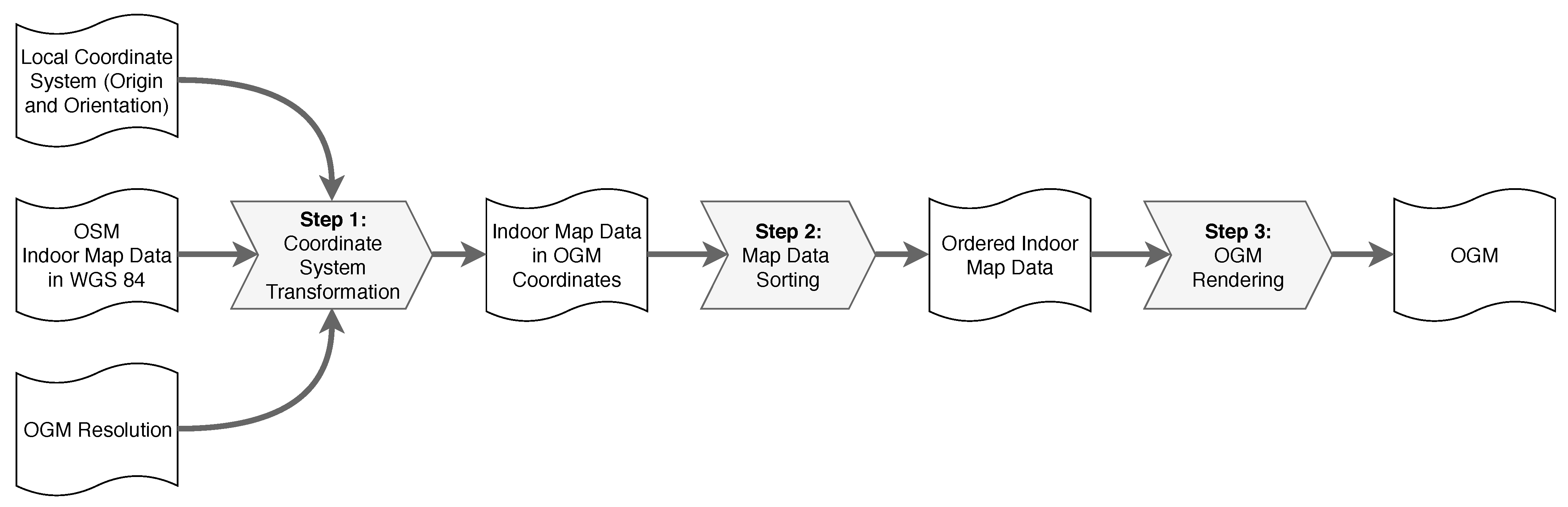
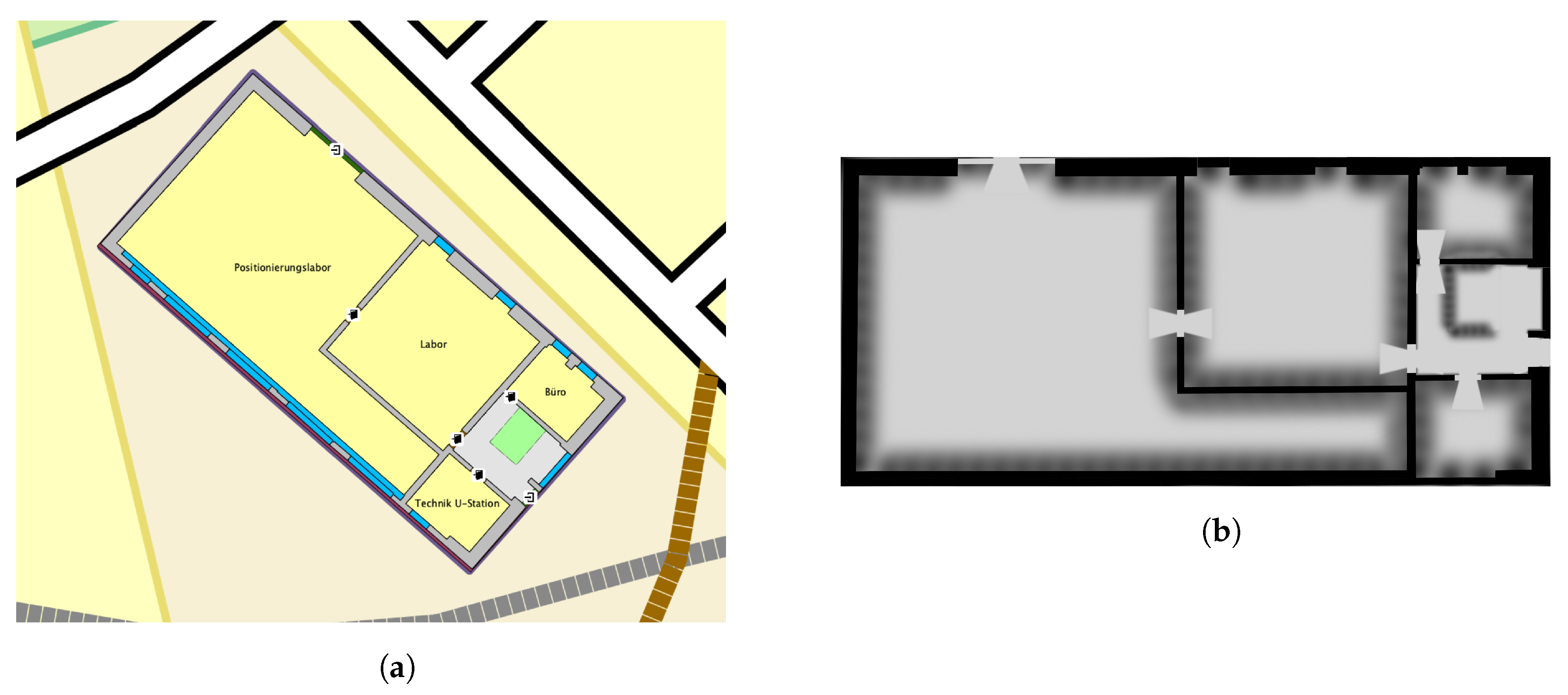
3.1. Automated OGM Generation
3.1.1. Input Data
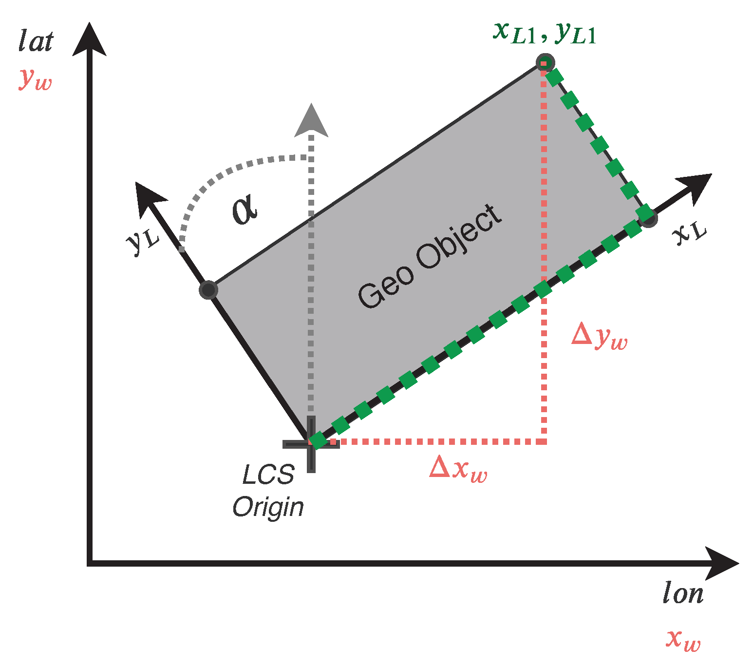
3.1.2. Step 1: Coordinate System Transformation
| Algorithm 1: Algorithm to calculate local metric distances ( and ) between each indoor coordinate and the origin of the LCS. |
 |
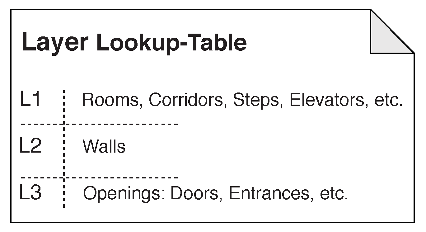
3.1.3. Step 2: Map Data Sorting
3.1.4. Step 3: OGM Rendering
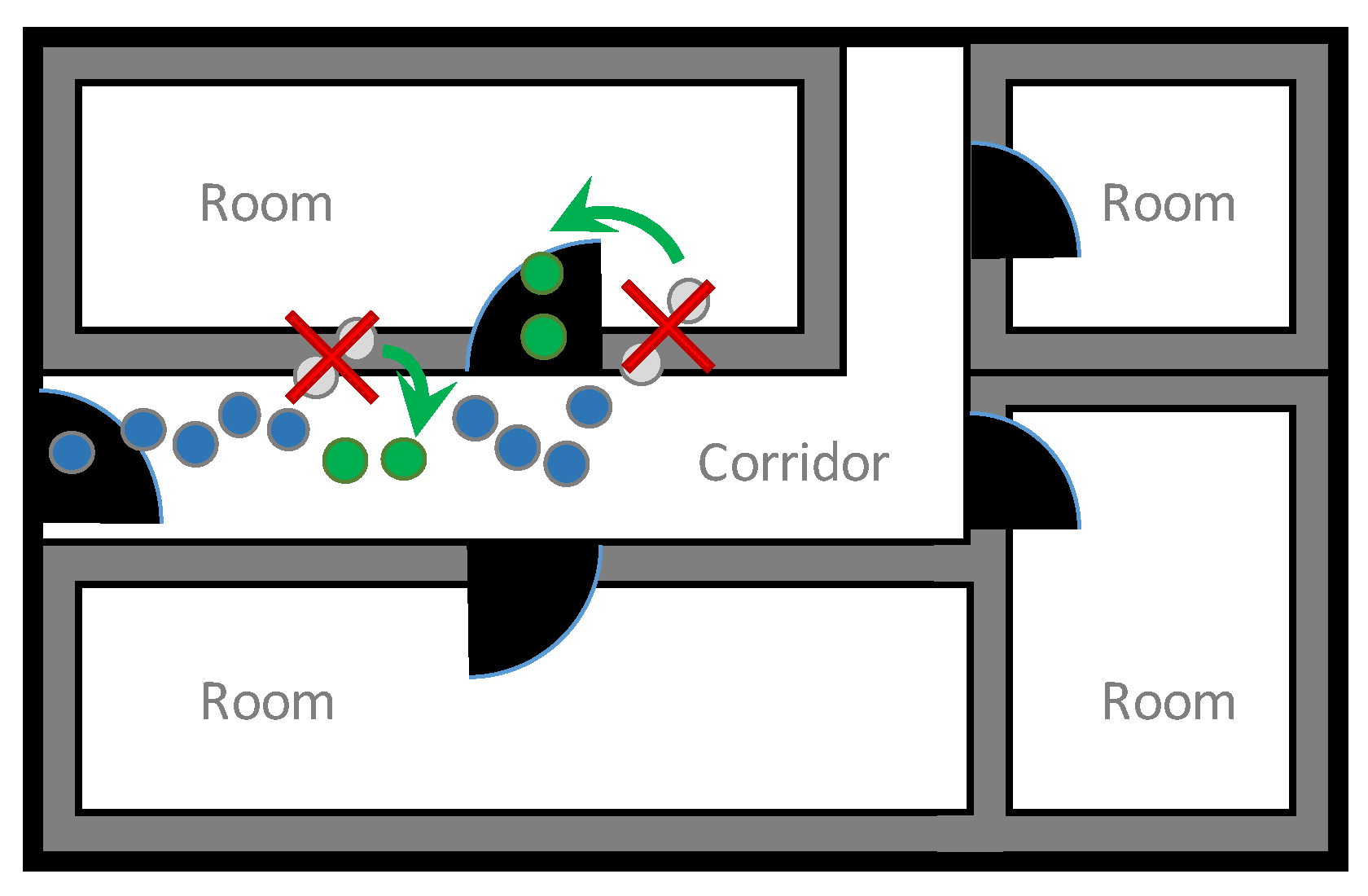
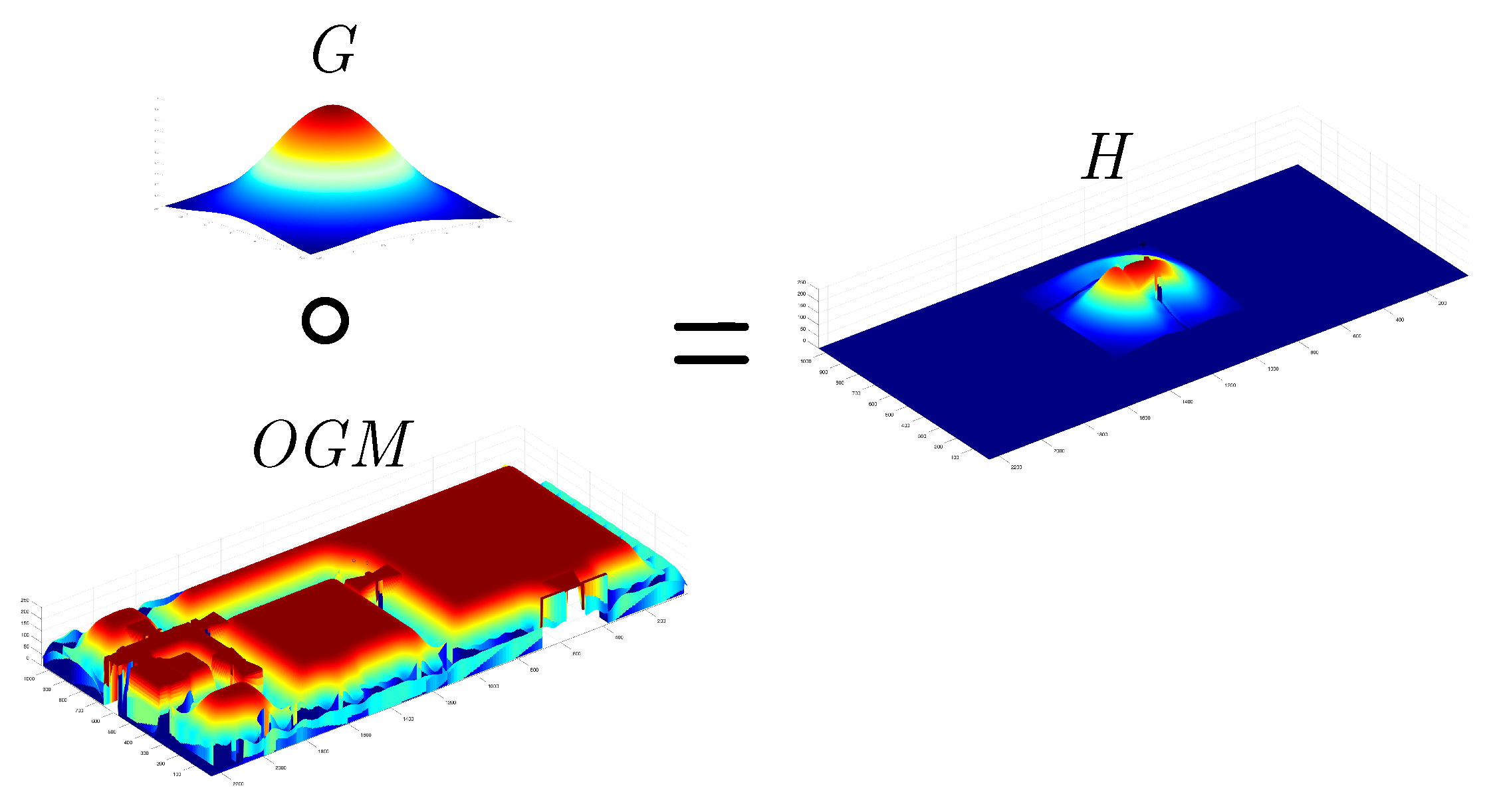
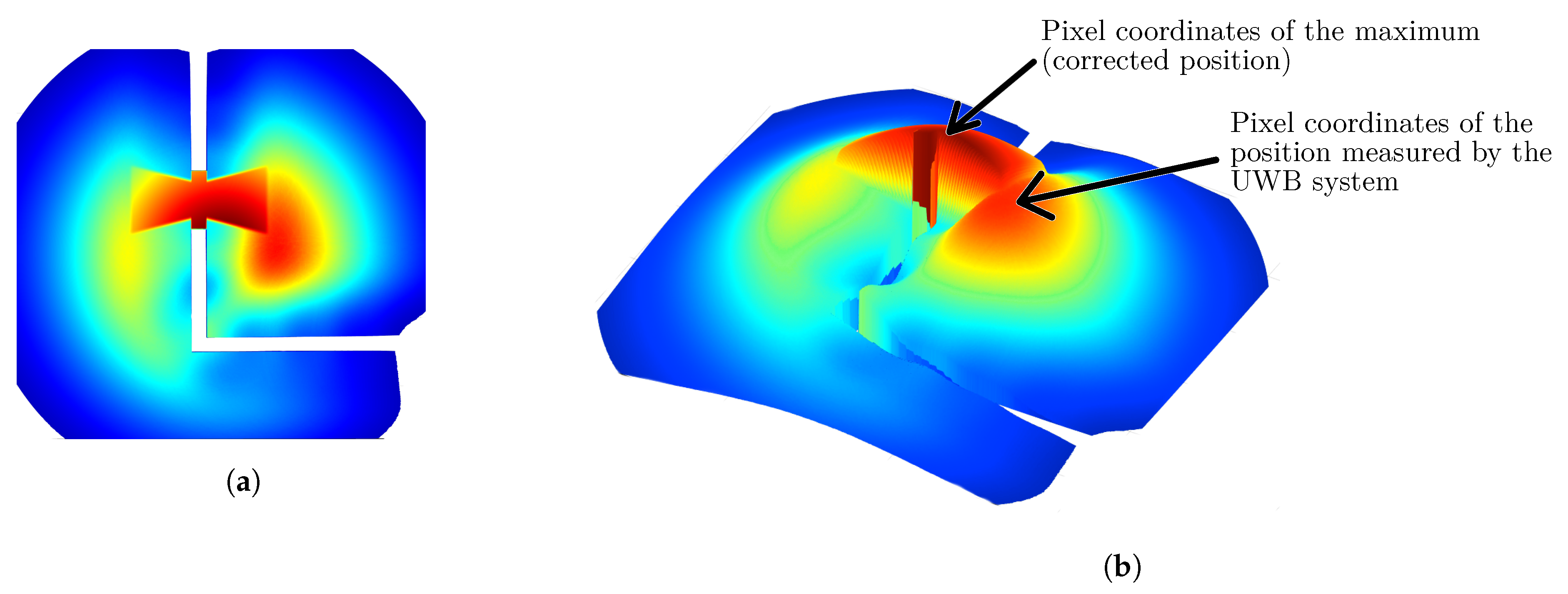
3.2. Positioning Improvement
3.2.1. Method
3.2.2. Gaussian Mask Parameters
4. Results and Discussion
4.1. OGM Generation
4.2. Positioning Improvement
5. Conclusions and Future Work
5.1. OGM Generation
5.2. Positioning Improvement
Author Contributions
Funding
Institutional Review Board Statement
Informed Consent Statement
Conflicts of Interest
References
- Caron, C.; Chamberland-Tremblay, D.; Lapierre, C.; Hadaya, P.; Roche, S.; Saada, M. Indoor Positioning. In Encyclopedia of GIS; Shekhar, S., Xiong, H., Zhou, X., Eds.; Springer: Cham, Switzerland, 2017; pp. 1011–1019. [Google Scholar] [CrossRef]
- Brena, R.F.; García-Vázquez, J.P.; Galván-Tejada, C.E.; Muñoz-Rodriguez, D.; Vargas-Rosales, C.; Fangmeyer, J. Evolution of Indoor Positioning Technologies: A Survey. J. Sens. 2017, 2017, 2630413. [Google Scholar] [CrossRef]
- Link, J.A.B.; Smith, P.; Viol, N.; Wehrle, K. FootPath: Accurate Map-Based Indoor Navigation Using Smartphones. In Proceedings of the 2011 International Conference on Indoor Positioning and Indoor Navigation, Guimarães, Portugal, 21–23 September 2011; pp. 1–8. [Google Scholar] [CrossRef] [Green Version]
- Ramadhan, H.; Yustiawan, Y.; Kwon, J. Applying Movement Constraints to BLE RSSI-Based Indoor Positioning for Extracting Valid Semantic Trajectories. Sensors 2020, 20, 527. [Google Scholar] [CrossRef] [PubMed] [Green Version]
- Kokkinis, A.; Raspopoulos, M.; Kanaris, L.; Liotta, A.; Stavrou, S. Map-Aided Fingerprint-Based Indoor Positioning. In Proceedings of the 2013 IEEE 24th Annual International Symposium on Personal, Indoor, and Mobile Radio Communications (PIMRC), London, UK, 8–11 September 2013; pp. 270–274. [Google Scholar] [CrossRef]
- Meng, J.; Ren, M.; Wang, P.; Zhang, J.; Mou, Y. Improving Positioning Accuracy via Map Matching Algorithm for Visual–Inertial Odometer. Sensors 2020, 20, 552. [Google Scholar] [CrossRef] [PubMed] [Green Version]
- Consortium, O.G. CityGML | OGC. 2021. Available online: https://www.ogc.org/standards/citygml (accessed on 5 March 2021).
- Consortium, O.G. IndoorGML | OGC. 2021. Available online: https://www.ogc.org/standards/indoorgml (accessed on 5 March 2021).
- Poljansek, M. Building Information Modelling (BIM) Standardization. 2018. Available online: https://ec.europa.eu/jrc/en/publication/building-information-modelling-bim-standardization (accessed on 5 March 2021).
- OSM-Community. Simple Indoor Tagging–OpenStreetMap Wiki. 2021. Available online: https://wiki.openstreetmap.org/wiki/Simple_Indoor_Tagging (accessed on 5 March 2021).
- Li, K.J.; Conti, G.; Konstantinidis, E.; Zlatanova, S.; Bamidis, P. 10-OGC IndoorGML: A Standard Approach for Indoor Maps. In Geographical and Fingerprinting Data to Create Systems for Indoor Positioning and Indoor/Outdoor Navigation; Conesa, J., Pérez-Navarro, A., Torres-Sospedra, J., Montoliu, R., Eds.; Intelligent Data-Centric Systems, Academic Press: Cambridge, MA, USA, 2019; pp. 187–207. [Google Scholar] [CrossRef]
- Topf, J. OpenStreetMap Taginfo | Tags | Indoor=room. Available online: https://taginfo.openstreetmap.org/tags/indoor=room (accessed on 5 March 2021).
- OSM-Community. Indoor Mapping–OpenStreetMap Wiki. 2020. Available online: https://wiki.openstreetmap.org/wiki/Indoor_Mapping (accessed on 5 March 2021).
- Graichen, T.; Schmidt, R.; Richter, J.; Heinkel, U. Occupancy Grid Map Generation from OSM Indoor Data for Indoor Positioning Applications. In Proceedings of the 6th International Conference on Geographical Information Systems Theory, Applications and Management, Online, 7–9 May 2020; Volume 1, pp. 168–174. [Google Scholar] [CrossRef]
- Lin, B.; Ghassemlooy, Z.; Lin, C.; Tang, X.; Li, Y.; Zhang, S. An Indoor Visible Light Positioning System Based on Optical Camera Communications. IEEE Photonics Technol. Lett. 2017, 29, 579–582. [Google Scholar] [CrossRef]
- Bergen, M.H.; Schaal, F.S.; Klukas, R.; Cheng, J.; Holzman, J.F. Toward the Implementation of a Universal Angle-Based Optical Indoor Positioning System. Front. Optoelectron. 2018, 11, 116–127. [Google Scholar] [CrossRef]
- Werner, M.; Kessel, M.; Marouane, C. Indoor Positioning Using Smartphone Camera. In Proceedings of the 2011 International Conference on Indoor Positioning and Indoor Navigation, Guimarães, Portugal, 21–23 September 2011; pp. 1–6. [Google Scholar] [CrossRef]
- Čabarkapa, D.; Grujić, I.; Pavlović, P. Comparative Analysis of the Bluetooth Low-Energy Indoor Positioning Systems. In Proceedings of the 2015 12th International Conference on Telecommunication in Modern Satellite, Cable and Broadcasting Services (TELSIKS), Nis, Serbia, 20–22 October 2015; pp. 76–79. [Google Scholar] [CrossRef]
- Cominelli, M.; Patras, P.; Gringoli, F. Dead on Arrival: An Empirical Study of The Bluetooth 5.1 Positioning System. In Proceedings of the 13th International Workshop on Wireless Network Testbeds, Experimental Evaluation & Characterization (WiNTECH), Los Cabos, Mexico, 25 October 2019; Association for Computing Machinery: Los Cabos, Mexico, 2019; pp. 13–20. [Google Scholar] [CrossRef] [Green Version]
- Suryavanshi, N.B.; Viswavardhan Reddy, K.; Chandrika, V.R. Direction Finding Capability in Bluetooth 5.1 Standard. In Ubiquitous Communications and Network Computing; Kumar, N., Venkatesha Prasad, R., Eds.; Lecture Notes of the Institute for Computer Sciences, Social Informatics and Telecommunications Engineering; Springer: Cham, Switzerland, 2019; pp. 53–65. [Google Scholar] [CrossRef]
- Liu, F.; Liu, J.; Yin, Y.; Wang, W.; Hu, D.; Chen, P.; Niu, Q. Survey on WiFi-Based Indoor Positioning Techniques. IET Commun. 2020, 14, 1372–1383. [Google Scholar] [CrossRef]
- Gentner, C.; Ulmschneider, M.; Kuehner, I.; Dammann, A. WiFi-RTT Indoor Positioning. In Proceedings of the 2020 IEEE/ION Position, Location and Navigation Symposium (PLANS), Portland, OR, USA, 20–23 April 2020; pp. 1029–1035. [Google Scholar] [CrossRef]
- Ozdenizci, B.; Coskun, V.; Ok, K. NFC Internal: An Indoor Navigation System. Sensors 2015, 15, 7571–7595. [Google Scholar] [CrossRef] [PubMed] [Green Version]
- Wu, Y.; Zhu, H.B.; Du, Q.X.; Tang, S.M. A Survey of the Research Status of Pedestrian Dead Reckoning Systems Based on Inertial Sensors. Int. J. Autom. Comput. 2019, 16, 65–83. [Google Scholar] [CrossRef]
- Storch, M. Indoor-Navigation mit Smartphones durch Auswertung des Erdmagnetfelds mit dem IndoorAtlas-Framework; Wichmann Verlag: Karlsruhe, Germany, 2019. [Google Scholar]
- Sun, M.; Wang, Y.; Xu, S.; Cao, H.; Si, M. Indoor Positioning Integrating PDR/Geomagnetic Positioning Based on the Genetic-Particle Filter. Appl. Sci. 2020, 10, 668. [Google Scholar] [CrossRef] [Green Version]
- Xu, H.; Wu, M.; Li, P.; Zhu, F.; Wang, R. An RFID Indoor Positioning Algorithm Based on Support Vector Regression. Sensors 2018, 18, 1504. [Google Scholar] [CrossRef] [PubMed] [Green Version]
- Seco, F.; Jiménez, A.R. Smartphone-Based Cooperative Indoor Localization with RFID Technology. Sensors 2018, 18, 266. [Google Scholar] [CrossRef] [PubMed] [Green Version]
- Alarifi, A.; Al-Salman, A.; Alsaleh, M.; Alnafessah, A.; Al-Hadhrami, S.; Al-Ammar, M.A.; Al-Khalifa, H.S. Ultra Wideband Indoor Positioning Technologies: Analysis and Recent Advances. Sensors 2016, 16, 707. [Google Scholar] [CrossRef] [PubMed]
- Dabove, P.; Pietra, V.D.; Piras, M.; Jabbar, A.A.; Kazim, S.A. Indoor Positioning Using Ultra-Wide Band (UWB) Technologies: Positioning Accuracies and Sensors’ Performances. In Proceedings of the 2018 IEEE/ION Position, Location and Navigation Symposium (PLANS), Monterey, CA, USA, 23–26 April 2018; pp. 175–184. [Google Scholar] [CrossRef]
- Botler, L.; Spörk, M.; Diwold, K.; Römer, K. Direction Finding with UWB and BLE: A Comparative Study. In Proceedings of the 2020 IEEE 17th International Conference on Mobile Ad Hoc and Sensor Systems (MASS), Delhi, India, 10–13 December 2020; pp. 44–52. [Google Scholar] [CrossRef]
- Mazhar, F.; Khan, M.G.; Sällberg, B. Precise Indoor Positioning Using UWB: A Review of Methods, Algorithms and Implementations. Wirel. Pers. Commun. 2017, 97, 4467–4491. [Google Scholar] [CrossRef]
- Moravec, H.; Elfes, A. High Resolution Maps from Wide Angle Sonar. In Proceedings of the 1985 IEEE International Conference on Robotics and Automation Proceedings, St. Louis, MO, USA, 25–28 March 1985; Volume 2, pp. 116–121. [Google Scholar] [CrossRef]
- Matthies, L.; Elfes, A. Integration of Sonar and Stereo Range Data Using a Grid-Based Representation. In Proceedings of the 1988 IEEE International Conference on Robotics and Automation Proceedings, Philadelphia, PA, USA, 24–29 April 1988; Volume 2, pp. 727–733. [Google Scholar] [CrossRef]
- Konolige, K. Improved Occupancy Grids for Map Building. Auton. Robot. 1997, 4, 351–367. [Google Scholar] [CrossRef]
- Thrun, S. Learning Occupancy Grids with Forward Models. In Proceedings of the 2001 IEEE/RSJ International Conference on Intelligent Robots and Systems, Expanding the Societal Role of Robotics in the the Next Millennium (Cat. No.01CH37180), Maui, HI, USA, 29 October–3 November 2001; Volume 3, pp. 1676–1681. [Google Scholar] [CrossRef] [Green Version]
- Kurdej, M. Exploitation of Map Data for the Perception of Intelligent Vehicles. Ph.D. Thesis, Universitéde Technologie de Compiègne, Compiègne, France, 2015. [Google Scholar]
- Kurdej, M.; Moras, J.; Cherfaoui, V.; Bonnifait, P. Map-Aided Fusion Using Evidential Grids for Mobile Perception in Urban Environment. Belief Functions: Theory and Applications; Denoeux, T., Masson, M.H., Eds.; Advances in Intelligent and Soft, Computing; Springer: Berlin/Heisenberg, Germany, 2012; pp. 343–350. [Google Scholar]
- Herrera, J.C.A.; Hinkenjann, A.; Plöger, P.G.; Maiero, J. Robust Indoor Localization Using Optimal Fusion Filter for Sensors and Map Layout Information. In Proceedings of the International Conference on Indoor Positioning and Indoor Navigation, Montbeliard, France, 28–31 October 2013; pp. 1–8. [Google Scholar] [CrossRef]
- Herrera, J.C.A.; Plöger, P.G.; Hinkenjann, A.; Maiero, J.; Flores, M.; Ramos, A. Pedestrian Indoor Positioning Using Smartphone Multi-Sensing, Radio Beacons, User Positions Probability Map and IndoorOSM Floor Plan Representation. In Proceedings of the 2014 International Conference on Indoor Positioning and Indoor Navigation (IPIN), Busan, Korea, 27–30 October 2014; pp. 636–645. [Google Scholar] [CrossRef]
- Naik, L.; Blumenthal, S.; Huebel, N.; Bruyninckx, H.; Prassler, E. Semantic Mapping Extension for OpenStreetMap Applied to Indoor Robot Navigation. In Proceedings of the 2019 International Conference on Robotics and Automation (ICRA), Montreal, QC, Canada, 20–24 May 2019; pp. 3839–3845. [Google Scholar] [CrossRef]
- OSM-Community. JOSM. 2019. Available online: https://josm.openstreetmap.de/ (accessed on 5 March 2021).
- OSM-Community. JOSM/Plugins/Measurement—OpenStreetMap Wiki. 2019. Available online: https://wiki.openstreetmap.org/wiki/JOSM/Plugins/measurement (accessed on 5 March 2021).
- Karney, C.F.F. Algorithms for Geodesics. J. Geod. 2013, 87, 43–55. [Google Scholar] [CrossRef] [Green Version]
- Karney, C.F.F. GeographicLib. 2019. Available online: https://geographiclib.sourceforge.io/ (accessed on 5 March 2021).
- Mraz, L. Accuracy Considerations for UWB Indoor Tracking in an Industrial Environment. 2019. Available online: https://www.sewio.net/accuracy-considerations-for-uwb-indoor-tracking-in-an-industrial-environment/ (accessed on 5 March 2021).
- Langley, R.B. Dilution of Precision. GPS World 1999, 5, 52–59. [Google Scholar]


| Technology | Features | References |
|---|---|---|
| Optical positioning systems: Simultaneous localization and mapping (SLAM), visual markers and Visible Light Communications (VLC) | very accurate positioning (mean error below 10 cm), requires defined camera orientations and a direct Line of Sight to markers, range is affected by obstacles, privacy issues, user interaction with the smartphone necessary | [15,16,17] |
| Bluetooth Low Energy (BLE) | until Bluetooth 5.0: Evaluation of Signal Strength, low accuracy, prone to noise, short range, cost-efficient hardware, battery-powered with long operating times, Bluetooth 5.1 allows Angle-of-Arrival (AoA) and Angle-of-Departure measurements, accurate positioning, requires special Beacons and end-user devices due to the need of antenna arrays, more expensive | [18,19,20] |
| Wireless Fidelity (WiFi) | requires fingerprinting, does not scale with large buildings, prone to environmental changes, can be used with existing access points, Channel State Indicator (CSI) shows reasonable results, but is not accessible with the development Application Programmable Interfaces (APIs) of modern smartphones. IEEE 802.11mc allows round trip time measurements for position estimations with accuracies below 1 m, requires special access points | [21,22] |
| Near-field communication (NFC) | high accuracy, very short range (20 cm), user interaction with NFC tags required | [23] |
| Magnetometers, gyroscopes, inertial sensors | no additional infrastructure required, low to medium accuracy, fingerprinting required, device-specific sensitivity | [24,25,26] |
| Radio Frequency Identification (RFID) | commonly used for tracking of capital goods, requires expensive readers or special smartphones, tags are encoded with unique identification number, range of up to 7 m, low accuracy of approx. 5 m | [27,28] |
| Ultra-wideband (UWB) | high accuracy, high bandwidth allows handling of multipath propagation, long range, up to now available on iPhone and Samsung mobile phones, requires extra hardware as infrastructure, capable of AoA measurements to further improve accuracy or to reduce the amount of infrastructure | [29,30,31] |
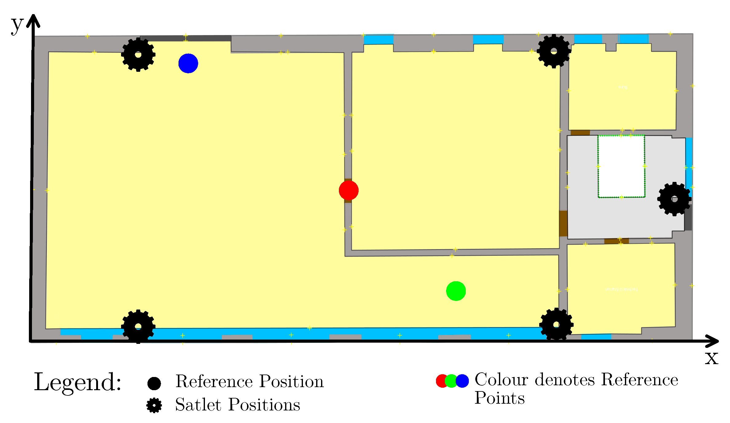
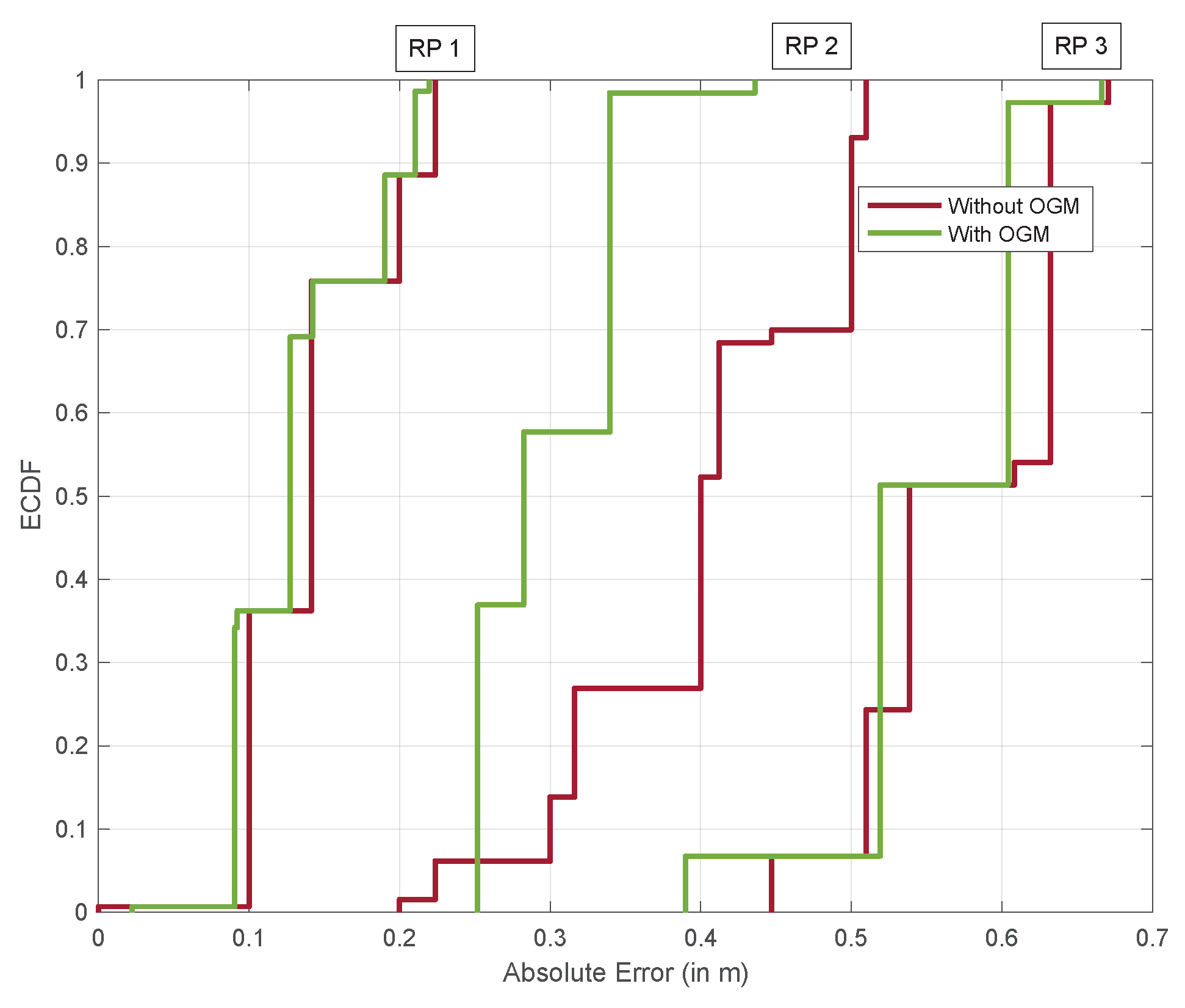
| RP 1 (Red) | RP 2 (Green) | RP 3 (Blue) | |||||||
|---|---|---|---|---|---|---|---|---|---|
| without OGM | 0.06 | 0.12 | 0.14 | 0.04 | 0.40 | 0.40 | 0.86 | 0.71 | 1.12 |
| with OGM | 0.06 | 0.11 | 0.13 | 0.07 | 0.28 | 0.30 | 0.85 | 0.72 | 1.12 |
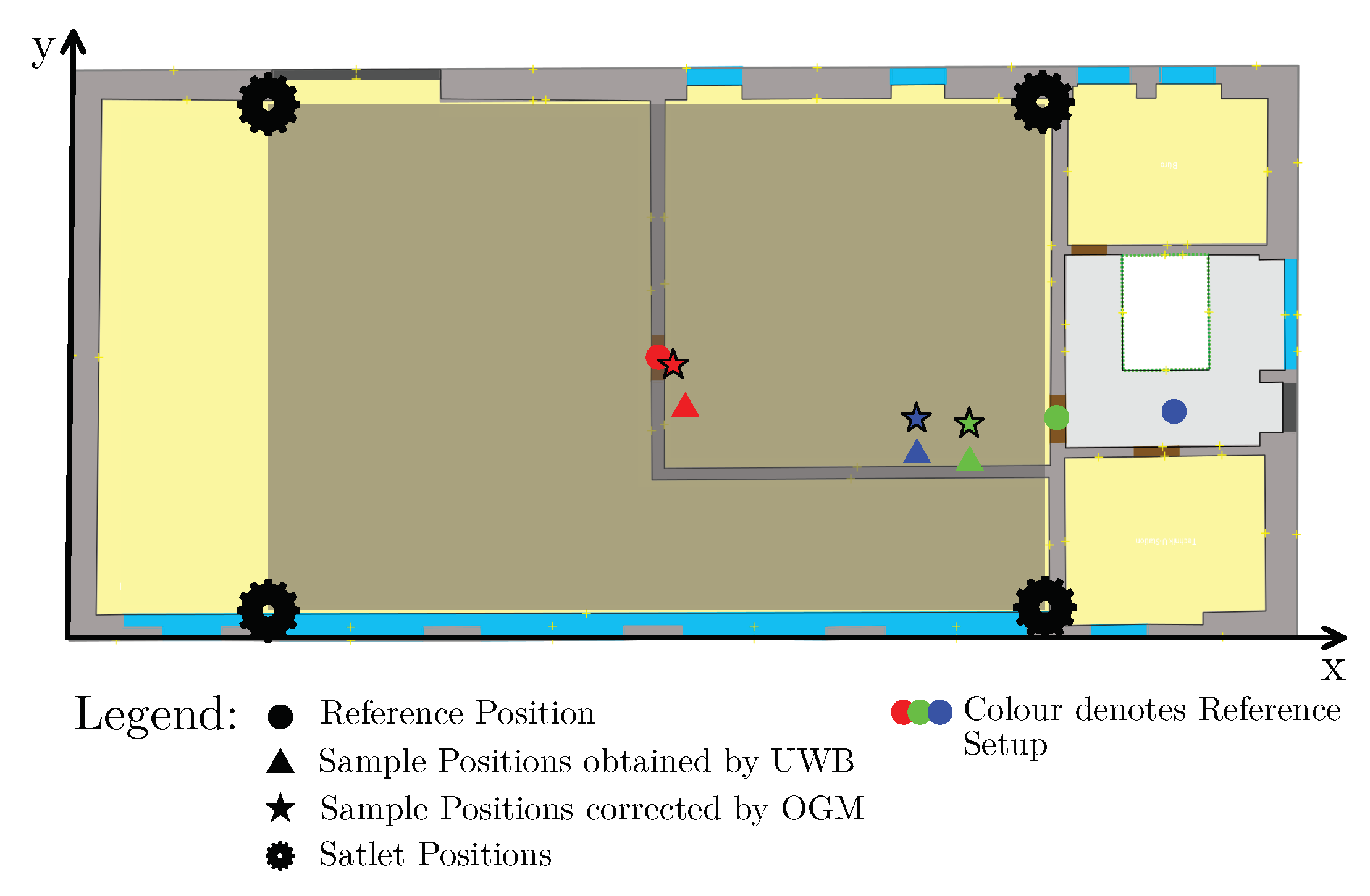
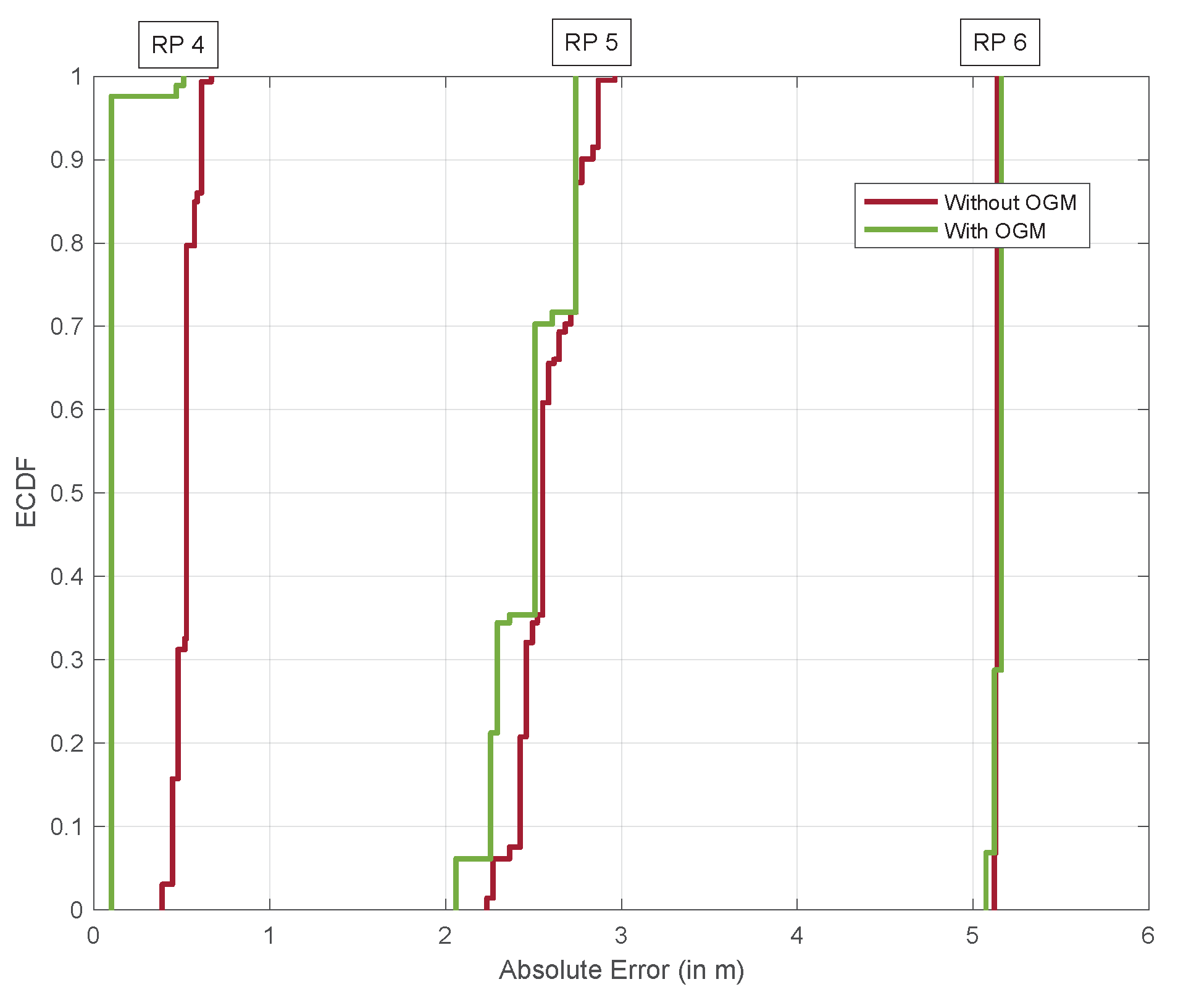
| RP 4 (Red) | RP 5 (Green) | RP 6 (Blue) | |||||||
|---|---|---|---|---|---|---|---|---|---|
| without OGM | 0.27 | 0.44 | 0.52 | 2.44 | 0.84 | 2.58 | 5.11 | 0.50 | 5.13 |
| with OGM | 0.07 | 0.08 | 0.11 | 2.47 | 0.21 | 2.48 | 5.15 | 0.09 | 5.15 |
Publisher’s Note: MDPI stays neutral with regard to jurisdictional claims in published maps and institutional affiliations. |
© 2021 by the authors. Licensee MDPI, Basel, Switzerland. This article is an open access article distributed under the terms and conditions of the Creative Commons Attribution (CC BY) license (https://creativecommons.org/licenses/by/4.0/).
Share and Cite
Graichen, T.; Richter, J.; Schmidt, R.; Heinkel, U. Improved Indoor Positioning by Means of Occupancy Grid Maps Automatically Generated from OSM Indoor Data. ISPRS Int. J. Geo-Inf. 2021, 10, 216. https://doi.org/10.3390/ijgi10040216
Graichen T, Richter J, Schmidt R, Heinkel U. Improved Indoor Positioning by Means of Occupancy Grid Maps Automatically Generated from OSM Indoor Data. ISPRS International Journal of Geo-Information. 2021; 10(4):216. https://doi.org/10.3390/ijgi10040216
Chicago/Turabian StyleGraichen, Thomas, Julia Richter, Rebecca Schmidt, and Ulrich Heinkel. 2021. "Improved Indoor Positioning by Means of Occupancy Grid Maps Automatically Generated from OSM Indoor Data" ISPRS International Journal of Geo-Information 10, no. 4: 216. https://doi.org/10.3390/ijgi10040216