An end-to-end text spotter with text relation networks

Abstract

Reading text in images automatically has become an attractive research topic in computer vision. Specifically, end-to-end spotting of scene text has attracted significant research attention, and relatively ideal accuracy has been achieved on several datasets. However, most of the existing works overlooked the semantic connection between the scene text instances, and had limitations in situations such as occlusion, blurring, and unseen characters, which result in some semantic information lost in the text regions. The relevance between texts generally lies in the scene images. From the perspective of cognitive psychology, humans often combine the nearby easy-to-recognize texts to infer the unidentifiable text. In this paper, we propose a novel graph-based method for intermediate semantic features enhancement, called Text Relation Networks. Specifically, we model the co-occurrence relationship of scene texts as a graph. The nodes in the graph represent the text instances in a scene image, and the corresponding semantic features are defined as representations of the nodes. The relative positions between text instances are measured as the weights of edges in the established graph. Then, a convolution operation is performed on the graph to aggregate semantic information and enhance the intermediate features corresponding to text instances. We evaluate the proposed method through comprehensive experiments on several mainstream benchmarks, and get highly competitive results. For example, on the SCUT-CTW1500, our method surpasses the previous top works by 2.1% on the word spotting task.

Introduction

Automatically spotting text in images has attracted significant research attention in not only academic communities, but also industries, owing to its extensive applications in cybersecurity such as confidentiality checking, public opinion analysis, and computer forensics. Text spotting is customarily the first step to obtain the semantic text in images. In the confidentiality checking and computer forensics tasks, spotted text can be used as a crucial foundation for judging the security of files or computer systems. In public opinion analysis tasks, texts in images are crucial to analyze the themes and emotional trends of community activities, which provide valuable references for maintaining public safety.

Previously, scene text spotting can be further decomposed as text detection and text recognition. Among them, text detection aims to localize text instances (words or text lines) in images. Then text recognition crops text regions from images and then decodes image patches into textual content. The aforementioned procedure is straightforward and simple, but it overlooks the synergy between sub-tasks and can be suffering from sub-optimal. Furthermore, handling detection and recognition separately gives rise to computational redundancy in feature extraction.

Fortunately, end-to-end text spotting models (Liu et al. 2018; Liu et al. 2019a; Feng et al. 2019; Qiao et al. 2020; Lyu et al. 2018) have been available to address the above drawbacks, by handling detection and recognition with an end-to-end trainable neural network. An end-to-end text spotting framework can be roughly divided into three parts: shared feature backbone, detector, and recognizer. The detector and recognizer are jointly trained, hence the whole model can handle both tasks in a single inference step. Nevertheless, the diversity and imperfection of scene texts lead to those spotting remains challenging. On one hand, the diversity of scene texts comes from changes in shape or style, such as varying orientations and curving. In recent years, various works on end-to-end text spotting of arbitrary shaped text (Liu et al. 2019a; Feng et al. 2019; Qiao et al. 2020; Lyu et al. 2018) have achieved relatively ideal accuracy on several established datasets (Ch’ng and Chan 2017; Liu et al. 2019b). On the other hand, most of the existing works did not consider the imperfection of the scene text and had limitations in situations that cause loss of semantic information in scene text regions, such as blurring, occlusion, and unseen characters. Therefore, handling imperfect text remains an open problem in scene text spotting.

Intuitively, The relevance between texts generally lies in the scene images. As shown in Fig. 1, “COFFEE” and “CAFE”, “FITNESS” and “CENTER”, “HARBOR” and “WHARF”, etc., these relevant words appear in the same scene. From the perspective of cognitive psychology, when human beings encounter texts that cannot be recognized, they often combine the nearby easy-to-recognize texts to infer the unidentifiable text. Inspired by the above intuition, our work aims to model the co-occurrence of scene texts, to aggregate semantic information from neighbour regions of text instances, and to enhance the intermediate semantic features of the recognition branch for better recognition performance.

Fig. 1

Examples of real scene text images from Total-Text

In this paper, we propose a novel graph-based method for intermediate semantic features enhancement in end-to-end text spotting, called Text Relation Networks (TRN). We model the co-occurrence relationship of scene texts as a graph. The nodes in the graph represent the text instances in a scene image. The relative spatial positions between text instances and the high-order semantic features corresponding to the text instances are defined as the weights of edges and the representations of nodes in the graph structure, respectively. Then, a convolution operation is performed on the graph to aggregate semantic information and enhance the intermediate semantic features. TRN substantially improves the recognition accuracy on the end-to-end task, without a significant increase in the time complexity. Comprehensive experiments on three mainstream benchmarks show highly competitive results. Specially, on the SCUT-CTW1500, our method surpasses the previous top methods by 2.1% on the word spotting task. In addition, the method can be plugged into most of the existing text spotting framework without any need for additional labeled data. We also apply our method to a concrete security appraisal task, sensitive keywords checking, and evaluate the effectiveness of our method in the text-rich parade scenario and text-poor cover page scenario.

In summary, the main contributions of this paper are as follows:

• We propose a novel graph-based intermediate semantic features enhancement method for scene text spotting, called Text Relation Networks. The method substantially improves the performance on the end-to-end task, while increasing negligible time complexity.

• We plug the TRN into a simple end-to-end text spotting model. The model achieves competitive results on several mainstream benchmarks.

• To the best of our knowledge, this is the first work that handles scene text spotting, by modeling the co-occurrence relationship between text instances and enhancing intermediate semantic features with a graph-based model.

The rest parts of this paper are organized as follows: The related works are reviewed in “Related works” section. For the methodology, We pose an overview of the proposed framework and describe in detail the main components of the proposed method in “Method” section, i.e. text detection branch, text relation networks, and text recognition branch. The experiments are presented and analyzed in “Experiments” section. Finally, the conclusion and the future work are envisaged in “Conclusion” section.

Related works

In recent years, research on scene text has received extensive attention from the research community. In this section, we will briefly review existing work on scene text spotting, graph convolutional neural networks, and visual reasoning.

Scene text spotting

Initially, works such as (Liao et al. 2017) and (Liao et al. 2018) split the text spotting process into two separate stages: text detection and text recognition. They firstly crop text regions from the scene image consulting the results of the detector, then input the patches into the recognizer for recognition.

Recently, in (Liu et al. 2018; Qin et al. 2019; Wang et al. 2020; Lyu et al. 2018; Xing et al. 2019), end-to-end methods which localize and recognize text in a unified model have been proposed. In (Liu et al. 2018), the detector outputs rotated rectangles and then uses a CTC-based recognizer, though it can not handle the curved texts (Shi et al. 2016). Aiming at spotting the arbitrary-shaped text, (Qin et al. 2019; Wang et al. 2020; Lyu et al. 2018; Xing et al. 2019) are proposed. In (Qin et al. 2019), the text instances are detected by the detector based on (He et al. 2017) in mask format, recognized by a Long short-term memory (LSTM) decoder with attention (Luong et al. 2015). In Wang et al. (2020), the detector localizes a set of points on the boundary of each text instance and recognizes texts based on (Shi et al. 2018). (Lyu et al. 2018; Xing et al. 2019) tackle text detection and recognition via instance segmentation, but need extra character-level annotations for training, and hence with a high computational cost. Among them, (Liu et al. 2018; Qin et al. 2019; Wang et al. 2020) follow the same paradigm: text region features are extracted based on results from the detector, and are input into the subsequent recognizer.

The above methods focus on handling the diversity of scene text, such as rotating and curving. However, these works impractically assume the perfection of the scene text and perform poorly in situations with the loss of semantic information, such as blurring and occlusion.

Graph convolutional neural networks

Graph Convolutional Neural Networks (GCNs) are the generalization of convolutional neural networks (CNNs) to graphs. Advances in this direction are generally categorized as spectral and spatial approaches. Specially, Spectral approaches define the convolution operation in the Fourier domain, then perform convolutions in the spectral domain as multiplications in the Euclidean domain (Kipf and Welling 2016; Defferrard et al. 2016). Spatial approaches define the convolutions on the graph, performing patch operation on spatially close neighbours (Bronstein et al. 2017; Monti et al. 2017). For instance, (Monti et al. 2017) proposes a general formulation of spatial approaches MoNet. It uses a mixture of Gaussian as the patch operator. (Veličković et al. 2017) proposes graph attention network (GAT), incorporating the attention mechanism into the signal propagation step.

The aforementioned works represent the nodes in a graph as 1-dimensional vectors, rather than 3-dimensional feature maps. For this reason, the methods cannot directly handle 3-dimensional feature maps, which are used in mainstream computer vision tasks frequently. Moreover, it will lead to extensive cost of the amount of calculation, if we simply flatten 3-dimensional feature maps into 1-dimensional feature vectors.

Visual reasoning

Visual reasoning aims to gather the spatial and semantic information in images, and performs reasoning for the results of specific tasks. Semantic connection between instances is important information for visual reasoning, which is difficult to be represented accurately in Euclidean space, though being natural with a graph. Obviously, GCNs are feasible for extracting features from graphs effectively.

The examples of using GCN in visual reasoning can be found in many computer vision tasks, such as visual question answering (VQA), object detection, and interaction detection. For VAQ, (Teney et al. 2017) proposes to produce a graphical representation of an image conditioned on a question, and performs convolution operation based on MoNet to get the feature for answer classification. For object detection, (Xu et al. 2019) models the proposals in the Faster R-CNN (Ren et al. 2015) as nodes in a graph and enhances the feature for bounding box regression and classification by fusing semantic features of regions of interest (RoIs). For interaction detection, GCN can be used for message passing between humans and objects (Qi et al. 2018). According to the above works, GCNs are excellent aggregators of information on the graph structures which can effectively leverage the semantic and spatial relevance of instances.

Specifically, in Teney et al. (2017); Xu et al. (2019), the detectors are able to perform better bounding box regression and classification, utilizing contexts aggregated from neighbouring proposals. However, the number of proposals is fixed in a two-stage detector, therefore the methods cannot adapt to the dynamic change in the number of nodes.

Method

In this section, we propose the framework of our text spotting model in detail. The framework consists of four parts: shared backbone, text detection branch, text relation networks (TRN), and recognition branch.

Architecture

As illustrated in Fig. 2, the overall architecture of the proposed text spotting model can be described as follows:

• We apply the ResNet-50 (He et al. 2016) with feature pyramid networks (FPN) (Lin et al. 2017) as the shared backbone.

  Fig. 2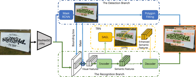

  

  Overall architecture of our spotting model

• The text detection branch is based on Mask R-CNN, which predicts the text bounding boxes and the corresponding text instance segmentation masks.

• The text relation networks (TRN), learn a region-to-region undirected graph for detected text instances, aggregate visual features and semantic features in the recognition branch, and output the enhanced semantic features.

• In the text recognition branch, RoI features from the shared backbone are encoded into semantic features by the encoder, and the decoder decodes the enhanced features from TRN into text sequences.

Text detection branch

In the text detection branch, we follow the standard Mask R-CNN (He et al. 2017) implementation. Firstly, a region proposal network (RPN) is used to predict proposals of text instances. Secondly, the text proposals are then fed into three prediction heads: a classification head to distinguish whether the region is text instance or not, a regression head of bounding boxes to predict coordinates of bounding boxes, and a mask prediction head to predict segmentation masks corresponding to text instance.

Following the recommendation in He et al. (2017), we use hyper-parameters of anchors in the RPN as following: five scales (32,64,128,256,512) corresponding to five stages in FPN (P₂,P₃,P₄,P₅,P₆), and three aspect ratios (0.5,1.0,2.0) in each stage. In the classification head and regression head, 7×7 RoI features are fed in, Aiming at archiving better performance in mask prediction, RoI Align is adopted to extract RoI features, and to preserve more accurate location information. In the mask prediction head, 14×14 RoI features are input, and the output size is 28×28. Non-maximum suppression (NMS) is adopted to remove highly overlapping proposals with an intersection-over-union (IoU) threshold set to 0.7, then 2000 proposals are fed into the following prediction heads. We also adopt NMS to the predicted bounding boxes in the inference stage, the top 1000 boxes are sent to the mask prediction head.

Text relation networks

Aiming at improving the recognition performance of scene text by aggregating information from neighbour text instances and enhancing the corresponding intermediate semantic feature, we propose a graph-based semantic features enhancement method, called Text Relation Networks (TRN).

The co-occurrence relationship of scene texts is modeled as an undirected graph. The undirected graph is formulated as $\mathcal {G=\{N,\varepsilon \}}$, where $\mathcal {N}$ is the set of nodes corresponding to text instances in the image, and $e_{i,j} \in \mathcal {\varepsilon }$ are the edges encoding the co-occurrence relationship between two text instances.

As shown in Fig. 3, the TRN consists of three parts: merge layer (MergeLayer), spatially adaptive graph learner (SAGL), and graph feature pyramid network (GFPN). In order to learn the connections between text instances not only at the visual level but also at the semantic level, the sub-sampled visual features and the semantic features are concatenated and input into a 3×3 convolutional layer called “MergeLayer”. Then the merged features are obtained as the input for the following parts. The SAGL can learn a sparse adjacency matrix from the merged features. In the Graph Feature Pyramid Network (GFPN), the merged features corresponding to the graph produced by the SAGL, are aggregated and fused from their neighbors using a graph CNN approach designed for 3-dimensional feature maps (named “2D-GCN”). And the output features from two 2D-GCN layers are merged in a pyramid style, like (Lin et al. 2017). Subsequently, the output features from GFPN are fed into a decoder of the recognition branch.

Fig. 3

Architecture of text relation networks

Spatially adaptive graph learner

Following the aforementioned formulation of a graph, The adjacency matrix $\mathcal {\varepsilon } \in \mathbb {R}^{n_{t} \times n_{t}}$ needs to be defined, where n_r is the number of text regions produced by the detection branch, then the node neighbourhood can be identified.

At first, the merged features with the size of (n_r,c_m,H,W) are input into a 3×3 convolutional layer and a fully-connected layer, where the output sizes are (n_r,c_e,H,W) and (n_r,D_e), respectively, $c_{e} = \frac {H \times W}{D_{e}}$.

At this point, the merged features are encoded into embedding feature vectors $f_{e} \in \mathbb {R}^{D_{e}}$. Then the visual embedding feature vectors are input into two fully-connected layers of size D_h. And the vectors are concatenated to an embedding feature matrix $F_{e} \in \mathbb {R}^{n_{r} \times D_{h}}$. Thus, the adjacency matrix ε can be defined as following:

$$\begin{array}{@{}rcl@{}} \varepsilon = F_{e}F_{e}^{\mathrm{T}},\ {\varepsilon}_{i,j} = {f_{e}^{i}}^{\mathrm{T}}{f_{e}^{j}}. \end{array} $$

(1)

Nevertheless, not all text instances are highly correlated with the others, and the redundant edges will lead to greater computation cost. Thus, in the SAGL, a sparse neighbourhood system for each node is needed. For each row of the adjacency matrix, we only keep the N_neighbour elements with the highest response value. The process can be formulated as: Neighbour_i=TopN_neighbour(ε_i). SAGL keeps only N_neighbour neighbours with the strongest connection for each node and determines the edges of the graph $\mathcal {G}$.

Graph feature pyramid network

With the sparse undirected graph given by SAGL, the representations of nodes and the patch operations in the graph are defined. In the GFPN, in order to aggregate sufficient efficacious semantic information from neighbouring text regions, firstly, the merged semantic features $F_{m} \in \mathbb {R}^{n_{t} \times c_{m} \times H \times W}$ are subsampled by a 3×3 convolutional layer and a 2×2 max-pooling layer, and the representations $F_{st} \in \mathbb {R}^{n_{t} \times c_{st} \times \frac {H}{2} \times \frac {W}{2}}$ of nodes $\mathcal {N}$ are then obtained.

Inspired by Monti et al. (2017); Teney et al. (2017); Xu et al. (2019), we introduce a graph CNN approach named “2D-GCN”, which performs directly in the graph domain and heavily relies on the spatial relationships. Moreover, we use a pairwise pseudo-coordinate function u(i,j) to capture pairwise spatial relationships. For each node i, u(i,j) will return the corresponding coordinate of node j. u(i,j) is defined as the following polar function: u(i,j)=(d,θ), where d and θ are the distance and the angle of two bounding box centers ([x_i,y_i],[x_j,y_j])

Inspired by Monti et al. (2017), K Gaussian kernels with convolutional layers are applied as the patch operations in the learned graph, which can be formulated as:

$$\begin{array}{@{}rcl@{}} w_{k}(u(i,j))\,=\,\exp\!\left(\!-\frac{1}{2}(u(i,j)\,-\,\mu_{k})^{\mathrm{T}} \Sigma_{k}^{-1}(u(i,j)\,-\,\mu_{k})\!\right),\ \end{array} $$

(2)

$$\begin{array}{@{}rcl@{}} f_{k}^{agg}(i)=\sum_{j \in Neighbour_{i}}w_{k}(u(i,j))f_{s}^{j} {\varepsilon}_{i,j}, \end{array} $$

(3)

$$\begin{array}{@{}rcl@{}} f_{k}(i)=Conv2D(f_{k}^{agg}(i)), \end{array} $$

(4)

where w_k(u(i,j)) is the k-th Gaussian kernel, μ_k and Σ_k are learnable mean and covariance, $f_{k}^{agg}(i)$ is aggregated feature of one kernel, and Conv2D() is a 3×3 convolutional layer of which input and output channel size are c_st and $\frac {c_{st}}{K}$, respectively.

Then we concatenate f_k(i) into $f_{e}^{i} \in \mathbb {R}^{c_{st} \times \frac {H}{2} \times \frac {W}{2}}$ and input the features into a 3×3 convolutional layer to merge the output features from kernels. As shown in Fig. 3, following two 2D-GCN layers, we resize and concatenate the produced features in a pyramid style, as in Lin et al. (2017), so that the GFPN can effectively aggregate and fuse semantic information from neighbours not only in the graph domain but also in the spatial domain.

Text recognition branch

The text recognition branch encodes RoI features and decodes the enhanced features from TRN into text sequences. We use a Gate Recurrent Unit (GRU) model (Cho et al. 2014) with Bahdanau-style attention (Luong et al. 2015) as the decoder. The parameters are shown in Table 1, where “GRU with Attention” stands for attentional GRU decoder, and N_char represents the size of the decoded charset. We set the size of decoded charset in our experiments to 97, which corresponds to digits (0-9), English characters (a-z/A-Z), one category representing all other symbols (Chinese characters and special symbols), and an end-of-sequence symbol. We also adopt the RoI Masking (Qin et al. 2019) to enhanced semantic features, and flatten the features to $F \in \mathbb {R}^{n_{t} \times (H \times W) \times 256}$. Then the attention model translates F into a text symbol sequence y=(y₁,…,y_T), where T is the length of the label sequence. At the t step, the prediction distribution over possible labels is formulated as the following:

$$\begin{array}{@{}rcl@{}} p(y_{t}|y_{1},\ldots,y_{t-1},F)=Softmax(W_{o}g_{t}+b_{o}), \end{array} $$

(5)

Table 1 The architecture of the recognition branch

where Wo and b_o are learnable parameters, and g_t is GRU output at time step t. At each time step, GRU takes the output y_t−1, hidden state s_t−1 of previous time step t−1 and context c_t. One time step of GRU is calculated according to the following: (g_t,s_t)=GRU(y_t−1,s_t−1,c_t). c_t is a weighted sum of the flattened features F, allowing the decoder focusing on features critical at the current time step. c_t is calculated according to following:

$$\begin{array}{@{}rcl@{}} c_{t}=\sum_{i=1}^{n}\alpha_{t,i}F_{i}, \end{array} $$

(6)

$$\begin{array}{@{}rcl@{}} \alpha_{t,i}=\frac{\exp(e_{t,i})}{\sum_{j=1}^{j}\exp(e_{t,j})}, \end{array} $$

(7)

$$\begin{array}{@{}rcl@{}} e_{t,i}=W_{a}^{\mathrm{T}}tanh(W_{s}s_{t-1}+VF_{i}+b), \end{array} $$

(8)

where W_a,W_s, V, and b are learnable parameters.

The loss function of the text recognition branch can be formulated as:

$$\begin{array}{@{}rcl@{}} L_{recog}=-\frac{1}{T}\sum_{t=1}^{t}\log p(y_{t}|y_{1},\ldots,y_{t-1},F). \end{array} $$

(9)

Combined with detection loss, the full multi-task loss function is formulated as:

$$\begin{array}{@{}rcl@{}} L=L_{detect}+\lambda L_{recog}, \end{array} $$

(10)

$$\begin{array}{@{}rcl@{}} L_{detect}=L_{rpn}+\alpha L_{rcnn}+\beta L_{mask}, \end{array} $$

(11)

where the detection loss L_detect is the same as the original Mask R-CNN paper (He et al. 2017). Hyper-parameter λ,α, and β control the trade-off between the losses. In addition, λ,α, and β are set to 1 in our experiments.

Experiments

In order to evaluate the effectiveness of our proposed method on arbitrary-shaped text spotting, we conduct extensive experiments on three popular scene text benchmark datasets: a straight text dataset ICDAR 2015, and two curved text datasets Total text and SCUT-CTW1500. In this section, first, the datasets used for training and testing, and the experiment settings are described. Next, our method is evaluated on the three benchmarks and compared with other state-of-the-art methods. Then, we further analyze the performance of our method by performing ablation studies and visualization. Finally, The proposed method is applied to sensitive keywords checking of images, and evaluated in multiple scenarios.

Datasets

SynthText

SynthText dataset (Gupta et al. 2016) is a synthetic dataset with around 800000 images. The texts in this dataset are multi-oriented. And the text instances are annotated with rotated bounding boxes in word-level and character-level, as well as transcriptions.

ICDAR 2015

ICDAR 2015 dataset (Karatzas et al. 2015) focuses on detection and recognition of multi-oriented scene text in natural images. There are 1000 images for training and 500 for testing in the dataset, which are annotated with quadrangles and corresponding transcriptions only at word-level.

Total-Text

Total-Text dataset (Ch’ng and Chan 2017) is a crucial arbitrarily-shaped scene text benchmark, which contains horizontal, multi-oriented, and curved text in the images. There are 1255 training images and 300 test images in the Total-Text. The images are annotated with polygons and corresponding transcriptions at the word level. Most of the images in the Total-Text contain a large amount of regular text (horizontal text or multi-oriented text) and at least one curved text.

SCUT-CTW1500

SCUT-CTW1500 dataset (Liu et al. 2019b) is a challenging dataset for detection and recognition of curved text which consisting of 1000 training images and 500 test images. The text instances in SCUT-CTW1500 are labeled by polygons with 14 vertices and corresponding transcriptions. The dataset contains both Latin and non-Latin (such as Chinese characters) characters. Moreover, the images are annotated at text-line level, and also include some document-like text, so that several small texts may be stacked together and hard to be detected accurately.

Aiming at selecting a suitable dataset to learn relevance between scene texts, we counted the distribution of the number of text instances contained in ICDAR 2015, Total-Text, and SCUT-CTW1500, ignoring the “DO NOT CARE” text instances. Compared to Total-Text and SCUT-CTW1500, as shown in Fig. 4, there are a large number of images with few valid text instances in ICDAR 2015. Therefore, it is more appropriate to explore the semantic connection between text instances on Total-Text and SCUT-CTW1500.

Fig. 4

The numbers of text instances contained in the images in the three datasets

Experiment settings

The shared backbone is pre-trained on the ImageNet dataset (Deng et al. 2009). We adopt a multi-step strategy to the training stage, which includes two steps: firstly, the model is pre-trained on SynthText dataset, then, scene images from the real world are adopted to fine-tune the network.

During the training phase, the batch size is set to 3 for all experiments. In the text detection branch, the batch size of RPN, Fast R-CNN (classification head and regression head share the same input features) and mask prediction are 512, 256, and 64, respectively. To train the detection branch, TRN, and the recognition branch jointly, the batch sizes of the three modules are set to be equivalent. In the SAGL, we set the dimension of embedding vectors D_e to 1024, following linear layers in size of 512 and N=4 neighbours of each node are retained. In the GFPN, we set hidden state channels of nodes c_st to 128, and we use two graph convolution layers with the same hidden state channels for reasoning in the graph. In the pre-training stage, the shorter side of all input images is resized to 800, keeping the aspect ratio. In the fine-tuning stage, data augmentation is applied. First, shorter sides of images are resized to three sizes (600,800,1000) randomly. Next, we adopt random cropping, making sure that no text is cut. The training images are collected from ICDAR 2013, ICDAR 2015, Total-Text, and SCUT-CTW1500.

Our model is optimized with the SGD with weight decay of 0.0001 and momentum of 0.9. During pre-training, we train our model for 600k iterations, with an initial learning rate of 0.004, and decay learning rate to 0.0004 and 0.00004 at the 200k and 400k iteration, respectively. In the fine-tuning stage, the initial learning rate is set to 0.0004 and then is decreased to a tenth at the 100k and 200k iteration. The fine-tuning process is finished at the 300k iteration. We implement our method using Pytorch and run all experiments with 3 NVIDIA 2080 Ti GPUs. The model is trained parallel and evaluated on a single GPU, and the training process takes about 6 days to finish.

Experimental results on straight text

To validate the superior performance of our method on the oriented straight scene text, we conduct experiments on ICDAR 2015. During the testing phase, we scale the shorter sides of the images to 1000. In the detection task, a predicted bounding box is taken as a true positive only if the IoU with the closest ground-truth is larger than 0.5. In the end-to-end task, the prediction is considered as a true positive only if the detection matched and predicted transcription is identical to the corresponding ground-truth. For a fair comparison, images of MLT2017 are not used for training, following settings in Lyu et al. (2018). As shown in Table 2, the proposed models get competitive performance. “S”, “W”, and “G” stands for recognition with strong, weak, and generic lexicon respectively. Practically, on the ICDAR 2015 benchmark, our method outperforms previous methods in terms of the detection precision and F-measure of end-to-end recognition with general lexicon by 3.6% and 4.5%, respectively.

Table 2 Results on ICDAR 2015

Experimental results on curved text

Our proposed method focuses on arbitrary-shaped scene text, so we evaluate the proposed method on two curved scene text benchmarks: Total-Text and SCUT-CTW1500. During the testing phase, we scale the shorter sides of the images to 1000, and assess the performance of our model in three tasks: detection, end-to-end recognition, and word spotting.

The performance on Total-Text is given in Table 3. “None” means recognition without any lexicon, and “Full” lexicon contains all words in the test set. Our method achieves comparable performance on both detection and end-to-end recognition. Specifically, our method surpasses the previous works (Lyu et al. 2018; Feng et al. 2019) by 3.8% and 13.2% in the precision of detection and F-measure of end-to-end recognition with none lexicon respectively. For the SCUT-CTW1500 dataset, the performance is reported in Table 4. Our model achieves state-of-the-art performance on the word spotting task.

Table 3 Results on Total-Text

Table 4 Results on CTW1500. * represents the results are from official end-to-end leaderboard

Concluded from the results, the improvement over other methods gives credit to the following points: 1) Compared with previous works, benefiting from enhancing intermediate semantic features of the recognition branch with TRN, our model is able to capture the semantic correlation between text instance and its neighbours, and aggregate semantic features from related neighbours, then achieve better performance. 2) Compared with segmentation based methods (Lyu et al. 2018), the attention-based decoder in our recognition branch can capture the relationship between characters of a text instance and global semantic information, which can significantly promote performance on the recognition task. However, the segmentation based methods predict the characters separately, ignoring the relationship between them. 3) The performance on the detection task can be improved implicitly, due to better performance in the recognition branch and shared backbone.

Ablation study

To confirm the effectiveness of our end-to-end framework and TRN, we conduct several ablation experiments. Based on the analysis of datasets in “Datasets” section, we perform the experiments with the Total-Text test set in this section, which is one of the most important arbitrarily-shaped dataset, and has moderate difficulty in above mentioned three real-world datasets. The results are shown in Tables 3, 5, and 6, and the details are discussed as follows.

Table 5 Ablation study for time consumption and space consumption of TRN

Table 6 Ablation study for size of neighborhoods on Total-Text

Ablation study on the end-to-end manner

To confirm the influence of the recognition branch on the detection task, we build a detection baseline model named “det-baseline”. In the “det-baseline”, we remove the recognition branch and the TRN from our original model, and train the model only on the detection task. As shown in Table 3, our text spotting model outperforms the “det-baseline” by 1.0% F-measure and 2.3% precision on text detection. The result shows that, in virtue of jointly optimizing and shared backbone, the end-to-end manner is able to improve performance on the detection task.

Ablation study on the TRN

To evaluate the effectiveness of the proposed TRN, we train an end-to-end baseline model named “e2e-baseline”. In the “e2e-baseline”, we remove the TRN module from our text spotting model, and train the model with the same setting. Qualitative examples are shown in Fig. 5, where the results from “e2e-baseline” are placed at the top, and the results from the model with TRN are put at the bottom. Moreover, we also consider the runtime per image and the size of the parameters of our models. The results in Tables 2, 3 and 5 show that TRN is able to significantly improve the end-to-end results, while exerting only 5.6% time complexity and 4.5M space consumption. We conduct experiments to confirm the hyper-parameter setting, as shown in Table 6, the size of neighbourhood N_neighbour=4 is the optimal setting on the Total-Text, “F-measure” means F-measure scores of end-to-end recognition with full lexicon on Total-Text with different size of neighbourhood. Practically, we share the same setting on the other datasets.

Fig. 5

Qualitative recognition results of the “e2e-baseline” and our text spotting model

Visualization

In order to evaluate the effectiveness of our method intuitively, in this section, we visualize the results from our method on the above-mentioned benchmarks: ICDAR 2015, Total-Text, and SCUT-CTW1500. The results from the visualization are illustrated in Figs. 6 and 7.

Fig. 6

Examples of text spotting results of our text spotting model on the three datasets

Fig. 7

Visualization of results from our text spotting model with edges learned by TRN

In Fig. 7, the red rectangles and green polygons are predicted bounding boxes and masks from the detection branch respectively. The centers of bounding boxes are plotted and connected by the learned graph edges from the SAGL in the TRN. The thickness of lines stands for the strength of the graph edge weights. For the conciseness of figures, we choose one detected text instance from each image randomly, and only visualize graph edges corresponding to the neighbourhoods of the text instance.

As shown in Figs. 6 and 7, our method can accurately detect and recognize most of the arbitrarily-shaped scene text in the aforementioned real-world datasets. In virtue of the TRN, our method could discover semantic connections between text instances and fuse semantic information from neighbours, then achieve better performance on several complicated text instances. For example, in Fig. 7, in the bottom right figure, text instances with similar appearance characteristics (e.g. font, color) or the same textual content are connected. Their intermediate semantic features thus are shared and enhanced. Furthermore, in the other two figures, text instances with semantic connection or co-occurrence are connected e.g. “HARBOR” and “FISHING”; “HARBOR” and “WHARF”; “CRAWFISH” and “SEAFOOD’ ’ and “CRAWFISH” and “CRAB”. The correct learned edges help the successful graph reasoning thus lead to better spotting performance.

Practical applications

In this subsection, we apply our method to a concrete security appraisal task, sensitive keywords checking, which is a critical step for public opinion analysis and file confidentiality checking. Our method is evaluated in two different scenarios, text-rich parade scenario and text-poor cover page scenario.

We collect a series of representative images from the two scenarios from Internet, and perform the keywords checking task. Firstly, the text instances in images are spotted with our model which trained at the proposed experiment settings. Afterwards, the spotted texts are then compared with each keyword, and the text with a string similarity higher than 0.65 with keywords will be hit, otherwise it will be passed.

As shown in Fig. 8, in the top two figures which are from the text-rich parade scenario, our method can spot most of the text instances in images, and hit the keywords with our string similarity based matching strategy. In the bottom two figures of text-poor cover page, the text instances are spotted accurately, and the corresponding keywords are hit subsequently. Our method is effective on keywords checking, and shows sufficient robustness to different scenarios, text-rich parade scenario and text-poor cover page scenario. In practical applications, our method can prevent the revelation of sensitive or confidential information, and contribute to maintaining content security in cyberspace.

Fig. 8

Keywords checking results from our method in the parade scenario and cover page scenario

Conclusion

Humans generally combine the nearby easy-to-read texts to infer the unidentifiable text. In other words, the semantic relevance between scene texts contains vital information for reading of imperfect texts, and hence, the utilization of semantic relevance between text instances is essential for more accurate text spotting.

In this work, we propose a novel graph-based intermediate semantic features enhancement method for scene text spotting, called Text Relation Networks (TRN). In the TRN, the co-occurrence relationship of scene texts is modeled as a sparse undirected graph. Subsequently, the intermediate features corresponding to text instances are enhanced by performing convolution operation on the constructed graph. TRN is able to easily plugged into existing end-to-end text spotting frameworks. Our simple text spotting model with TRN achieves highly competitive results on the end-to-end task, compared with popular methods with more compact structures. In the future, we would like to explore the relevance between text instances at a deeper semantic level, and the detection branch can also be predigested in a single-stage style.

References

Bronstein, MM, Bruna J, LeCun Y, Szlam A, Vandergheynst P (2017) Geometric deep learning: going beyond euclidean data. IEEE Signal Process Mag 34(4):18–42.
Ch’ng, CK, Chan CS (2017) Total-text: A comprehensive dataset for scene text detection and recognition In: 2017 14th IAPR International Conference on Document Analysis and Recognition (ICDAR), vol. 1, 935–942.. IEEE, Los Alamitos.
Cho, K, Van Merrienboer B, Gulcehre C, Bahdanau D, Bougares F, Schwenk H, Bengio Y (2014) Learning phrase representations using rnn encoder-decoder for statistical machine translation. Comput ence abs/1406.107. http://arxiv.org/abs/1406.1078.
Defferrard, M, Bresson X, Vandergheynst P (2016) Convolutional neural networks on graphs with fast localized spectral filtering In: Advances in Neural Information Processing Systems, 3844–3852.. Curran Associates Inc., Red Hook.
Deng, J, Dong W, Socher R, Li L-J, Li K, Fei-Fei L (2009) Imagenet: A large-scale hierarchical image database In: 2009 IEEE Conference on Computer Vision and Pattern Recognition, 248–255.. IEEE Computer Society, Los Alamitos.
Feng, W, He W, Yin F, Zhang X-Y, Liu C-L (2019) Textdragon: An end-to-end framework for arbitrary shaped text spotting In: Proceedings of the IEEE International Conference on Computer Vision, 9076–9085.. IEEE Computer Society, Los Alamitos.
Gupta, A, Vedaldi A, Zisserman A (2016) Synthetic data for text localisation in natural images In: Proceedings of the IEEE Conference on Computer Vision and Pattern Recognition, 2315–2324.
He, K, Gkioxari G, Dollár P, Girshick R (2017) Mask r-cnn In: Proceedings of the IEEE International Conference on Computer Vision, 2961–2969.. IEEE Computer Society, Los Alamitos.
He, T, Tian Z, Huang W, Shen C, Qiao Y, Sun C (2018) An end-to-end textspotter with explicit alignment and attention In: Proceedings of the IEEE Conference on Computer Vision and Pattern Recognition, 5020–5029.. IEEE Computer Society, Los Alamitos.
He, K, Zhang X, Ren S, Sun J (2016) Deep residual learning for image recognition In: Proceedings of the IEEE Conference on Computer Vision and Pattern Recognition, 770–778.. IEEE Computer Society, Los Alamitos.
Karatzas, D, Gomez-Bigorda L, Nicolaou A, Ghosh S, Bagdanov A, Iwamura M, Matas J, Neumann L, Chandrasekhar VR, Lu S, et al (2015) Icdar 2015 competition on robust reading In: 2015 13th International Conference on Document Analysis and Recognition (ICDAR), 1156–1160.. IEEE, Los Alamitos.
Kipf, TN, Welling M (2016) Semi-supervised classification with graph convolutional networks. arXiv preprint arXiv:1609.02907.
Liao, M, Shi B, Bai X (2018) Textboxes++: A single-shot oriented scene text detector. IEEE Trans Image Process 27(8):3676–3690.
Liao, M, Shi B, Bai X, Wang X, Liu W (2017) Textboxes: A fast text detector with a single deep neural network In: Thirty-First AAAI Conference on Artificial Intelligence.. IEEE, New York City.
Lin, T-Y, Dollár P, Girshick R, He K, Hariharan B, Belongie S (2017) Feature pyramid networks for object detection In: Proceedings of the IEEE Conference on Computer Vision and Pattern Recognition, 2117–2125.. IEEE Computer Society, Los Alamitos.
Liu, Y, Jin L, Zhang S, Luo C, Zhang S (2019) Curved scene text detection via transverse and longitudinal sequence connection. Pattern Recognit 90:337–345. https://doi.org/10.1016/j.patcog.2019.02.002.
Liu, Y, Jin L, Zhang S, Luo C, Zhang S (2019) Curved scene text detection via transverse and longitudinal sequence connection. Pattern Recog 90:337–345.
Liu, X, Liang D, Yan S, Chen D, Qiao Y, Yan J (2018) Fots: Fast oriented text spotting with a unified network In: Proceedings of the IEEE Conference on Computer Vision and Pattern Recognition, 5676–5685.. IEEE Computer Society, Los Alamitos.
Luong, T, Pham H, Manning CD (2015) Effective Approaches to Attention-based Neural Machine Translation. In: Màrquez L, Callison-Burch C, Su J, Pighin D, Marton Y (eds)Proceedings of the 2015 Conference on Empirical Methods in Natural Language Processing, EMNLP 2015, Lisbon, Portugal, September 17-21, 2015, 1412–1421.. The Association for Computational Linguistics. https://doi.org/10.18653/v1/d15-1166.
Lyu, P, Liao M, Yao C, Wu W, Bai X (2018) Mask textspotter: An end-to-end trainable neural network for spotting text with arbitrary shapes In: Proceedings of the European Conference on Computer Vision (ECCV), 67–83.
Monti, F, Boscaini D, Masci J, Rodola E, Svoboda J, Bronstein MM (2017) Geometric deep learning on graphs and manifolds using mixture model cnns In: Proceedings of the IEEE Conference on Computer Vision and Pattern Recognition, 5115–5124.. IEEE Computer Society, Los Alamitos.
Qi, S, Wang W, Jia B, Shen J, Zhu S-C (2018) Learning human-object interactions by graph parsing neural networks In: Proceedings of the European Conference on Computer Vision (ECCV), 401–417.. Springer, Cham.
Qiao, L, Tang S, Cheng Z, Xu Y, Wu F (2020) Text perceptron: Towards end-to-end arbitrary-shaped text spotting. Proc AAAI Conf Artif Intell 34(7):11899–11907.
Qin, S, Bissacco A, Raptis M, Fujii Y, Xiao Y (2019) Towards unconstrained end-to-end text spotting In: Proceedings of the IEEE International Conference on Computer Vision, 4704–4714.. IEEE Computer Society, Los Alamitos.
Ren, S, He K, Girshick R, Sun J (2015) Faster r-cnn: Towards real-time object detection with region proposal networks In: Advances in Neural Information Processing Systems, 91–99.. Curran Associates Inc., Red Hook.
Shi, B, Bai X, Yao C (2016) An end-to-end trainable neural network for image-based sequence recognition and its application to scene text recognition. IEEE Trans Pattern Anal Mach Intell 39(11):2298–2304.
Shi, B, Yang M, Wang X, Lyu P, Yao C, Bai X (2018) Aster: An attentional scene text recognizer with flexible rectification. IEEE Trans Pattern Anal Mach Intell 41(9):2035–2048.
Sun, Y, Zhang C, Huang Z, Liu J, Han J, Ding E (2018) Textnet: Irregular text reading from images with an end-to-end trainable network In: Asian Conference on Computer Vision, 83–99.. Springer, Cham.
Teney, D, Liu L, van Den Hengel A (2017) Graph-structured representations for visual question answering In: Proceedings of the IEEE Conference on Computer Vision and Pattern Recognition, 1–9.. IEEE Computer Society, Los Alamitos.
Veličković, P, Cucurull G, Casanova A, Romero A, Lio P, Bengio Y (2017) Graph attention networks. arXiv preprint arXiv:1710.10903.
Wang, H, Lu P, Zhang H, Yang M, Liu W (2020) All you need is boundary: Toward arbitrary-shaped text spotting. Proc AAAI Conf Artif Intell 34(7):12160–12167.
Xing, L, Tian Z, Huang W, Scott MR (2019) Convolutional character networks In: Proceedings of the IEEE International Conference on Computer Vision, 9126–9136.. IEEE Computer Society, Los Alamitos.
Xu, H, Jiang C, Liang X, Li Z (2019) Spatial-aware graph relation network for large-scale object detection In: Proceedings of the IEEE Conference on Computer Vision and Pattern Recognition, 9298–9307.. IEEE Computer Society, Los Alamitos.
Zhou, X, Yao C, Wen H, Wang Y, Zhou S, He W, Liang J (2017) East: an efficient and accurate scene text detector In: Proceedings of the IEEE Conference on Computer Vision and Pattern Recognition, 5551–5560.. IEEE Computer Society, Los Alamitos.
Acknowledgements
This work is supported by National Natural Science Foundation of China (No. 61572469).
Funding
Not applicable.
Author information
Authors and Affiliations
Contributions
The author(s) read and approved the final manuscript.
Corresponding author
Ethics declarations
Competing interests
The authors declare that they have no competing interests.
Additional information
Publisher’s Note
Springer Nature remains neutral with regard to jurisdictional claims in published maps and institutional affiliations.
Rights and permissions
Open Access This article is licensed under a Creative Commons Attribution 4.0 International License, which permits use, sharing, adaptation, distribution and reproduction in any medium or format, as long as you give appropriate credit to the original author(s) and the source, provide a link to the Creative Commons licence, and indicate if changes were made. The images or other third party material in this article are included in the article’s Creative Commons licence, unless indicated otherwise in a credit line to the material. If material is not included in the article’s Creative Commons licence and your intended use is not permitted by statutory regulation or exceeds the permitted use, you will need to obtain permission directly from the copyright holder. To view a copy of this licence, visit http://creativecommons.org/licenses/by/4.0/.
About this article
Cite this article
Jiang, J., Wei, B., Yu, M. et al. An end-to-end text spotter with text relation networks. Cybersecur 4, 7 (2021). https://doi.org/10.1186/s42400-021-00073-x
Received:
Accepted:
Published:
DOI: https://doi.org/10.1186/s42400-021-00073-x