Construction of a Landscape Ecological Network for a Large-Scale Energy and Chemical Industrial Base: A Case Study of Ningdong, China

Abstract

A large-scale energy and chemical industry base is an important step in the promotion of the integrated and coordinated development of coal and its downstream coal-based industry. A number of large-scale energy and chemical industrial bases have been built in the Yellow River Basin that rely on its rich coal resources. However, the ecological environment is fragile in this region. Once the eco-environment is destroyed, the wildlife would lose its habitat. Therefore, this area has attracted wide attention regarding the development of the coal-based industry while also protecting the ecological environment. An ecological network could improve landscape connectivity and provide ideas for ecological restoration. This study took the Ningdong Energy and Chemical Industrial Base as a case study. Morphological spatial pattern analysis was applied to extract core patches. The connectivity of the core patches was evaluated, and then the ecological source patches were recognized. The minimum cumulative resistance model, hydrologic analysis and circuit theory were used to simulate the ecological network. Then, ecological corridors and ecological nodes were classified. The results were as follows: (1) The vegetation fractional coverage has recently been significantly improved. The area of core patches was 22,433.30 ha. In addition, 18 patches were extracted as source patches, with a total area of 9455.88 ha; (2) Fifty-eight potential ecological corridors were simulated. In addition, it was difficult to form a natural ecological corridor because of the area’s great resistance. Moreover, the connectivity was poor between the east and west; (3) A total of 52 potential ecological nodes were simulated and classified. The high-importance nodes were concentrated in the western grassland and Gobi Desert. This analysis indicated that restoration would be conducive to the ecological landscape in this area. Furthermore, five nodes with high importance but low vegetation fractional coverage should be given priority in later construction. In summary, optimizing the ecological network to achieve ecological restoration was suggested in the study area. The severe eco-environmental challenges urgently need more appropriate policy guidance in the large energy and chemical bases. Thus, the ecological restoration and ecological network construction should be combined, the effectiveness of ecological restoration could be effectively achieved, and the cost could also be reduced.

1. Introduction

The mining of coal resources could bring huge economic benefits [1]. However, high-intensity industrial coal development would also occupy a large area of habitat patches [2,3], and inevitably aggravate vegetation degradation, desertification, and landscape fragmentation [4,5]. Meanwhile, landscape fragmentation could also reduce the landscape connectivity, and then damage ecosystem health [6,7], thus interfering with the normal landscape ecological process and ecological regulation ability [7]. It would inevitably affect the ecological barrier and restrict sustainable development. During the past decade, there has been an increasing interest in landscape pattern changes in coal mine areas [4,8], and the need for ecological restoration in coal mine areas has elicited widespread concern from scholars [9,10,11].

Currently, China’s Central Government has incorporated the ecological protection and high-quality development of the Yellow River Basin into the major national strategy [12]. The Yellow River Basin is both an important ecological barrier and an energy base in China [13]. The coal production reaches to 2.77 × 10⁹ t·a⁻¹, accounting for 78% of China’s total [14]. Notably, the Aeolian Sand Area is located in the middle reaches of the Yellow River basin. Owing to shallow and abundant coal reserves, this area has attracted two large energy bases, namely, Ningdong and Shendong. However, the eco-environment is extremely fragile and restrained by its drought climate [15]. Moreover, mining operations might induce surface subsidence, and solid wastes such as coal-gangue and coal-cinder may cause soil pollution [9]. Statistically, approximately 0.22 ha of land will be destroyed with per ten thousand tons of coal production in opencast mining areas. Furthermore, solid waste production is as high as 9.3 × 10¹⁰ t·a⁻¹, but the recycling rate is less than 35%. Thus far, the Yellow River Basin has not been well protected, mainly due to the unreasonable coal mining and untimely ecological restoration.

Theoretically, ecological restoration could be workable in any region regardless of cost. However, the reality is that cost must be taken into account [8]. Thus, ecological restoration should be implemented in key areas, which could optimize ecological security patterns. Ecological networks represent an important element for resolving issues related to species and habitat protection [16]. An excellent ecological network structure is the basis of sustainable development for the ecological environment [17], connecting fragmented patches, as well as enhancing ecological connectivity [18,19]. In addition, ecological connectivity depends on landscape structure [20]. A previous study has shown that high landscape connectivity can enhance an ecosystem’s stability [21,22]. Therefore, connectivity is of great significance to ecological security patterns.

The ecological network is composed of ecological source patches, ecological corridors, and ecological nodes [23]. The recognition of source patches is the key to the ecological network, which directly determines the science of the later construction of the ecological network. Generally, source patches constitute natural and semi-natural vegetation, which provides a habitat for local species [24]. However, previous studies directly selected natural vegetation with high habitat quality as source patches [25,26], or selected the source patches according to the ecological index system such as ecosystem service value [27]. They ignored the connectivity of patches in the landscape and had strong subjectivity.

The construction of ecological corridors and ecological nodes is an important part of landscape ecological planning [28]. Ecological corridors can accomplish material flow to protect biodiversity [24]. Meanwhile, ecological nodes can connect adjacent source patches to improve connectivity. Numerous studies show that the minimum cumulative resistance (MCR) model could identify the minimum-cost path and the critical nodes [26,29], so it has been widely applied for investigation in landscape ecology. Furthermore, the circuit theory of physics was introduced into landscape ecology, enabling the simulation of the migration process of species to recognize alternative paths [30]. Additionally, circuit theory can identify ecological nodes based on an electric current model [31]. However, these methods cannot identify the relative importance of corridors and nodes. Therefore, the relative importance of corridors and nodes remains to be quantitatively analyzed, so as to scientifically determine the priority protection order of ecological corridors and ecological nodes. The common methods are the gravity model [24], graph theory [32], relative ecological importance [2,33], assignment weighting [28,34], etc. It should be noted that the corridors generated by MCR are potential corridors, but the existing structural corridors in the landscape are not considered.

Recently, morphological spatial pattern analysis (MSPA) was introduced into ecological network analysis [35]. In contrast to the traditional method, MSPA emphasized structural connection [36], which could distinguish the type and structure of the landscape more accurately by the principle of morphology [37]. The natural and semi-natural vegetation (forest, shrub, grassland, etc.) was extracted as foreground data, and other areas as background data (matrix). Then, the foreground data could be divided into seven types (core; bridge; edge; perforation; islet; loop; and branch) [38], according to their shape by a series of image processing. Thus, MSPA could identify landscape types that are important for maintaining connectivity, which increases the scientific recognition of source patches and ecological corridors.

The major contributions of the present paper pertain to methodological development for analyzing ecological networks. A method to recognize the ecological source patch was proposed by our previous research [2,39,40]. That is, the core patches of the MSPA were analyzed by combining habitat quality, ecosystem service value, and the importance of patch connectivity. Then, the core patches with three indicators all in the top 30 were extracted as the source patches. This study was a further extension to construct an ecological network in a large-scale energy and chemical base on this basis. This investigation considered the Ningdong Energy and Chemical Industrial Base (NECIB, for short) as a case study. Then, the landscape ecological network approach was introduced into ecological restoration. The purposes of this study were as follows: (1) Extract core patches by MSPA, and identify ecological source patches by landscape connectivity indicators; (2) Simulate the potential ecological corridors and the potential ecological nodes, combining the MCR model, circuit theory and hydrological analysis; (3) Analyze the importance of the ecological network, combining the gravity model, circuit theory, and hydrological analysis; (4) Propose the optimization countermeasures for the ecological network to achieve ecological restoration. The results could provide suggestions for the protection and planning of the ecological network for the construction of energy bases in arid and semi-arid regions of the world.

2. Materials and Methods

2.1. Study Area

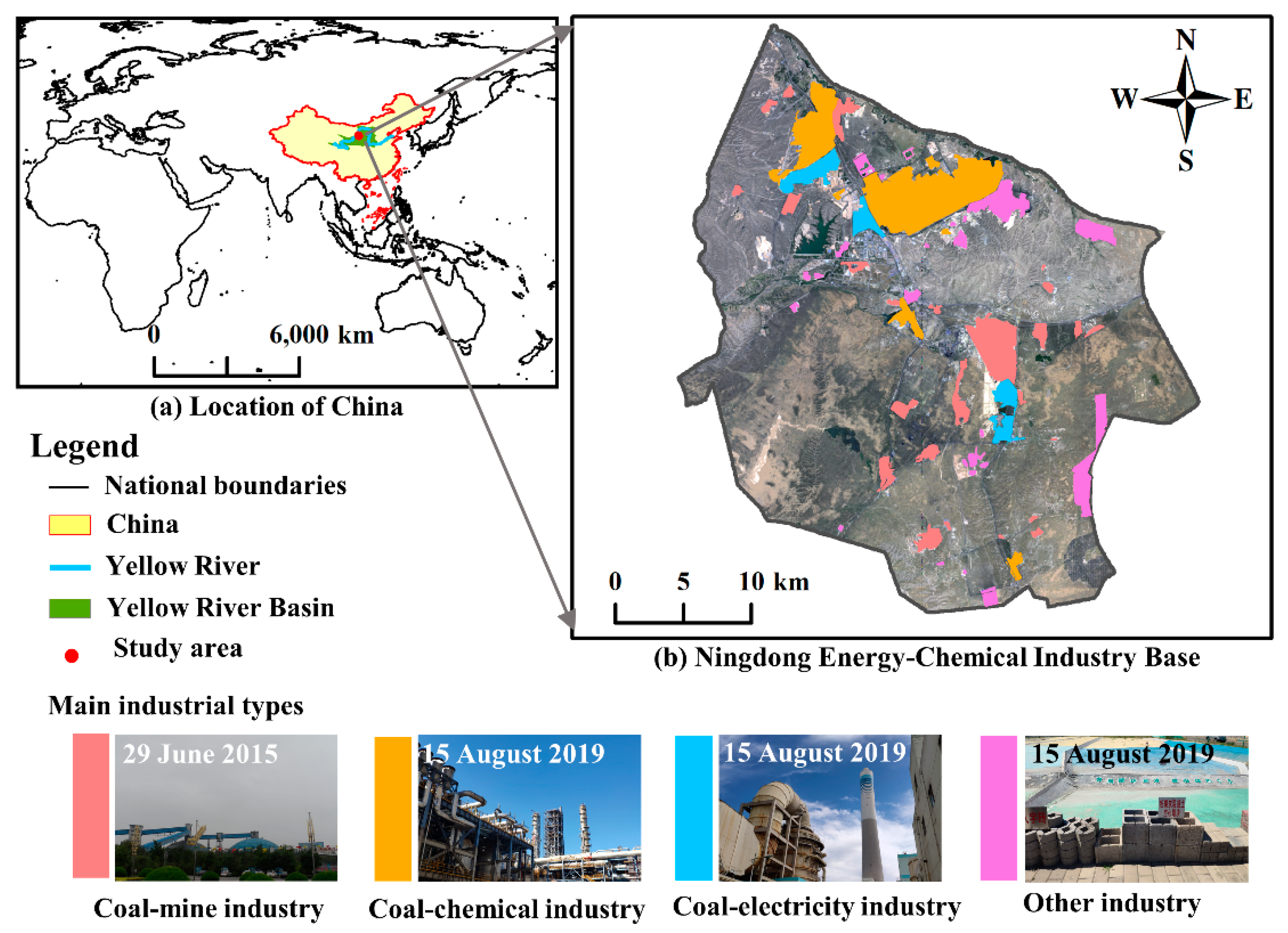
The Ningdong Energy and Chemical Industrial Base (NECIB) is located on the southwest edge of Mu Us Desert and in the middle reaches of the Yellow River Basin (Figure 1). It extends from 106.42° to 106.85° E and from 37.91° to 38.30° N, with a core area of 1000.42 km². Owing to its deep inland location, the NECIB is characterized by a typical temperate continental climate, with an average precipitation of 247.07 mm·a⁻¹ and average evaporation of 1315.50 mm·a⁻¹. The main rivers are the Dahezigou River and Xianjingzigou River, secondary tributaries of the Yellow River [41]. The distribution of cultivated land is scattered and of small scale, mainly planting watermelon, Chinese wolfberry, broccoli, cabbage and tomato.

The study area is close to the Baijitan National Nature Conservation Zone, with the wide distribution of natural vegetation and rich wildlife. Here are some national protected animals (Ciconia nigra, Otis tarda, Aix galericulata, and Cygnus cygnus). The main vegetation types are xerophytic shrubs, semi-shrubs and herbs, such as Caragana korshinskii Kom, Oxytropis aciphylla Ledeb, Agropyron mongolicum Keng, etc. The vegetation coverage is about 10%–45%, with the growth season from June to August [42]. However, the vegetation was easy to destroy but difficult to restore in the Aeolian Sand Area [43], because of the extreme drought and low soil organic matter [44]. Thus, the ecological environment in this region is extremely fragile. Once the eco-environment is destroyed, it will cost these wild animals their habitat.

The NECIB was approved for construction in 2003, and large-scale development began after 2005. Notably, the NECIB has very rich coal resources, with proven coal reserves of 2.73 × 10¹⁰ t·a⁻¹. Together with Yulin in Shaanxi and Ordos in Inner Mongolia, it constitutes China’s Golden Energy Triangle [45]. The industrial cluster’s development has been realized with the three leading industries of coal mining, coal chemical engineering, and coal-fired electricity generation (see in Figure 1). Currently, the NECIB has become a major large-scale coal-based industrial center in China, with a production capacity of 9.16 × 10¹⁰ t·a⁻¹. Moreover, the NECIB has been the major coal-to-chemical industrial base in China, with a coal chemical capacity of 2.25 × 10⁷ t·a⁻¹ [46]. Statistically, the annual increasing rate of the industrial and mining land reached 40.20% between 2008 and 2018 [47]. During the large-scale development period, the construction of coal resources and industrial buildings would inevitably occupy the grassland, forest, shrub, and even arable land. Thus, the NECIB may face severe eco-environmental challenges due to high-intensity coal mining and utilization.

2.2. Data Collection and Preprocessing

The Landsat TM/OLI data were provided by the National Aeronautics and Space Administration (NASA), with a spatial resolution of 30 m. Considering the timing of the large-scale development, we collected the Landsat TM/OLI remote sensing data for the vegetation growing seasons of 2004, 2009, 2014 and 2019 (see

Table 1. Research data.

Data Type	Time	Data ID
Landsat 5 TM	17 August 2004	LT05_L1TP_129034_20040817_20161129_01_T1
Landsat 5 TM	28 June 2009	LT05_L1TP_129034_20090628_20161027_01_T1
Landsat 8 OLI	28 July 2014	LC08_L1TP_129034_20140728_20170420_01_T1
Landsat 8 OLI	26 June 2019	LC08_L1TP_129034_20190726_20190801_01_T1
Digital elevation model data	2009	ASTGTM_N37E106, ASTGTM_N38E106

). The selected remote sensing data were cloud-free, facilitating vegetation dynamic monitoring and landscape classification. Additionally, the digital elevation model (DEM) data were downloaded from the Geospatial Data Cloud of China (GDCC), also with a spatial resolution of 30 m.

The steps of data preprocessing were as follows (see Figure 2): (1) Radiometric calibration, atmospheric correction, and clipping were performed for the Landsat TM/OLI data. An image mosaic was constructed for DEM data. Then, the above data were extracted as a mask, using the boundary of the study area. (2) The land-use/land-cover (LULC) data from 2019 were classified by a support vector machine [48], combined with two field visits (29 June 2015, and 15 August 2019) and high-resolution images from Google Earth. The LULC classifications could be divided into fourteen types, including cultivated land, forest, shrubland, grassland, water, Gobi Desert, sandy land, unused land, residential area, road, coal mine, coal-chemical, and coal-electricity. To improve the accuracy of the results, the Jeffries–Matusita distance parameter was applied to ensure the mean value was greater than 1.9. (3) The Normalized Difference Vegetation Index (NDVI) for 2004, 2009, 2014 and 2019 was calculated based on red and near-infrared bands. Then, the vegetation fractional coverage (VFC) could be estimated using a pixel dichotomy model with a confidence of 5% [49]. (4) The spatial variation trend of VFC from 2004 to 2019 (θ_slope) was analyzed at the pixel scale [50], as shown in Formula (1). Then, an t-test was used to test the significance of θ_slope:

$${\theta }_{\mathrm{slope}}=\frac{1}{5}\times \frac{n\times {\displaystyle \sum _{i=1}^n(i\times VF{C}_{ij})}-{\displaystyle \sum _{i=1}^{n}i}\times {\displaystyle \sum _{i=1}^{n}VF{C}_{ij}}}{n\times {\displaystyle \sum _{i=1}^n{i}^2}-{({\displaystyle \sum _{i=1}^{n}i})}^2}$$

(1)

where i is the vector of the years 2004/2009/2014/2019. The VFC_ij is the VFC value of pixel j in year i. If θ_slope > 0, this indicates that the VFC increased from 2004 to 2019. Otherwise, the trend is decreasing.

2.3. Methodology

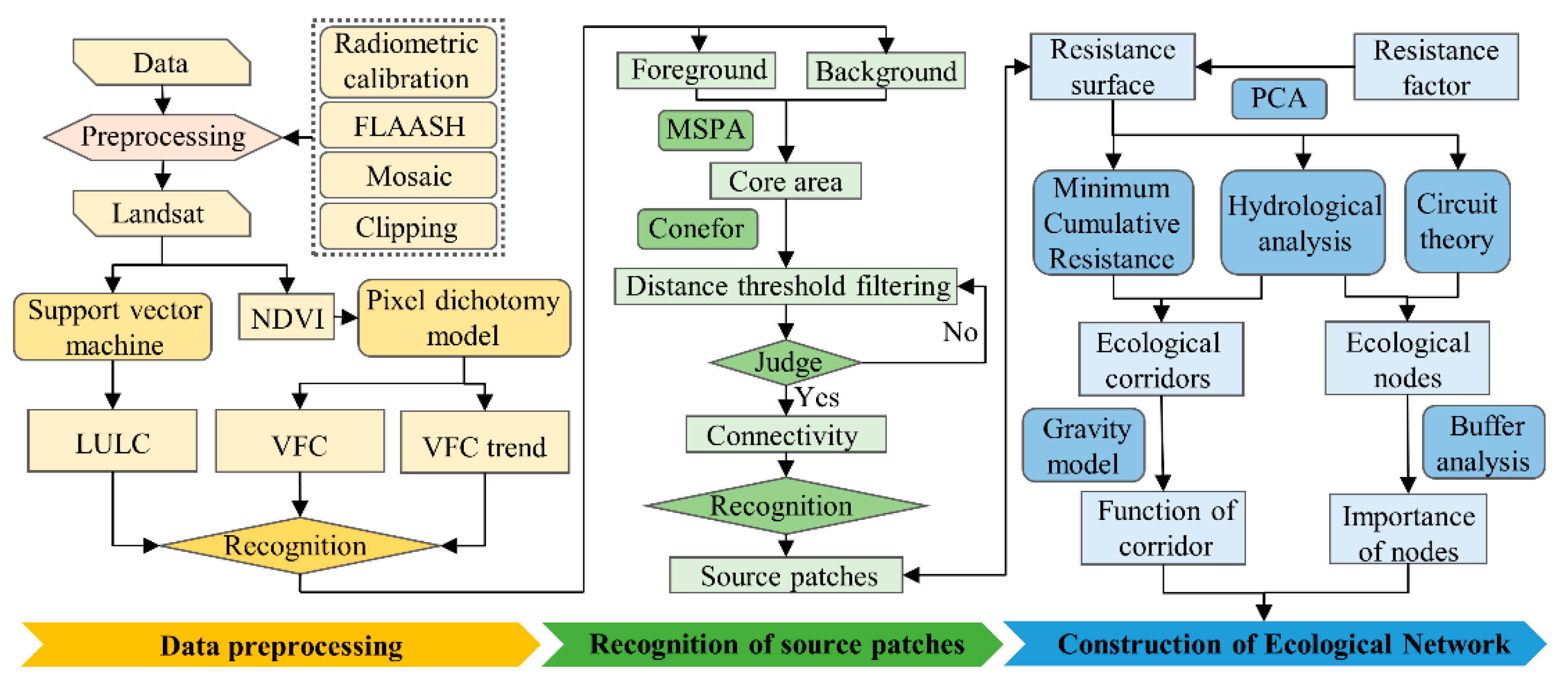
The technology roadmap is shown in Figure 2.

2.3.1. Morphological Spatial Pattern Analysis (MSPA)

The grassland is fragile in the NECIB due to the location in the Aeolian Sand Area. Therefore, it is not advisable to use all grasslands as the foreground data for MSPA [39]. A spatial overlay was applied to extract the grassland with favorable growth in 2019 (VFC ≥ 40%) and significant improvement from 2004 to 2019 (θ_slope > 0, p < 0.1). Then, the forest, the shrubland, and the extracted grassland were merged as foreground data, while other areas were regarded as background data.

The foreground (equal to 2) and background (equal to 1) were converted into binary raster data. Then, raster data were imported into Guidos Toolbox 2.8. Then, foreground connectivity was set to 8 and EdgeWidth to 1 pixel (30 m). Running the Guidos Toolbox 2.8, the foreground data could be divided into seven landscape types, including core; bridge; edge; perforation; islet; loop; and branch [51]. The explanations of different landscape types can be seen in

Table 2. Ecological implications of MSPA classes.

MSPA Type	Ecological Implications
Core	It could be used as the “source patch” of a variety of ecological processes, most of which are forest parks with large patch areas and large forest farms, etc., which are of great significance for species reproduction and biodiversity protection.
Bridge	The narrow and long areas connecting the patches of different core areas, and which have the characteristics of ecological corridors, which are mostly green belts, are conducive to the migration of species and the connection of landscape within the territory.
Edge	The transition zone between the marginal zone of the core area and the peripheral non-green landscape area can reduce the impact brought by the external environment and human disturbance, usually the peripheral forest zone of forest parks and large forest farms.
Perforation	As a transition region, the edge effect also exists between the core patch and its inner non-green space.
Islet	Small patches, which are independent of each other and have low connectivity, are less likely to communicate with other patches in terms of material and energy and are mostly small green spaces in urban or rural areas.
Loop	The internal channel of material and energy exchange in the same core area is the shortcut of material and energy exchange in the core area.
Branch	Only one end is connected to the main patch, mainly an extension of the green space, which is the channel for species diffusion and energy exchange with the peripheral landscape.

.

2.3.2. Identification of Ecological Source Patches

Patch connectivity was regarded as a key indicator to identify source patches [2]. However, the premise of patch connectivity is to determine a distance threshold [10,52]. When the distance between patches is greater than the threshold, it is considered that the patches cannot be connected. Therefore, the core area was extracted from the MSPA analysis, and the patches smaller than 1 ha were removed. Then, a distance gradient was set at every 100 m from 100 to 2000 m, for a total of 20 gradients. Subsequently, the indicators under different thresholds were calculated using Conefor 2.6. The indicators included the connected patches area (CPA), number of patches (NP), number of components (NC), maximum number of patches of components (MNPC), landscape connectivity probability (LCP), integral index of connectivity (IIC) and probability index of connectivity (PC). After determining the distance threshold, the patch connectivity could be evaluated by Conefor 2.6. The patches with the indicators of LCP, IIC, and PC all in the top 30 were then extracted as ecological source patches. These three indicators reflect ecosystem services as well as landscape connectivity [2].

2.3.3. Construction of Ecological Resistance Surface

Eight resistance factors were selected according to a previous study [39,40], as shown in

Table 3. Classification of the ecological resistance factor.

Indicators	Resistance Value
	1	3	5	7	9
Elevation/m	<1250	1250–1300	1300–1350	1350–1400	>1400
Slope/°	<0.5	0.5–2	2–5	5–15	>15
Vegetation fractional coverage	>0.4	0.3–0.4	0.2–0.3	0.1–0.2	<0.1
Landscape type	Forest, shrub, grassland	Cultivated land, water	Gobi, sandy land, unused land	Road, residential area	Coal-mine, coal-chemical, coal- electricity, other industry
Distance from water/m	<500	500–1000	1000–1500	1500–2500	>2500
Distance from road/m	>2000	1500–2000	1000–1500	500–1000	<500
Distance from residential area/m	>2500	1500–2500	1000–1500	500–1000	<500
Distance from industrial site/m	>5000	3000–5000	1500–3000	500–1500	<500

. The weights of the resistance factors were calculated by spatial principal component analysis [23]. Then, the ecological resistance surface was constructed by the grid calculator in ArcGIS 10.6.

2.3.4. Simulation of the Ecological Corridors

Identification of Potential Ecological Corridors

The potential ecological corridors were identified by combining the minimum cumulative resistance (MCR) model with hydrologic analysis (HA). The MCR model is able to simulate the cost of species migrations [29]. The minimum cost paths between each source patch and all other patches were extracted. In addition, repeated paths were eliminated. The MCR model was implemented using the Linkage Mapper, a Python editor-based toolbox for ArcGIS 10.6.

Furthermore, the valley line of the resistance surface was extracted as the ecological corridor layer by HA [53]. The ecological corridors recognized by HA generally appeared to radiate [39,40]. This type of corridor could increase the connection between a source patch and the background matrix and is similar to a branch in MSPA. HA was implemented using ArcGIS 10.6, and its steps were as follows: first, the filling was applied based on the cumulative resistance surface of the distances from source patches. Then, the flow directions and flow rates were calculated. Finally, areas greater than 5500 were extracted as the corridor layer.

The results from the MCR and HA were combined, and then coinciding corridors were removed. Finally, the potential ecological corridors were obtained.

Analysis of the Ecological Corridors

There were two types of potential ecological corridors. One type could connect the source patch through the resistance surface. The other could connect the source patch with the background matrix. For the former, the gravity model (GM) was applied to analyze the interaction intensity [54]. Then, the importance of ecological corridors could be revealed. When the interaction was greater, the resistance between source patches was smaller. The equation for the GM is shown in Formula (2):

$${\mathrm{G}}_{ab}=\frac{L_{\max }^2\times \ln (S_a\times S_b)}{L_{ab}^2\times P_a\times P_b}$$

(2)

where G_ab is the gravity between patch a and b; S_a and S_b are the areas of patches a and b, respectively; P_a and P_b are the resistance value of patches a and b, respectively; L_ab is the cumulative resistance of the corridor from patch a to b, while L_max is the maximum resistance of all corridors.

Furthermore, the difficulty of constructing an ecological corridor was related to the resistance [10]. A greater resistance value represented a more difficult construction for an ecological corridor. A lower value indicated easier corridor construction. Therefore, the minimum cumulative cost distance (MCMD) was calculated, and then the importance of all the potential ecological corridors was analyzed. The potential ecological corridors were divided into five levels (I–V). The higher the corridor level, the more difficult it is to build the corridor.

2.3.5. Simulation of the Ecological Nodes

Recognition of the Potential Ecological Nodes

Ecological nodes can connect adjacent source patches to promote ecological flow [17]. Nodes were usually located in the weak portions of ecological corridors. However, it would be difficult to construct ecological nodes under harsh ecological conditions. Thus, consideration must be given to both the situation regarding the nodes and the connectivity of source patches. HA and circuit theory were used to identify ecological nodes. For HA, the extraction of the ridgeline from the surface was regarded as the maximum cost path that hinders the operation of ecological flow. Thus, the ridgelines of the resistance surface from the HA were extracted. Then, the intersections of the maximum cost paths and the ecological corridors were selected as the ecological nodes.

The “grip” in each minimum cost path was recognized using circuit theory [31]. This was implemented by Pinchpoint Mapper in the Linkage Mapper Toolbox, with the two modes of Pairwise and All-to-one [18]. The “grips” could affect the landscape connectivity of the whole region. Thus, Raster Centrality was selected to extract the “grips” as ecological nodes. Additionally, the barrier was the area which could greatly affect corridor connectivity [31]. If the barrier was restored, it could reduce the least-cost distance (LCD) and improve the connectivity. This step was achieved by Barrier Mapper, a component of the Linkage Mapper toolbox. Thus, the high-value areas were identified as ecological nodes and combined based on the improved score and its percentage to LCD.

The nodes identified by HA and circuit theory were combined, eliminating similar nodes. Then, the potential ecological nodes were obtained.

Analysis of the Ecological Nodes

Determining the location of an ecological node cannot in itself guide future ecological planning. Therefore, it is necessary to further investigate the importance of ecological nodes. The contribution of ecological nodes to landscape connectivity was analyzed by IIC, and then the results were divided into five levels (I–V).

Moreover, it was necessary to analyze the current situation regarding ecological nodes. Therefore, for each node a buffer zone with a radius of 180 m was constructed with the potential ecological node as the center. Then, the buffer area was greater than 10 ha. Then, the buffers were intersected with the 2019 VFC to calculate the average VFC of buffers. The potential ecological nodes were divided into three types, including existing nodes (VFC ≥ 30%), restored nodes (10% < VFC < 30%), and reconstructed nodes (VFC ≤ 10%). Among these, the vegetation condition for a reconstructed node was less favorable than that for a restored node.

3. Results

3.1. Analysis of Landscape Patterns

3.1.1. Extraction of Foreground Data for MSPA

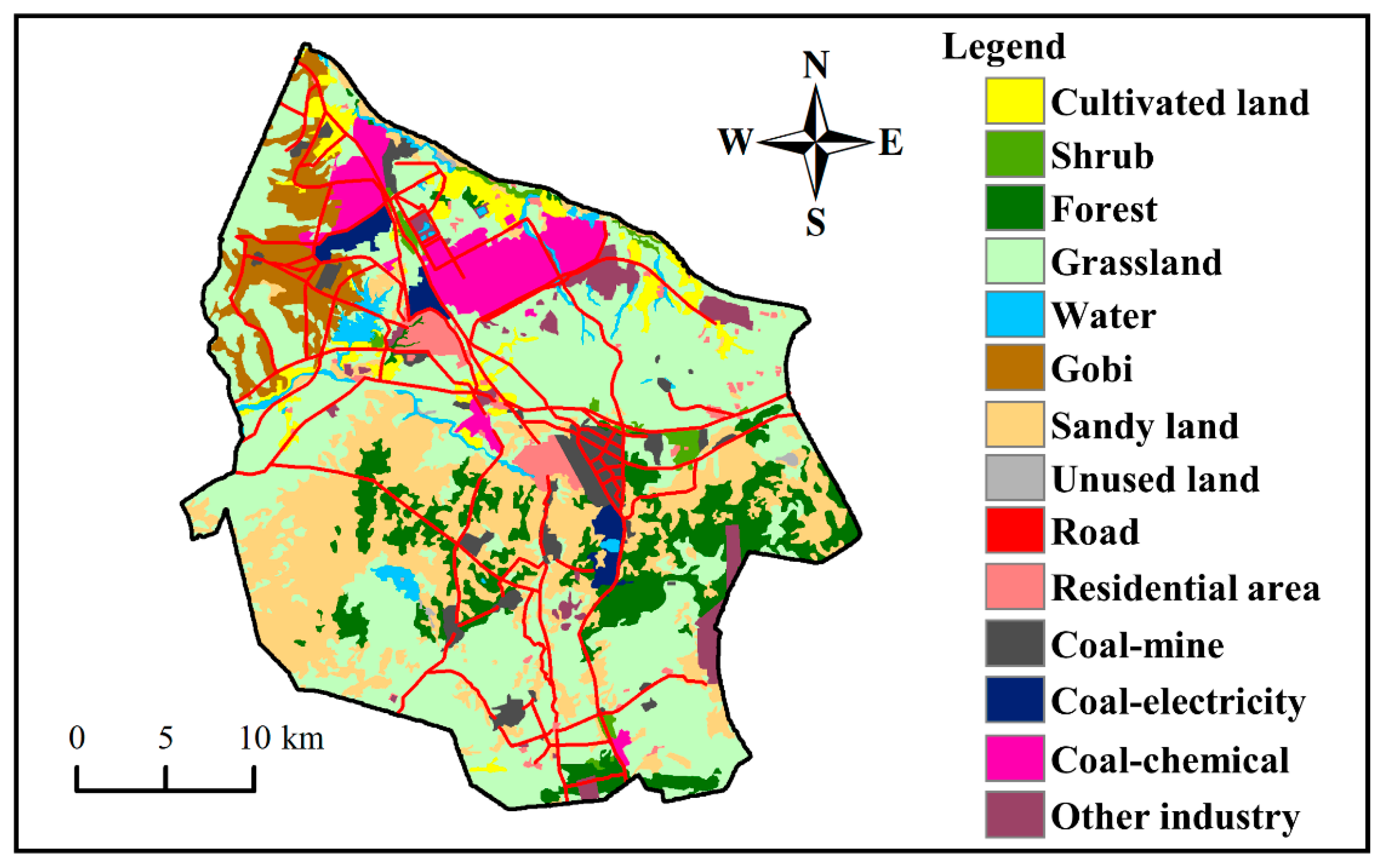
The LULC results are shown in

Table 4. Statistic of land-use/land-cover (LULC) in 2019.

	Area (ha)	Percentage (%)		Area (ha)	Percentage (%)
Cultivated land	3401.28	3.39	Unused land	168.21	0.17
Forest	9884.08	9.84	Residential area	1982.83	1.97
Shrub	1035.47	1.03	Road	2549.63	2.54
Grassland	42,865.00	42.69	Coal-mine	3228.51	3.22
Water	1840.55	1.83	Coal-chemical	5175.85	5.15
Gobi	4693.77	4.67	Coal-electricity	1411.59	1.41
Sandy land	19,562.02	19.48	Other industry	2619.96	2.61

and Figure 3. The study area was dominated by grassland, followed by sand, accounting for 42.69% and 19.48% of the total area, respectively. The areas of unused land and shrubland were the smallest, accounting for 0.17% and 1.03% of the total, respectively. In combination with field investigation, it was determined that some grasslands in the study area were extremely sparse. Thus, the grassland needed to be further extracted.

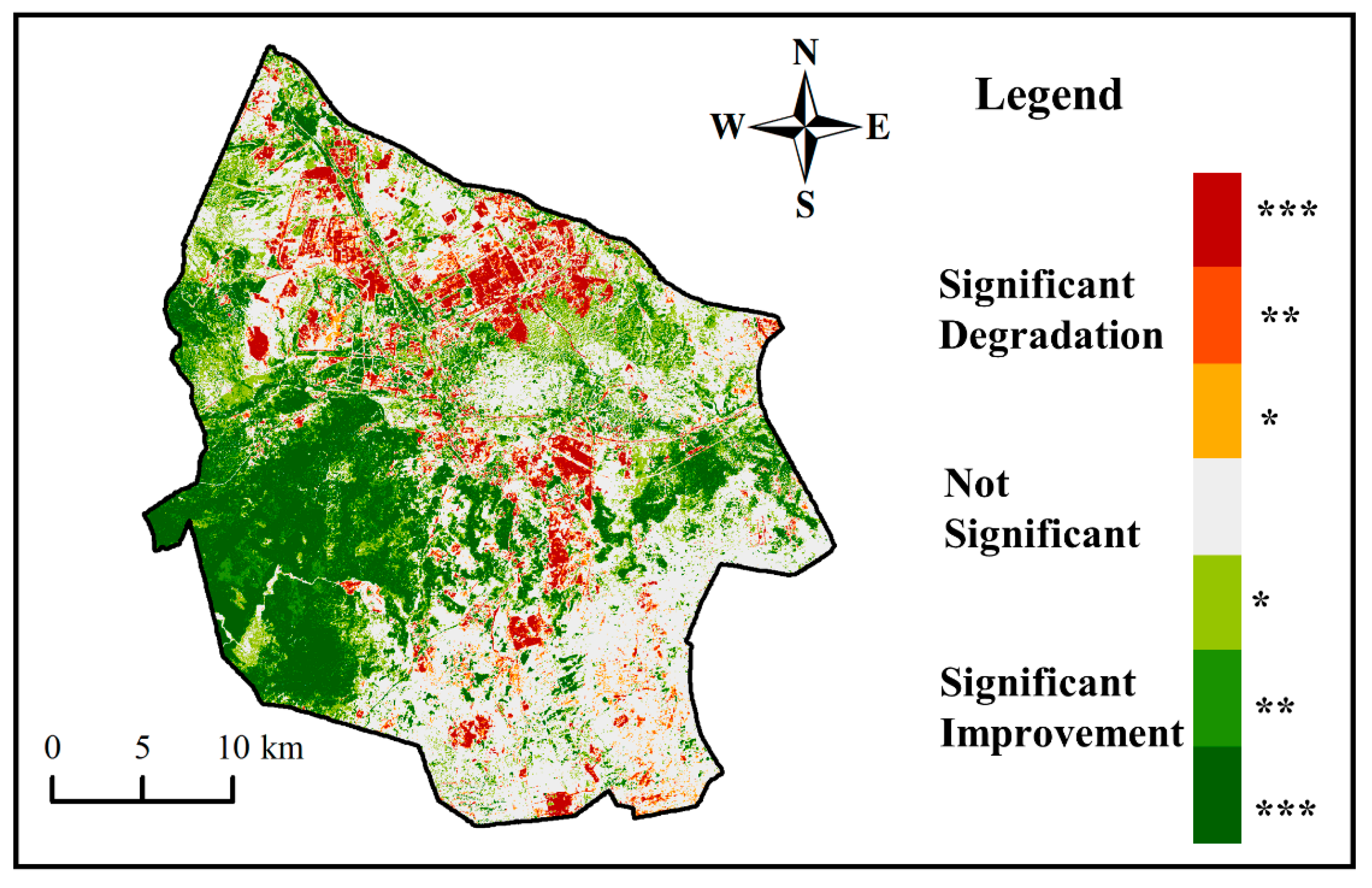
The variation in vegetation fractional coverage (VFC) is shown in Figure 4. From 2004 to 2019, 54.49% of the VFC (54,719.10 ha) changed significantly (p < 0.1). The area of significant improvement was four times as great as the significantly degraded area. The area with improved VFC accounted for 21.20% (21,292.20 ha) and 8.48% (8515.17 ha) at the significance levels of 0.01 and 0.05, respectively. The degraded area accounted for 6.75% (6773.22 ha) and 2.21% (2214.45 ha) at the significance levels of 0.01 and 0.05, respectively. For spatial distribution, the VFC was significantly improved in the southwest (mainly sandy land and grassland). Moreover, the area with significantly degraded VFC was mainly in coal-based industrial sites. Thus, an area of 32,864.49 ha was extracted as the prospective data for MSPA, combined with the results of the LULC and the variation in VFC.

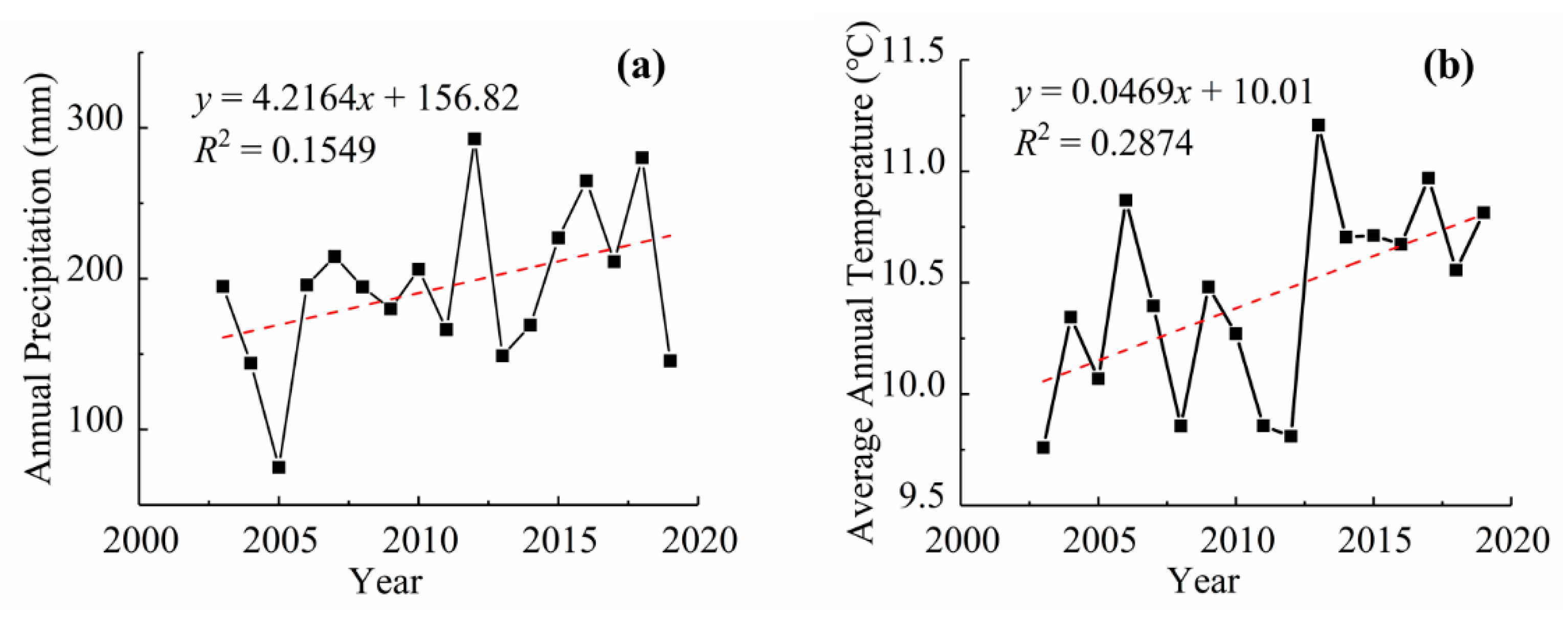
The VFC has improved in the Ningdong Energy and Chemical Industry Base (NECIB), especially in the west. However, is this change caused by climate change or human activity? Due to the lagging effect of climate on vegetation growth [15], 2003 was selected as the initial year. Then, the Lingwu meteorological station was selected, with a distance from the NECIB of only 17.6 km. The temperature and precipitation were recorded from 2003 to 2019. Figure 5 shows that both temperature and precipitation increase linearly, with growth rates of 0.0469 °C·a⁻¹ (R² = 0.2874) and 4.216 mm·a⁻¹ (R² = 0.1549), respectively. The linear fitting effect was not significant, but these data may indicate a trend of warming and becoming wetter. This trend was suitable for the growth of vegetation. Previous studies have shown that the vegetation in northwest China has experienced a trend of “turning green” [50,55], which is consistent with our results.

3.1.2. Recognition of the Core Patches by MSPA

Table 5. Statistics of landscape type based on MSPA.

MSPA Class	Area (ha)	Percentage of the Foreground Data (%)
Core	22,433.30	68.27
Bridge	397.66	1.21
Edge	6980.42	21.24
Perforation	427.24	1.30
Islet	1061.52	3.23
Loop	124.89	0.38
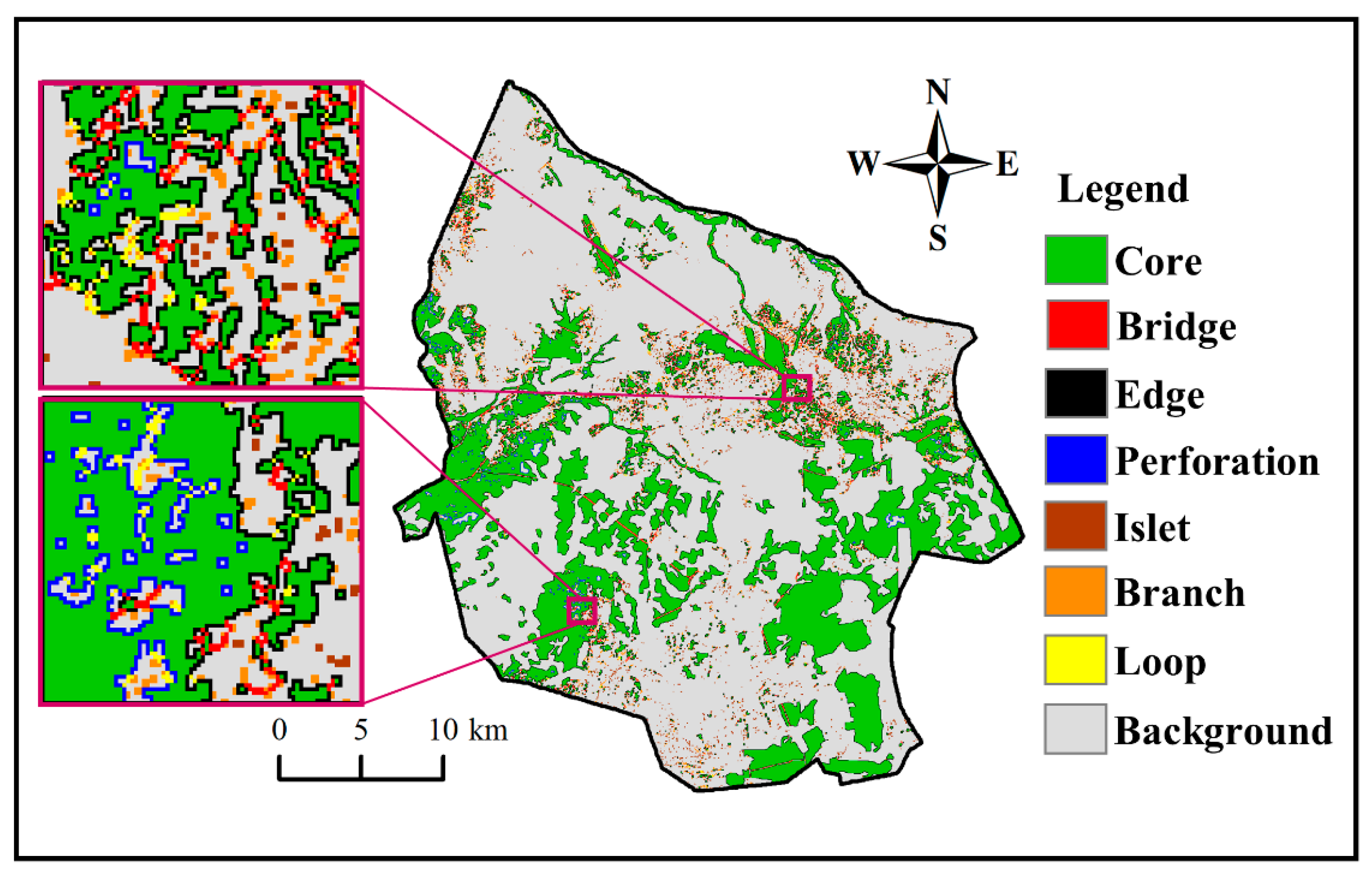
Branch	1439.46	4.38

and Figure 6 show the results of MSPA. The results indicate that the core patches accounted for 68.27% of the foreground data. However, the spatial distribution of core patches was scattered. The larger core patches were mainly distributed in the west and south of the study area. The bridge was a long and narrow area connecting core patches, which could represent a corridor of the ecological network. However, the bridges accounted for only 1.21% of the foreground data. Therefore, the existing ecological corridors cannot meet the requirements for species migrations. The edge and perforation were the outer and inner edge of the patch, accounting for 21.24% and 1.30% of the foreground data, respectively. Both of them were transitional regions between core patches and the background. Generally, the greater the area of edge and perforation, the more scattered the core patches were. Thus, the landscape of the NECIB is seriously fragmented. The branch was the interruption of corridor connection, which had a certain connectivity effect, accounting for 4.38% of the foreground data. The islet was an isolated patch, which could be regarded as a stepping stone for species migration to improve patch connectivity, accounting for 3.23% of the foreground data. The loop was a shortcut for animal movement within the patch, which was beneficial to the migration of species within the same patch, accounting for 3.11% of the foreground data.

3.2. Identifications of the Ecological Source Patches

3.2.1. Determination of the Distance Threshold

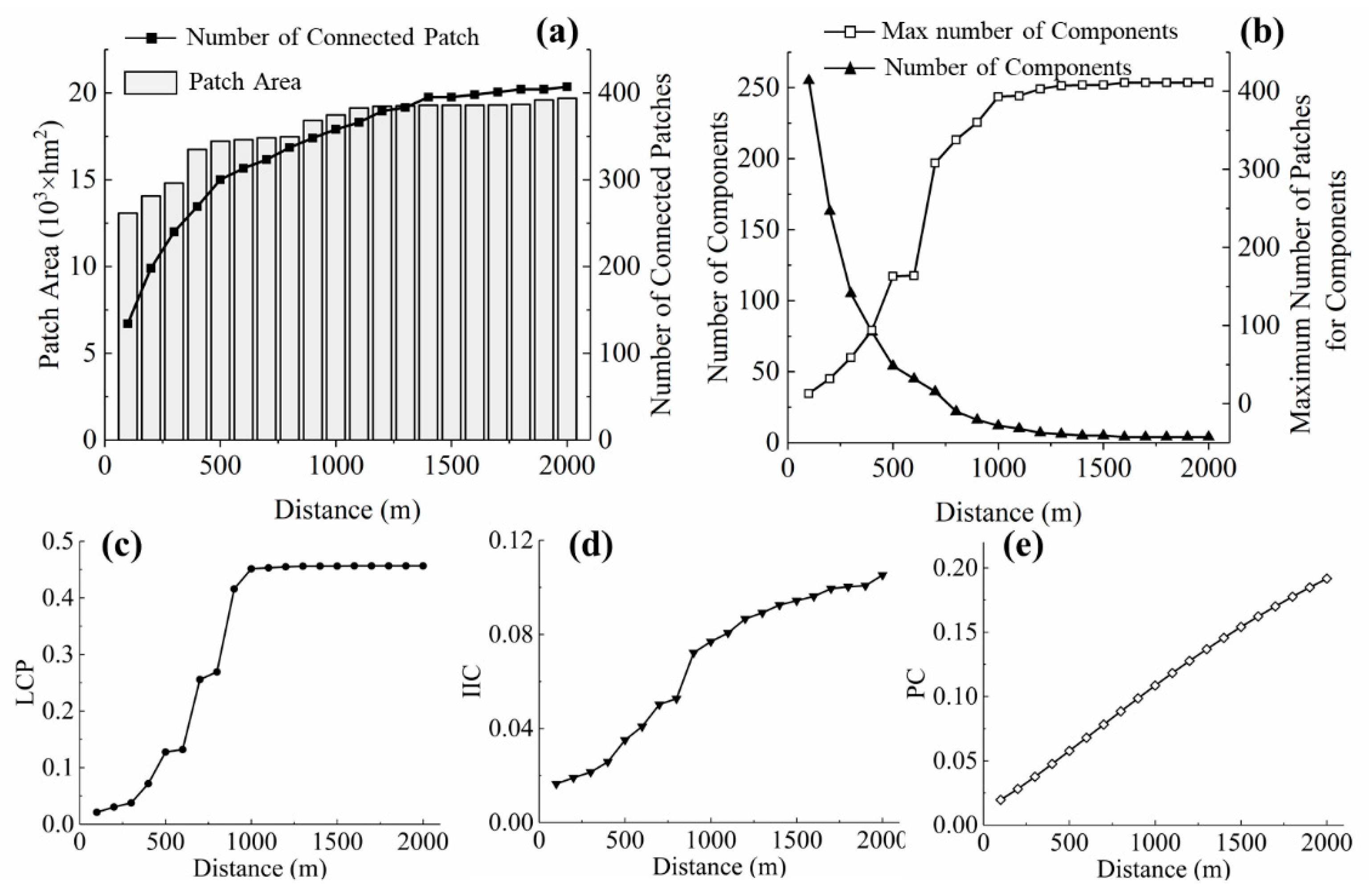
There were 425 core patches after removing the core patches smaller than 1 ha. The results of the distance gradient under different distance thresholds (in the range of 100–2000 m) is shown in Figure 7. Both the connected patch area and the number of patches increased logarithmically with increasing threshold distance, as shown in Figure 7a. When the threshold distance was greater than 800 m, the connected patch area was stable. Figure 7b shows that the maximum number of components increased sharply at 700 m and stabilized at 1200 m, indicating a sensitive range of 700–1200 m. Figure 7c–e shows the variation in LPC, IIC, and PC under different distance thresholds, respectively. Among these, LCP rose steadily (R² = 0.9006) when the distance threshold was less than 800 m. When the distance threshold was greater than 1000 m, variation in LCP was not obvious. Furthermore, IIC and PC increased linearly, with R² values of 0.9403 and 0.9971, respectively. However, IIC changed from 0.0527 to 0.0722 at 900 m. Therefore, the appropriate distance threshold was 900 m from the above analysis.

3.2.2. Identification of the Source Patches

The source patches were essential ecological patches to provide habitat for species. After extracting the patches with values for LCP, IIC, and PC all in the top 30, eighteen patches were recognized as source patches. The total area of source patches was 9455.88 ha.

Table 6. Evaluation of the landscape connectivity index of the ecological source patches.

Patch Number	Area (ha)	LCP	IIC	PC	Patch Number	Area (ha)	LCP	IIC	PC
1	258.75	63.07	30.84	8.46	10	517.68	6.53	10.01	11.70
2	849.24	56.65	24.37	9.71	11	355.23	6.24	4.30	5.37
3	366.39	28.07	18.24	10.21	12	415.80	5.26	4.00	3.51
4	1633.32	23.12	23.76	18.74	13	268.92	3.45	2.70	2.76
5	554.58	22.53	15.84	10.49	14	254.43	3.24	2.85	3.52
6	1119.68	17.02	13.70	13.25	15	220.32	2.81	3.12	4.90
7	969.84	12.04	11.80	11.63	16	154.89	2.48	2.03	2.47
8	963.13	11.96	11.64	18.28	17	176.94	2.26	2.04	2.59
9	203.04	8.87	3.62	2.32	18	173.70	2.22	2.18	3.71

and Figure 7c show the landscape connectivity index of source patches and their distribution, respectively. Table 6 shows that the LCP and IIC of Patch No. 1 exhibited the greatest values, followed by Patch No. 2. Patch No. 1 was located around the Dahezigou River, which is an important river in the study area. The NECIB is vulnerable to the stress of arid climate; thus, the river plays an important role in regulating the eco-environment. Moreover, Patch No. 4 and No. 8 had the greatest values for PC, which was mainly due to the larger areas for Patch No. 4 (1633.32 ha) and Patch No.8 (963.13 ha). Furthermore, little difference was observed among the three connectivity indicators of Patch No. 11–No. 18. This indicates that these source patches contributed similarly to the connectivity. Thus, under the same conditions, the larger the patch was, the greater the habitat suitability and the contribution to ecology.

3.3. Construction of the Ecological Network

3.3.1. Construction of the Ecological Resistance Surface

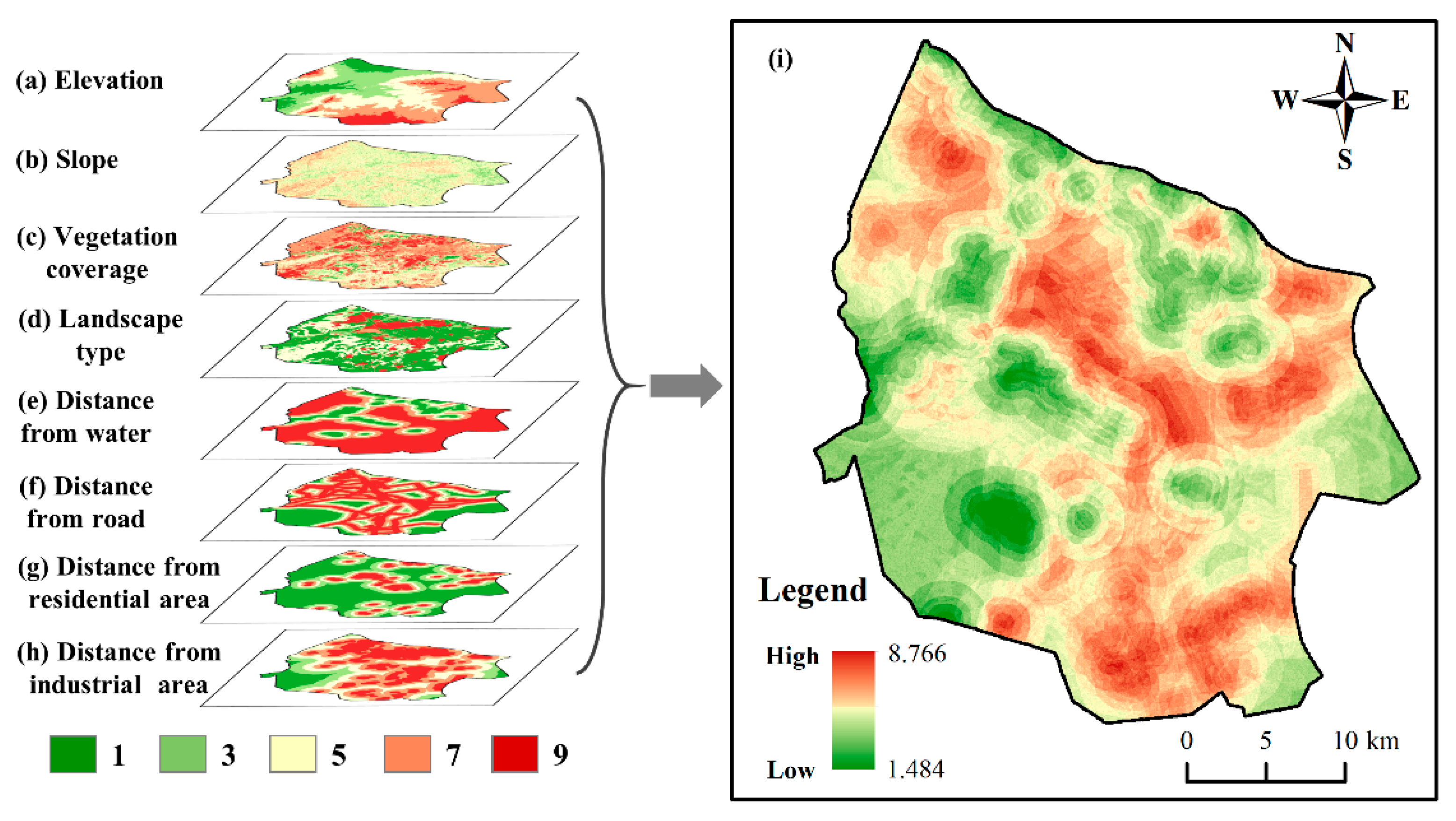
The eigenvalue and percent of eigenvalue of each principal component were obtained by PCA (see

Table 7. Eigenvalues and contribution rates of PCA.

Principal Component	Eigenvalue	Percent of Eigenvalue	Accumulative of Eigenvalue
C1	9.128	30.28	30.28
C2	5.234	17.36	47.65
C3	4.889	16.22	63.87
C4	3.219	10.68	74.54
C5	2.679	8.89	83.43
C6	2.471	8.20	91.63
C7	1.341	4.45	96.08
C8	1.182	3.92	100.00

Note: C represents the principal components, which is also the case below.

). The principal components load matrix and the weights of resistance factors are shown in

Table 8. Principal components load matrix and the weight of resistance factors.

Resistance Factor	Component Matrix								Weight (%)
	C1	C2	C3	C4	C5	C6	C7	C8
Elevation	−0.195	0.318	0.419	0.044	−0.533	0.297	0.491	−0.263	10.59
Slope	−0.052	−0.061	−0.020	−0.038	0.045	0.178	0.447	0.871	3.78
Vegetation Fractional coverage	0.034	−0.303	0.073	0.170	0.210	0.879	−0.219	−0.088	1.13
Landscape type	0.305	−0.726	0.336	0.312	−0.093	−0.267	0.284	−0.097	5.22
Distance from water	−0.305	0.148	0.770	0.062	0.431	−0.161	−0.237	0.144	11.40
Distance from road	0.665	0.185	0.205	−0.531	0.333	0.093	0.252	−0.131	17.86
Distance from residential area	0.368	0.460	−0.096	0.764	0.214	−0.016	0.114	0.019	30.72
Distance from industrial site	0.442	0.098	0.247	−0.009	−0.565	0.030	−0.546	0.341	19.31

. The ecological resistance was obtained from the weighted-overlay resistance factors, as shown in Figure 8. Table 8 indicates high weights for distances from residential areas, industrial sites, and roads. However, the weight of vegetation fractional coverage (VFC) was the lowest, which may reflect the low VFC in the study area.

3.3.2. Analyzation of the Ecological Corridors

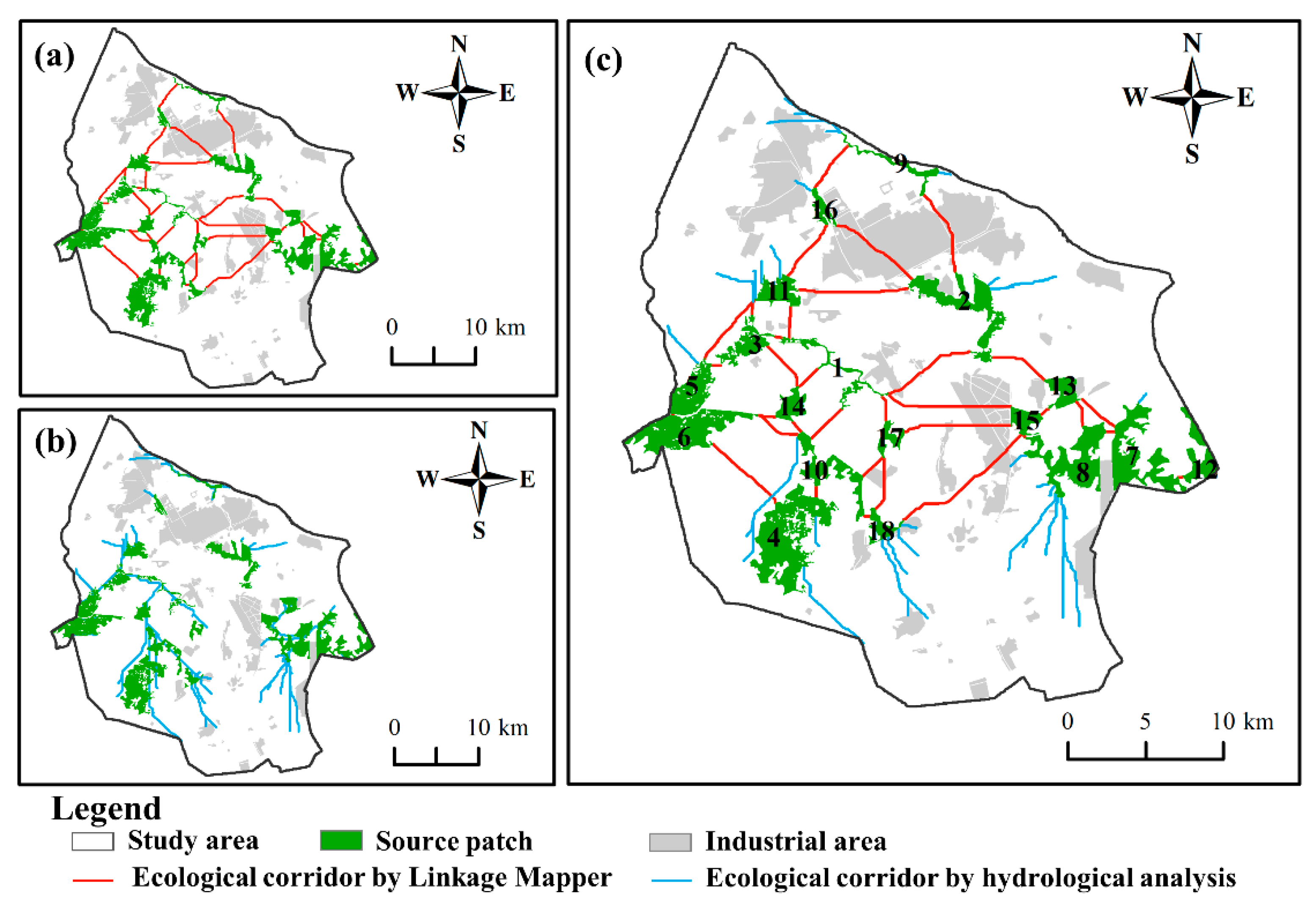
Thirty-four ecological corridors were recognized by Linkage Mapper, as shown in Figure 9a. The ecological corridors were short and dense in the west and southeast, while the corridors were long and sparse in other areas. The total length of the corridors was 104.68 km. The average and the maximum Euclidean distance were 2.86 km and 9.18 km, respectively. The average and the maximum cost-weighted distance were 16.57 km and 53.59 km, respectively.

Figure 9b shows the corridors obtained by hydrological analysis (HA). The results of the combination of the Linkage Mapper and HA can be seen in Figure 9c. There were fifty-eight potential ecological corridors, including twenty-four corridors. If the corridors were only sited between the source patches, there would be no corridors in the south of NECIB. Thus, these corridors have a complementary effect on the ecological corridors, especially in the vicinity of Patches No. 8, No. 9, No. 11, and No. 18. Moreover, these corridors were able to connect the source patches with the surrounding matrix, which could contribute to ecological restoration during a later stage.

The gravity model was applied to analyze the interactions between source patches, as shown in

Table 9. Interaction of ecological corridors between the source patches based on gravity mode.

Patch		Interaction	Patch		Interaction
From	To		From	To
1	2	2.99	5	11	13.47
1	3	897.70	6	10	16.20
1	10	25.73	6	14	111.07
1	11	45.70	7	8	403.93
1	14	198.18	7	12	2267.50
1	15	1.41	7	13	8.36
1	17	75.34	8	13	17.34
2	9	6.09	8	15	5375.54
2	11	2.01	9	16	16.90
2	13	5.12	10	14	176.90
2	16	2.33	10	17	25.14
3	5	858.37	10	18	843.10
3	11	255.76	11	16	15.39
3	14	14.24	13	15	89.47
4	6	11.98	15	17	1.26
4	10	1700.58	15	18	0.93
5	6	26,463.70	17	18	9.16

. At this step, only the corridors between the source patches were analyzed. Table 9 shows the largest interaction (26,463.70), between Patch No. 5 and No. 6, indicating that the greatest connectivity is between these two patches. Furthermore, among the interconnected corridors, the interaction between Patch No. 15 and No. 18 was the least (only 0.45). Such ecological corridors were hard to cross, thus weakening the possibility of material and energy flow. Notably, the connectivity was poor between Patch No. 2 and other patches, with all interactions less than 10.

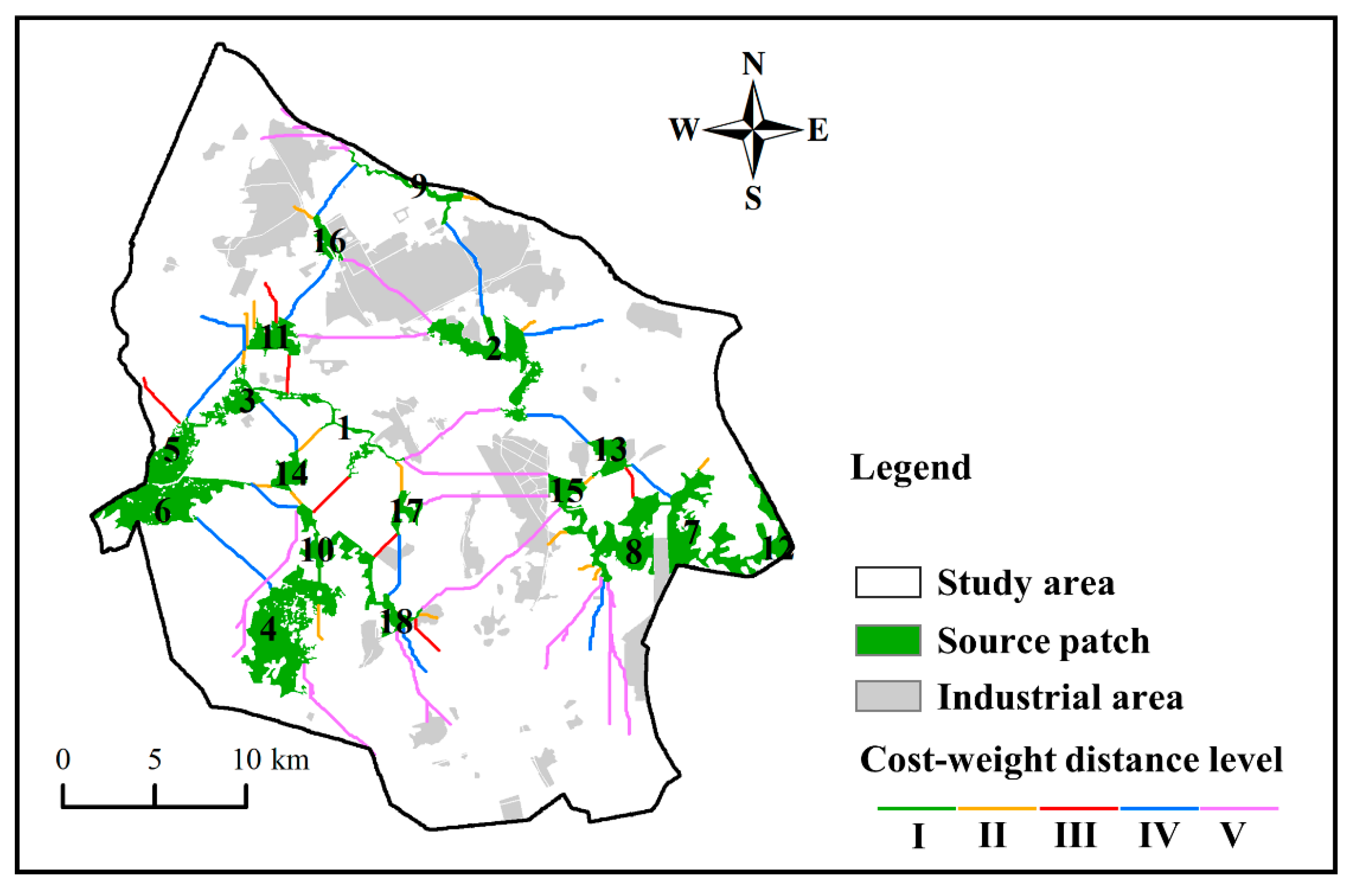
The corridors analyzed by HA were not considered in the gravity model. Thus, the importance of all ecological corridors was further analyzed by cost-weight distance (CWD), as shown in

Table 10. Statistics of the ecological corridors for different level.

Level	Cost-Weight Distance (km)	Number	Total Length (km)
I	<3	8	3.24
II	3–8	17	19.97
III	8–15	7	16.29
IV	15–30	14	57.05
V	> 30	12	102.20

and Figure 10. The CWD classifications of corridors were mainly Level II, Level IV and Level V, accounting for 29.31%, 24.14% and 20.69% of the total number of corridors, respectively. This indicates that the ecological corridors cross the area with greater resistance. In contrast, the number of Level I corridors accounted for 13.79% of the total, while their lengths accounted for only 1.63%. Moreover, there were corridors with a short length but large CWD between Patch No. 6 and No. 10 and between Patch No. 7 and No. 13. These corridors need to cross high resistance areas, such as industrial sites, residential areas, and roads. For the ecological corridors connecting the east and west, only one was Level IV, and the rest were Level V. This revealed the connectivity was low between east and west. Therefore, restoration should be implemented for ecological landscape security patterns in the future.

3.3.3. Analyzation of the Ecological Nodes

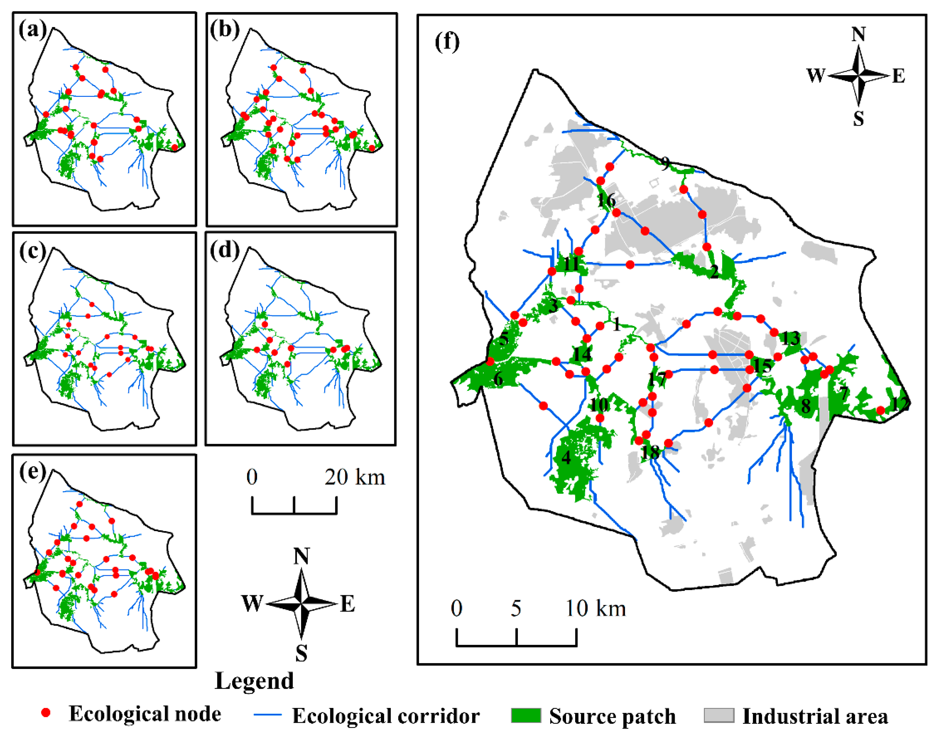
The results of ecological nodes identified by circuit theory are shown in Figure 11a–d. For the pinch points, twenty-one ecological nodes were identified by Pairwise and twenty-seven ecological nodes were identified by All-to-one, as shown in Figure 11a,b, respectively. From the Barrier Mapper, there were sixteen ecological nodes recognized by improved score and nine ecological nodes recognized by improved score percentage, as shown in Figure 11c,d, respectively. Moreover, twenty-five ecological nodes were recognized by HA. The nodes identified by circuit theory were combined with those from HA, and similar nodes were eliminated. Finally, a total of fifty-two ecological nodes were recognized, as shown in Figure 11f.

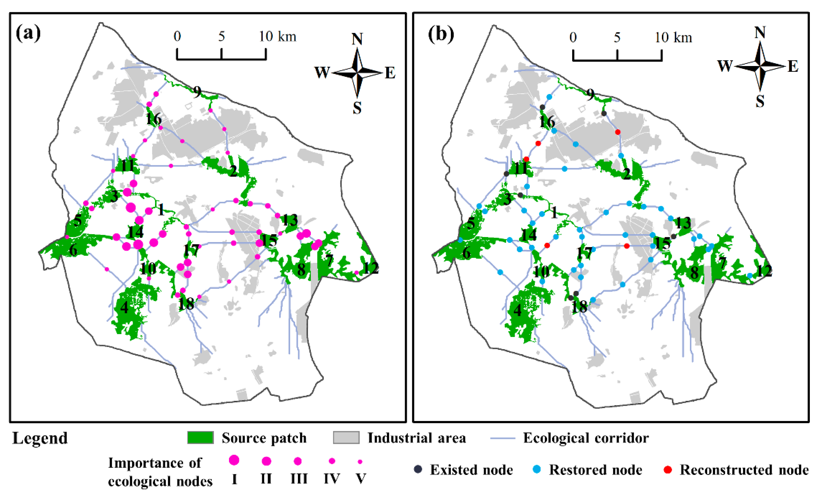
The important levels of ecological nodes were judged according to their contributions to the overall landscape connectivity. The levels were I (IIC > 6.5), II (4.2 < IIC ≤ 6.5), III (3.0 < IIC ≤ 4.2), IV (1.2 < IIC ≤ 3.0), and V (IIC ≤ 1.2), respectively, as shown in Figure 12a and

Table 11. Statistics of the ecological nodes.

Type of Ecological Nodes	Importance Level					Total
	I	II	III	IV	V
Existed	1	0	0	1	3	5
Restored	5	7	6	10	12	40
Reconstruction	1	0	0	3	3	7
Total	7	7	6	14	18	52

. The results showed that the ecological nodes of Level V and VI accounted for the highest proportion of the total, with 34.62% and 26.92%, respectively. The ecological nodes of both I and II accounted for a low proportion of 13.46%. Moreover, the ecological nodes of I and II were mainly concentrated in the grassland and Gobi Desert in the west of the study area. This indicates that the protection of this area may be conducive to the construction of the ecological landscape. Most of the ecological nodes near industrial sites were of Levels III and IV, however, this does not mean that the ecological nodes here are not important. In fact it is quite the opposite: there was poor landscape connectivity near the industrial sites due to a lack of GI patches. Thus, there is an urgent need to undertake greening near the industrial sites.

Table 11 and Figure 12b show that the proportion of ecological nodes that need to be restored was as high as 76.92%. In contrast, the existing ecological nodes account for only 9.62%. This indicates that the ecological network of the NECIB urgently needs to be optimized. In particular, the reconstructed nodes were concentrated in the industrial sites. Therefore, greening in and around the industrial sites is crucial to the overall landscape in the future. Coal-based industries need to balance development and its ecological effects. There were five restored nodes of Level I. Additionally, there was one reconstructed node of Level I, located on the corridor between Patch No. 1 and No. 10. These ecological nodes have great impact in terms of landscape connectivity. Thus, they could be regarded as priorities for establishment in the future.

4. Discussion

4.1. Analysis of Results for Construction of Ecological Networks

The construction of an ecological security pattern could restore biodiversity and maintain the structural process integrity of natural ecosystems [18,28]. Its purpose was to strengthen the spatial pattern of ecosystem function [25] and provide important ecological guarantee for sustainable development [26]. The source patches of NECIB were mainly distributed in the southwest grassland and southeast woodland-shrub ecotone. These areas have high coverage of natural vegetation, rich wildlife resources and a high value of ecosystem services, which are of great significance to regional ecological security. The ecological corridors are distributed in a network among the source patches, connecting the source patches of the study area as a whole. It is worth noting that the Patch No. 2 and No. 17 are very critical, which reduce the length of a single ecological corridor and then reduce the risk of blocking the ecological corridor. Previous studies also found that the landscape heterogeneity of the mining area was unstable and the degree of landscape fragmentation increased [22,56]. Thus, effective measures must be implemented to improve the liquidity and stability of the ecological network. Nevertheless, the proportion of existing ecological nodes was very low, so the stepping stones need to be further improved, especially near the industrial sites.

Notably, the environment is very vulnerable in the Aeolian Sand Area [44]. Even if most areas showed a trend of “greening”, the VFC was degraded in the coal-based industrial sites. Previous study found that about 47.94 km² was transferred from grassland to mining from 2005 to 2018 [47], which was the largest land use transition. Moreover, the Green Infrastructure (GI) of the landscape showed severe fragmentation in MSPA. In addition, the interaction between source patches was low based on gravity analysis. The GI patches were reduced around the coal-based industries, due to the negative environmental effect. Previous studies have found that the mining development activities of large coal bases will have a negative impact on the vegetation and eco-environment, especially in the industrial and mining areas and their surrounding areas [41]. This effect may reduce the possibility of species movement and genetic diversity, and thus reduce the connectivity of the ecosystem [7]. Therefore, ecological restoration should also be accomplished around and inside the industrial sites.

Water resources play a decisive role in vegetation growth in arid areas [49,57], whether it is natural precipitation or surface water [5]. A large source patch area was recognized around Dahezigou River, which corresponds to reality. Therefore, we can further conclude that the Yellow River Protection is beneficial to regional ecological restoration. Moreover, the two largest source patches were located in the southwest (Patch No.4 and No.6), which is highly consistent with the areas of vegetation which have significantly improved in recent years. These findings also demonstrate that vegetation restoration has a significant protective effect on the eco-environment in arid areas.

Generally, resource-based cities are rich in coal resources and hold advantageous locations. Economic production activities often occur in resource-rich areas for the purpose of being close to the producing areas of raw materials and consumer markets. However, in terms of long-term development, the endowment may also become a constraint [11]. Out of the need of political performance assessment, local governments have the incentive to sacrifice the ecological environment for economic development [14]. The processes of resource exploitation, processing and utilization will consume numerous ecological resources, which would increase the ecological security risks, such as the reduction in biodiversity and aggravation of environmental pollution [58]. If not planned and controlled, the excessive expansion of coal-based industrial activities will block the flow of ecological elements, which will not only reduce the supply of ecological products, but also lead to serious consequences such as intergenerational injustice in the distribution of ecological resources.

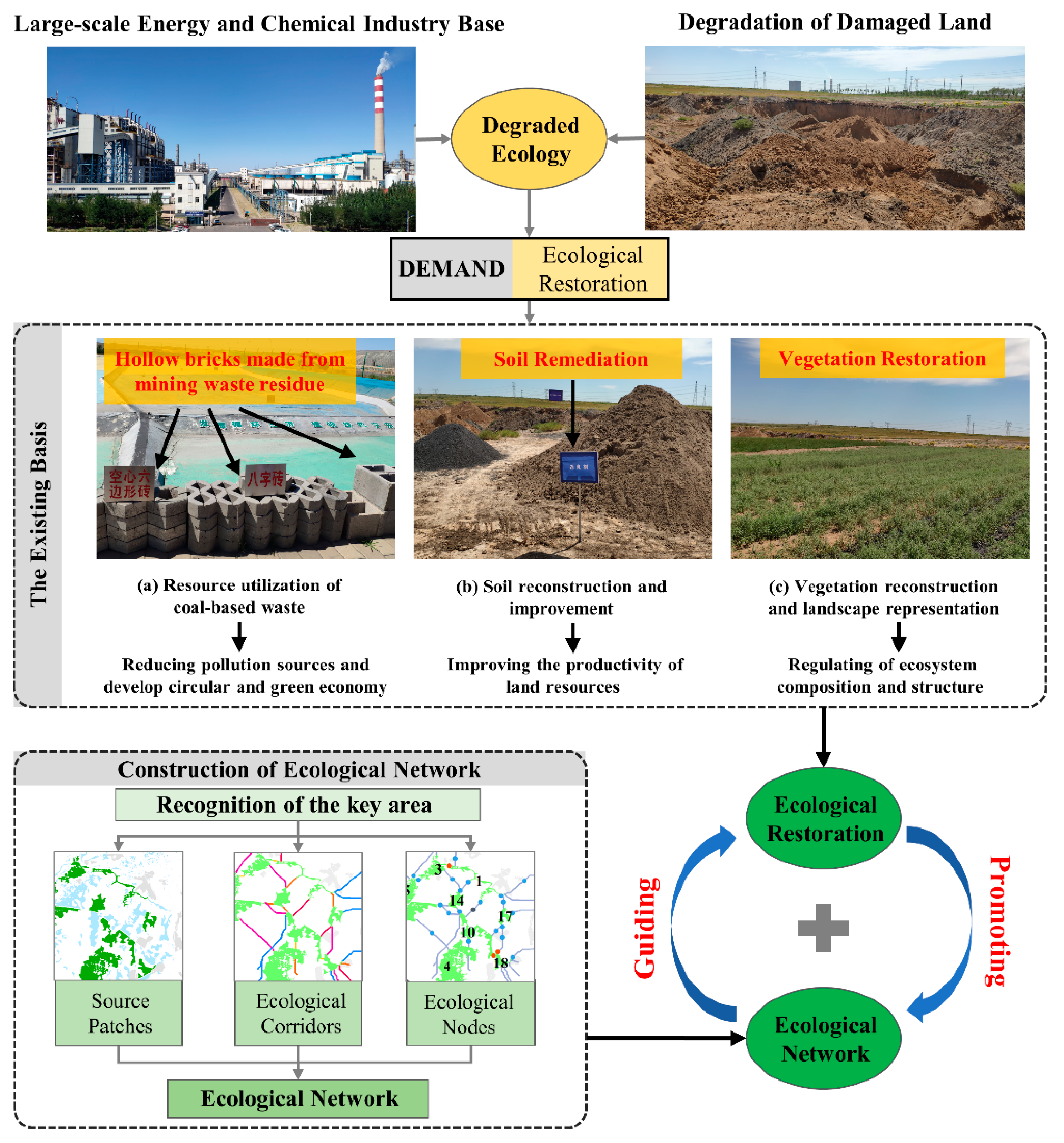
Faced with severe eco-environmental challenges, the local government implemented a series of ecological restoration projects [59]. These projects have achieved effects, including the Project of Ecological Protection along the Yellow River, as well as the Project of Storm Prevention and Sand Immobilization. Additionally, the local coal-industrial enterprises have implemented a series of measures, as shown in Figure 13. Previous studies have noted that the actual cause of environmental pollution is not coal, but the lack of utilization in greenways [60]. For example, hollow bricks could be made from mining waste residue, as shown in Figure 13a. This would not only reduce waste at the source but also promote a circular economy. Moreover, some enterprises have implemented soil amendment and vegetation reconstruction, as shown in Figure 13b,c. The above actions could improve the ecological environment of the region, which is far from sufficient, because the cost of investment must be considered to protect the ecological environment [8]. Thus, the construction of the ecological network is an effective measurement to promote ecological restoration.

4.2. Policy Implications

Eco-environmental problems and resource exploitation tend to be analogous in both developing and developed countries. The development of coal-based industries does not necessarily lead to the deterioration of the ecological environment [53], however, it must focus on balancing the relationship between development and protection [58]. For large energy and chemical bases, ecological security is not only a constraint in short-term development, but also a strategic goal in long-term development. The severe eco-environmental challenges urgently need more appropriate policy guidance in the large energy and chemical bases. Combined with our research, the following policy recommendations are suggested.

4.2.1. Combine Ecological Restoration with the Construction of Ecological Network

The cost of large-scale ecological restoration would be very high. However, if ecological restoration and ecological network construction could be combined, the effectiveness of ecological restoration could be effectively achieved and the cost could also be reduced. Therefore, the ecological network should be completed [17], so as to reduce the negative eco-environmental effects of the coal-based industries. However, it has been hard for nature to form the ecological network, owing to the disturbance of the coal-based industry [39]. Therefore, effective measures should be taken to protect and restore key ecological areas (source patches, ecological corridors, and ecological nodes). Furthermore, the restoration strategies should not only rely on nature. It would be better to combine the artificial induction in the early stage and natural recovery in the later stage.

4.2.2. Improve the Quality and Connectivity of the Source Patch

For ecological patches, priority should be given to select a large area, good quality, high connectivity, or significant improvement in ecological network planning. Some effective measure of ecological protection, restoration and control was needed to improve the habitat quality of these patches. Furthermore, the balance of the spatial distribution for source patches should also be considered to prevent the distance between them being too great. For important ecological patches, efforts should be made to build them into the source patches of large-scale energy and chemical industry base. For example, this study recognized 18 source patches, which were the basis of the ecological network in the NECIB. However, these source patches still showed fragmentation, and effective measures should be taken to restore or merge adjacent source patches.

4.2.3. Restore the Ecological Corridor with High Resistance Value

For ecological corridors, priority should be given to the low values of resistance. Industrial construction, mining activities and traffic roads all have a blocking effect on the ecological network, so these areas with high-value resistance should be avoided as far as possible. When the ecological corridor intersects with them, the blocking effect would hinder the normal migration and spread of organisms, which was not conducive to the flow of matter and energy. Thus, it is suggested that these areas should be properly planned and repaired. In addition, the ecological corridors’ widths could be adjusted based on the local species. If the corridors’ widths do not meet the requirements for species migrations, they would be unable to protect species [20]. For example, this study found that the potential ecological corridors were generally of low grade, high resistance and long length, due to the barrier between coal-based industry and the road. Thus, ecological restoration should be accomplished around and inside the industrial sites and the road, to reduce the resistance.

4.2.4. Reasonable Planning Stepping Stone Restoration

For ecological nodes, priority should be given to high importance and moderate VFC. Ecological nodes were stepping stones for species migration. Increasing the number of stepping stones and decreasing the distance between the stepping stone patches will improve the success rate and survival rate of species during the migration process. Thus, restoration for the priority nodes could promote connectivity and cost savings. For example, this study found that the proportion of ecological nodes that need to be restored was as high as 76.92%, which was extremely difficult to restore. However, there were five restored nodes with a high importance level. Thus, effective measures could be taken to restore these five nodes, which would be of great significance to the construction of the whole ecological network.

4.3. Limitation and Prospects

There are many external disturbances in the large energy and chemical industrial bases, including natural disturbances and human-made disturbances. The human-made disturbances can be further divided into coal-based industrial and other disturbances [49]. However, this study did not identify these disturbance source patches. Thus, further investigation should be conducted to differentiate the environmental effects of different disturbances.

Setting the landscape resistance value was key to the ecological network’s construction, but there is no recognized standard to date. Previously, our research group researched the setting of landscape resistance value of a large-scale coal power base in Inner Mongolia, China [39,40], which was similar to the natural environment and resource endowment of this study area. Therefore, we made a further study with reference to a previous study.

The purpose of the ecological network constructed in this study was to improve the connectivity of habitat patches and the stability of landscape pattern, and to avoid destructive development in the development of energy and chemical industry bases. The source patches were identified based on high VFC and significant improvement. To some extent, these may be representative of most species. However, different species have different requirements for habitat. Thus, we would aim for more specific ecological processes for specific species in the future, which would be more practical.

5. Conclusions

The construction of a large-scale energy and chemical industry base is an important route to promote the integrated and coordinated development of coal and its downstream coal-based industry. Nevertheless, the energy enrichment and ecological fragility are intertwined in semi-arid and arid regions. There is an urgent need to achieve ecological restoration in large-scale energy and chemical bases. Due to the high cost of comprehensive ecological restoration, it is a good way to combine ecological restoration with the construction of an ecological network. Thus, this study took the Ningdong Energy and Chemical Industry Base (NECIB) as a case study. The Landsat TM/OLI data were selected for the vegetation growing seasons in 2004, 2009, 2014 and 2019. Then, the land-use/land-cover (LULC) and vegetation fractional coverage (VFC) were interpreted. The main conclusions are as follows: (1) LULC was dominated by grassland, followed by sand, accounting for 42.69% and 19.48%, respectively. For VFC, the area of significant improvement was four times that of significant degradation. The core patches were recognized by MSPA, with the area of 22,433.30 ha. Then, the landscape connectivity probability (LCP), integral index of connectivity (IIC) and the probability index of connectivity (PC) were applied to evaluate the connectivity of the core patches. A total of 18 patches were extracted as ecological source patches, with a total area of 9455.88 ha; (2) A total of 58 potential ecological corridors were simulated, including 24 corridors analyzed by HA. The ecological corridors had great resistance, so it was difficult to form a natural ecological corridor. Moreover, the connectivity was poor between the east and west of the NECIB; (3) A total of 52 potential ecological nodes were simulated and classified in the NECIB. The high importance nodes were concentrated in the western grassland and Gobi Desert. This indicates that restoration would be conducive to the ecological landscape in this area. Furthermore, five nodes with high importance but low VFC should be given priority in later conservation efforts. Combining the above results, the ecological network optimization of the NECIB was advanced.

References

- Bian, Z.; Yu, H.; Hou, J.; Mu, S. Influencing factors and evaluation of land degradation of 12 coal mine areas in Western China. J. China Coal Soc. 2020, 45, 338–350. [Google Scholar] [CrossRef]
- Wang, S.; Huang, J.; Yu, H.; Ji, C. Recognition of Landscape Key Areas in a Coal Mine Area of a Semi-Arid Steppe in China: A Case Study of Yimin Open-Pit Coal Mine. Sustainability 2020, 12, 2239. [Google Scholar] [CrossRef] [Green Version]
- Hancock, G.R.; Martin Duque, J.F.; Willgoose, G.R. Mining rehabilitation—Using geomorphology to engineer ecologically sustainable landscapes for highly disturbed lands. Ecol. Eng. 2020, 155. [Google Scholar] [CrossRef]
- Novianti, V.; Marrs, R.H.; Choesin, D.N.; Iskandar, D.T.; Suprayogo, D. Natural regeneration on land degraded by coal mining in a tropical climate: Lessons for ecological restoration from Indonesia. Land Degrad. Dev. 2018, 29, 4050–4060. [Google Scholar] [CrossRef]
- Yu, H.; Bian, Z.; Chen, F.; Mu, S. Diagnosis and its regulations for land ecosysten degradation in mining are. Coal Sci. Technol. 2020, 48, 214–223. [Google Scholar] [CrossRef]
- Wu, Z.; Lei, S.; He, B.; Bian, Z.; Wang, Y.; Lu, Q.; Peng, S.; Duo, L. Assessment of Landscape Ecological Health: A Case Study of a Mining City in a Semi-Arid Steppe. Int. J. Environ. Res. Pub. Health 2019, 16, 752. [Google Scholar] [CrossRef] [Green Version]
- Wu, Z.; Lei, S.; Lu, Q.; Bian, Z.; Ge, S. Spatial distribution of the impact of surface mining on the landscape ecological health of semi-arid grasslands. Ecol. Indic. 2020, 111, 105996. [Google Scholar] [CrossRef]
- Yuan, Y.; Zhao, Z.; Niu, S.; Bai, Z. The reclaimed coal mine ecosystem diverges from the surrounding ecosystem and reaches a new self-sustaining state after 20–23 years of succession in the Loess Plateau area, China. Sci. Total Environ. 2020, 727, 138739. [Google Scholar] [CrossRef] [PubMed]
- Bian, Z.; Miao, X.; Lei, S.; Chen, S.; Wang, W.; Struthers, S. The Challenges of Reusing Mining and Mineral-Processing Wastes. Science 2012, 337, 702–703. [Google Scholar] [CrossRef] [PubMed]
- Fu, Y.; Shi, X.; He, J.; Yuan, Y.; Qu, L. Identification and optimization strategy of county ecological security pattern: A case study in the Loess Plateau, China. Ecol. Indic. 2020, 112, 106030. [Google Scholar] [CrossRef]
- Massante, J.C. Mining disaster: Restore habitats now. Nature 2015, 528, 39. [Google Scholar] [CrossRef] [Green Version]
- Yin, D.; Li, X.; Li, G.; Zhang, J.; Yu, H. Spatio-Temporal Evolution of Land Use Transition and Its Eco-Environmental Effects: A Case Study of the Yellow River Basin, China. Land 2020, 9, 514. [Google Scholar] [CrossRef]
- Guo, Y.; Liu, X.; Tsolmon, B.; Chen, J.; Wei, W.; Lei, S.; Yang, J.; Bao, Y. The influence of transplanted trees on soil microbial diversity in coal mine subsidence areas in the Loess Plateau of China. Glob. Ecol. Conserv. 2020, 21, e877. [Google Scholar] [CrossRef]
- Peng, S.; Bi, Y. Strategic consideration and core technology about environmental ecological restoration in coal mine areas in the Yellow River basin of China. J. China Coal Soc. 2020, 45, 1211–1221. [Google Scholar] [CrossRef]
- Zhao, A.; Yu, Q.; Feng, L.; Zhang, A.; Pei, T. Evaluating the cumulative and time-lag effects of drought on grassland vegetation: A case study in the Chinese Loess Plateau. J. Environ. Manag. 2020, 261, 110214. [Google Scholar] [CrossRef]
- Li, P.; Lv, Y.; Zhang, C.; Yun, W.; Yang, J.; Zhu, D. Analysis and Planning of Ecological Networks Based on Kernel Density Estimations for the Beijing-Tianjin-Hebei Region in Northern China. Sustainability 2016, 8, 1094. [Google Scholar] [CrossRef] [Green Version]
- Yu, Q.; Yue, D.; Wang, Y.; Kai, S.; Fang, M.; Ma, H.; Zhang, Q.; Huang, Y. Optimization of ecological node layout and stability analysis of ecological network in desert oasis: A typical case study of ecological fragile zone located at Deng Kou County (Inner Mongolia). Ecol. Indic. 2018, 84, 304–318. [Google Scholar] [CrossRef]
- Peng, J.; Pan, Y.; Liu, Y.; Zhao, H.; Wang, Y. Linking ecological degradation risk to identify ecological security patterns in a rapidly urbanizing landscape. Habitat Int. 2018, 71, 110–124. [Google Scholar] [CrossRef]
- Bascompte, J. Structure and Dynamics of Ecological Networks. Science 2010, 5993, 765–776. [Google Scholar] [CrossRef] [Green Version]
- Gurrutxaga, M.; Lozano, P.J.; Del Barrio, G. GIS-based approach for incorporating the connectivity of ecological networks into regional planning. J. Nat. Conserv. 2010, 18, 318–326. [Google Scholar] [CrossRef]
- Liu, G.; Yang, Z.; Chen, B.; Zhang, L.; Zhang, Y.; Su, M. An Ecological Network Perspective in Improving Reserve Design and Connectivity: A Case Study of Wuyishan Nature Reserve in China. Ecol. Model. 2015, 306, 185–194. [Google Scholar] [CrossRef]
- Xu, W.; Wang, J.; Zhang, M.; Li, S. Construction of landscape ecological network based on landscape ecological risk assessment in a large-scale opencast coal mine area. J. Clean Prod. 2021, 286. [Google Scholar] [CrossRef]
- Xiang, Y.; Meng, J. Research into ecological suitability zoning and expansion patterns in agricultural oases based on the landscape process: A case study in the middle reaches of the Heihe River. Environ. Earth Sci. 2016, 75. [Google Scholar] [CrossRef]
- Kong, F.; Yin, H.; Nakagoshi, N.; Zong, Y. Urban green space network development for biodiversity conservation: Identification based on graph theory and gravity modeling. Landsc. Urban Plan. 2010, 95, 16–27. [Google Scholar] [CrossRef]
- Dai, L.; Liu, Y.; Huang, K. Construction of an ecological security network for waterfront cities based on MCR model and DO index: A case study of Jiujiang city. Acta Geogr. Sin. 2020, 75, 181–196. [Google Scholar]
- Yu, C.; Liu, D.; Feng, R.; Tang, Q.; Guo, C. Construction of ecological security pattern in Northeast China based on MCR model. Acta Ecol. Sin. 2021, 41, 290–301. [Google Scholar]
- Hu, Q.; Chen, S. Optimizing the ecological networks based on the supply and demand of ecosystem services in Xiamen-Zhangzhou-Quanzhou region. J. Nat. Resour. 2021, 36, 342–355. [Google Scholar]
- Guo, R.; Wu, T.; Liu, M.; Huang, M.; Stendardo, L.; Zhang, Y. The Construction and Optimization of Ecological Security Pattern in the Harbin-Changchun Urban Agglomeration, China. Int. J. Environ. Res. Pub. Health 2019, 16, 1190. [Google Scholar] [CrossRef] [Green Version]
- Li, F.; Ye, Y.; Song, B.; Wang, R. Evaluation of urban suitable ecological land based on the minimum cumulative resistance model: A case study from Changzhou, China. Ecol. Model. 2015, 318, 194–203. [Google Scholar] [CrossRef]
- McRae, B.H.; Dickson, B.G.; Keitt, T.H.; Shah, V.B. Using circuit theory to model connectivity in ecology, evolution, and conservation. Ecol. Soc. Am. 2008, 89, 2712–2724. [Google Scholar] [CrossRef]
- Xie, P.; Yang, J.; Wang, H.; Liu, Y.; Liu, Y. A New method of simulating urban ventilation corridors using circuit theory. Sustain. Cities Soc. 2020, 59, 102162. [Google Scholar] [CrossRef]
- Urban, D.K. Landscape connectivity: A graph-theoretic perspective. Ecology 2001, 82, 1205–1218. [Google Scholar] [CrossRef]
- Zhang, L.; Wang, Z.H. Planning an ecological network of Xiamen Island (China) using landscape metrics and network analysis. Landsc. Urban Plan. 2006, 78, 449–456. [Google Scholar] [CrossRef]
- Weber, T.; Sloan, A.; Wolf, S.J. Maryland’s Green Infrastructure Assessment: Development of a comprehensive approach to land conservation. Landsc. Urban Plan. 2006, 77, 94–110. [Google Scholar] [CrossRef]
- Soille, P.; Vogt, P. Morphological segmentation of binary patterns. Pattern Recogn. Lett. 2009, 30, 456–459. [Google Scholar] [CrossRef]
- Shi, F.; Liu, S.; Sun, Y.; An, Y.; Li, M. Ecological network construction of the heterogeneous agro-pastoral areas in the upper Yellow River basin. Agric. Ecosyst. Environ. 2020, 302, 107069. [Google Scholar] [CrossRef]
- Jombart, T.; Dray, S.; Dufour, A. Finding essential scales of spatial variation in ecological data: A multivariate approach. Ecography 2009, 32, 161–168. [Google Scholar] [CrossRef]
- An, Y.; Liu, S.; Sun, Y.; Shi, F.; Beazley, R. Construction and optimization of an ecological network based on morphological spatial pattern analysis and circuit theory. Landsc. Ecol. 2020. [Google Scholar] [CrossRef]
- Zhang, Z.; Du, F.; Huang, J.; Xing, L.; Lei, S. Evaluation of ecological network in surface coal mine: A case study of Shengli open pit mining area. J. China Coal Soc. 2019, 44, 3839–3848. [Google Scholar] [CrossRef]
- Xing, L. Study on Landscape Ecological Network Pattern of Open-Pit Mining Area Based on GIS. Master’s Thesis, China University of Mining and Technology, Xuzhou, China, 2019. [Google Scholar]
- Du, L.; Xu, Y.; Gong, F.; Dan, Y.; Le, W.; Zheng, Q.; Ma, L. Characteristics of vegetation and ecology in Ningdong coal base and the effects of mining activities. Geol. Bull. China 2018, 37, 2215–2223. [Google Scholar]
- Feng, S.; Li, P.; Liu, Z.; Zhang, Y.; Li, Z. Experimental study on pyrolysis characteristic of coking coal from Ningdong coalfield. J. Energy Inst. 2018, 91, 233–239. [Google Scholar] [CrossRef]
- Li, S.; Liang, W.; Fu, B.; Lv, Y.; Fu, S.; Wang, S.; Su, H. Vegetation changes in recent large-scale ecological restoration projects and subsequent impact on water resources in China’s Loess Plateau. Sci. Total Environ. 2016, 569, 1032–1039. [Google Scholar] [CrossRef]
- Du, H.; Xue, X.; Wang, T.; Deng, X. Assessment of wind-erosion risk in the watershed of the Ningxia-Inner Mongolia Reach of the Yellow River, northern China. Aeolian Res. 2015, 17, 193–204. [Google Scholar] [CrossRef]
- Liang, X.; Huang, T.; Lin, S.; Wang, J.; Mo, J.; Gao, H.; Wang, Z.; Li, J.; Lian, L.; Ma, J. Chemical composition and source apportionment of PM1 and PM2.5 in a national coal chemical industrial base of the Golden Energy Triangle, Northwest China. Sci. Total Environ. 2019, 659, 188–199. [Google Scholar] [CrossRef]
- Li, X.; Xiao, R. Analyzing network topological characteristics of eco-industrial parks from the perspective of resilience: A case study. Ecol. Indic. 2017, 74, 403–413. [Google Scholar] [CrossRef]
- El-Hamid, H.T.A.; Caiyong, W.; Yongting, Z. Geospatial analysis of land use driving force in coal mining area: Case study in Ningdong, China. GeoJournal 2019. [Google Scholar] [CrossRef]
- Mi, J.; Yang, Y.; Zhang, S.; An, S.; Hou, H.; Hua, Y.; Chen, F. Tracking the Land Use/Land Cover Change in an Area with Underground Mining and Reforestation via Continuous Landsat Classification. Remote Sens. 2019, 11, 1719. [Google Scholar] [CrossRef] [Green Version]
- Zhang, M.; Wang, J.; Li, S. Tempo-spatial changes and main anthropogenic influence factors of vegetation fractional coverage in a large-scale opencast coal mine area from 1992 to 2015. J. Clean Prod. 2019, 232, 940–952. [Google Scholar] [CrossRef]
- Yuan, J.; Bian, Z.; Yan, Q.; Gu, Z.; Yu, H. An Approach to the Temporal and Spatial Characteristics of Vegetation in the Growing Season in Western China. Remote Sens. 2020, 12, 945. [Google Scholar] [CrossRef] [Green Version]
- Ye, H.; Yang, Z.; Xu, X. Ecological Corridors Analysis Based on MSPA and MCR Model—A Case Study of the Tomur World Natural Heritage Region. Sustainability 2020, 12, 959. [Google Scholar] [CrossRef] [Green Version]
- Qian, D.; Yan, C.; Xing, Z.; Xiu, L. Monitoring coal mine changes and their impact on landscape patterns in an alpine region: A case study of the Muli coal mine in the Qinghai-Tibet Plateau. Environ. Monit. Assess. 2017, 189, 559. [Google Scholar] [CrossRef]
- Su, K.; Yu, Q.; Yue, D.; Zhang, Q.; Yang, L.; Liu, Z.; Niu, T.; Sun, X. Simulation of a forest-grass ecological network in a typical desert oasis based on multiple scenes. Ecol. Model. 2019, 413, 108834. [Google Scholar] [CrossRef]
- Fan, C.; Shen, S.; Wang, S.; She, G.; Wang, X. Research on Urban Land Ecological Suitability Evaluation Based on Gravity-Resistance Model: A Case of Deyang City in China. Procedia Eng. 2011, 21, 676–685. [Google Scholar] [CrossRef] [Green Version]
- Chen, C.; Park, T.; Wang, X.; Piao, S.; Xu, B.; Chaturvedi, R.K.; Fuchs, R.; Brovkin, V.; Ciais, P.; Fensholt, R.; et al. China and India lead in greening of the world through land-use management. Nat. Sustain. 2019, 2, 122–129. [Google Scholar] [CrossRef]
- Zhang, M.; Wang, J.; Li, S.; Feng, D.; Cao, E. Dynamic changes in landscape pattern in a large-scale opencast coal mine area from 1986 to 2015: A complex network approach. Catena 2020, 194. [Google Scholar] [CrossRef]
- Xu, Z.; Lian, J.; Zhang, J.; Bin, L. Investigating and optimizing the water footprint in a typical coal energy and chemical base of China. Sci. Total Environ. 2020, 727, 138781. [Google Scholar] [CrossRef] [PubMed]
- Yu, H.; Bian, Z.; Chen, F. Dynamic Mechanism of Land Ecological Restoration in Mining Area: Based on Land Degradation Neutrality (LDN) Framework. China Land Sci. 2020, 34, 86–95. [Google Scholar]
- Wang, Y.; Xiao, Y.; Xie, G.; Xu, J. Sand-fixing function of the grassland ecosystem in Ningxia based on the revised wind erosion model. Resour. Sci. 2019, 41, 980–991. [Google Scholar] [CrossRef]
- Hu, Z.; Zhu, Q.; Liu, X.; Li, Y. Preparation of topsoil alternatives for open-pit coal mines in the Hulunbuir grassland area, China. Appl. Soil. Ecol. 2020, 147, 103431. [Google Scholar] [CrossRef]
Figure 1.
(a,b) Location of the study area and the main industrial types.
Figure 2.
Technical flow chart. The meanings of the abbreviations are as follows: FLAASH is the fast line-of-sight atmospheric analysis of spectral hypercubes; NDVI is the normalized difference vegetation index; LULC is land-use/land-cover; VFC is the vegetation fractional coverage; MSPA is morphological spatial pattern analysis; PCA is principal component analysis.
Figure 3.
Land-use/land-cover (LULC) in 2019.
Figure 4.
Spatial variation in vegetation fractional coverage (VFC) from 2004 to 2019. Significant at * p < 0.1, ** p < 0.05, and, *** p < 0.01, respectively.
Figure 5.
Annual precipitation (a) and average annual temperature (b) in Lingwu County from 2003 to 2019.
Figure 6.
Distribution of landscape types based on MSPA.
Figure 7.
The variation in landscape connectivity indices under different distance thresholds using Conefor 2.6: (a) connected patch area and number of patches; (b) number of components and maximum number of patches for components; (c) landscape connectivity probability (LCP); (d) integral index of connectivity (IIC); and (e) probability index of connectivity (PC).
Figure 8.
Landscape ecological resistance surface.
Figure 9.
Distribution of ecological corridors: (a) identified by Linkage Mapper; (b) identified by hydrological analysis (HA); and (c) the potential ecological corridors combining results from the Linkage Mapper and HA.
Figure 10.
Distribution of the ecological corridors for different levels.
Figure 11.
Distribution of the ecological nodes: (a–d) are the ecological nodes by circuit theory. (a) pinch points from Pairwise; (b) pinch points from All-to-one; (c) nodes recognized by Barrier Mapper based on improved scores; (d) nodes recognized by Barrier Mapper based on improved score percentages; (e) ecological nodes recognized by hydrological analysis; and (f) combined results of hydrological analysis and circuit theory.
Figure 12.
Importance and classification of ecological nodes in the Ningdong Energy and Chemical Industrial Base (NECIB): (a) different importance levels of ecological nodes by IIC; and (b) different types of ecological nodes by VFC.
Figure 13.
Combine the construction of ecological network with ecological restoration.