


List of symbols and units

1. Introduction
The major portion of the East Antarctic (EA) ice sheet (Fig. 1) has been dynamically stable for many millennia, as currently shown by the 800 000-year-old-basal ice at Dome C (Jouzel and others, Reference Jouzel2007) and the million-year ice at marginal blue ice areas (Sinisalo and Moore, Reference Sinisalo and Moore2010). Surviving through major cycles of climate change with cold-glacial and warm inter-glacial periods, changes in the marginal extent and the inland thickness of the EA ice sheet have been small compared to changes in the West Antarctic (WA) and Greenland ice sheets (e.g. Denton and Hughes, Reference Denton and Hughes1981; Denton, Reference Denton2011; Mackintosh and others, Reference Mackintosh2011; Bentley and others, Reference Bentley2014; Pollard and others, Reference Pollard, Gomez and DeConto2017). In contrast to EA, much of WA is grounded 1000 m below sea level, has a maximum surface elevation of 2000 m (only half of EA), may be susceptible to dynamic instabilities, and has a more uncertain and complicated long-term history, including its major retreat after the Last Glacial Maximum (LGM) and partial re-advance of the grounding lines during the Holocene (Kingslake and others, Reference Kingslake2018).

Fig. 1. Antarctic ice sheet regions and drainage systems. East Antarctica (EA) is divided into EA1 (DS2 to DS11) and EA2 (DS12 to DS17). The Antarctic Peninsula (AP) includes DS24–27. West Antarctica (WA) is divided into WA1 (Pine Island Glacier DS22, Thwaites and Smith Glaciers DS21, and the coastal DS20) and WA2 (inland DS1, DS18, and DS19 and coastal DS23). Includes grounded ice within ice shelves and contiguous islands.
In general, variations in the total mass (M(t)) of the Antarctic ice sheet (AIS) are the sum of short-term (≲decades) accumulation-driven variations (M a(t)) in the surface mass balance and sub-decadal to millennial dynamic variations (M d(t)). Dynamic changes in ice velocity occur for various reasons such as changes in ice-shelf back-pressure, basal sliding or long-term changes in accumulation rate that cause changes in ice thickness and surface slope that drive long-term changes in velocity.
The mass balance of the EA ice sheet has been significantly affected by long-term changes in snowfall, as shown by the 50–200% increases in accumulation beginning after the LGM ~15 ka BP and continuing through the Holocene as derived from ice cores (Siegert, Reference Siegert2003). That continuing long-term accumulation increase was a key factor supporting the interpretation of the 1.59 cm a−1 thickening of the EA ice sheet, derived from both ERS1/2 (1992–2001) and ICESat (2003–08) altimetry measurements, as persistent long-term dynamic thickening with a dynamic mass gain of 147 Gt a−1 (Zwally and others, Reference Zwally2015). This Holocene ice growth in EA is also consistent with the evidence of Holocene glacier advances from the EA ice sheet through the Transantarctic mountains into the Dry Valleys (Stuiver and others, Reference Stuiver, Denton, Hughes and Fastook1981; Denton and Wilson, Reference Denton and Wilson1982). In contrast, the most marked area of contemporary dynamic changes and coastal ice thinning in EA is on Totten glacier at 116°E (Zwally and others, Reference Zwally2005; Pritchard and others, Reference Pritchard, Arthern, Vaughan and Edwards2009; Li and others, Reference Li, Rignot, Mouginot and Scheuchl2016).
As analysis methodologies for both satellite altimetry and gravimetry have advanced in recent years, the largest remaining difference in mass-balance estimates (Shepherd and others, Reference Shepherd2012, Reference Shepherd2018; Hanna and others, Reference Hanna2013; Zwally and others, Reference Zwally2015; Hanna and others, Reference Hanna2020) has been for the EA ice sheet (Fig. 1). The agreement has been generally better in WA. However, the behavior in the coastal portion (WA1) is dominated by dynamic losses and is markedly different from the mostly inland portion (WA2) that has significant dynamic thickening, of which some is similar to the thickening in EA (Zwally and others, Reference Zwally2015).
The mass balances of both EA and WA are also significantly affected by decadal variations in accumulation such as those between the 1992–2001 ERS1/2 period and the 2003–08 ICESat period: (a) the regional shift in EA of +21 Gt a−1 in EA1 and −21 Gt a−1 in EA2, and (b) an increase in WA snowfall that offset 50% of the increased losses of 66 Gt a−1 from enhanced dynamic thinning on accelerating outlet glaciers in WA1 and the Antarctic Peninsula (AP) (Zwally and others, Reference Zwally2015). Therefore, determination of both the short-term accumulation-driven and the long-term dynamic-driven components of ice-sheet mass balance is critically important for understanding the causes of changes on various time scales and the ice sheet's ongoing- and future-contributions to global sea-level change.
In their Figure 3, Hanna and others (Reference Hanna2020) show the variation in the estimates of Antarctic dM/dt from 1990 to 2018 obtained by the three principal methods (altimetry, gravimetry and input–output method), which is updated from a similar figure in Hanna and others (Reference Hanna2013). For EA, those reviews, as well as the multi-investigator results (Shepherd and others, Reference Shepherd2018) from the second Ice Sheet Mass Balance Inter-comparison Exercise (IMBIE), clearly show outliers on both sides of the means, indicating that disparate estimates (~100 Gt a−1) of the EA mass balance have not been properly resolved.
In this paper, we focus first on the mass balance of the EA and WA ice sheets and on resolving the differences between gravimetry-based and altimetry-based estimates of the balance during the 2003–08 period of overlapping measurements. Our method is motivated by indications that a principal residual uncertainty in prior estimates was due to errors in their respective corrections (GIAcor and dB cor) for changes in the volume and mass of the Earth underneath the ice caused by changes in the glacial loading on the crust and mantle (Fig. 2). The process of adjusting to changes in the glacial loading is commonly called Glacial Isostatic Adjustment (GIA). For the case of full isostatic (hydrostatic) equilibrium, the vertical motion of the bedrock (dB/dt) would be zero. However, under large ice masses, the long-term isostatic state is never actually fully reached as the glacial loading continually changes and the underlying fluid mantle hydrodynamically adjusts to the changes in the gravitational forcing.

Fig. 2. Ice sheet of thickness, T, lying on Earth's crust and underlying fluid mantle. For long-term isostatic equilibrium (~10 ka) with constant ice thickness the depth of the depression would be D ≈ ρ ice /ρ mantle × T, which is 600 m for T = 3000 m and ρ mantle = 4.5, and the dB/dt would be zero. As the glacial loading, T(t), on the Earth's crust continually changes, the underlying viscous mantle hydrodynamically adjusts over centuries to millennia. Illustration is for an increasing ice thickness that induces a downward motion of the crust (i.e. dB/dt < 0), outward mantle flow and mantle thinning. For this case, the GRACE senses the gravitational changes of the increasing ice mass minus the decreasing mantle mass (ΔM) under the satellite. ICESat senses the increase in ice thickness minus the downward motion of the crust and mantle caused by the change in mantle volume (ΔV).
We use the results of three GIA models (Whitehouse and others, Reference Whitehouse, Bentley, Milne, King and Thomas2012; Ivins and others, Reference Ivins2013; Argus and others, Reference Argus, Peltier, Drummond and Moore2014; Peltier, Reference Peltier2014), which are dynamic models of the Earth's crust (lithosphere) and the underlying fluid mantle forced by changes in the glacial loading. The models provide the gravitational signal for GIAcor and the vertical motion of the bedrock for calculation of dB cor. We derive the respective sensitivities (S g and S a) of the GIAcor and dB cor to the bedrock motion from the models. We then use S g and S a to derive the bedrock motion (i.e. δB 0) needed to match the mass changes during 2003–2008 from GRACE and ICESat without any GIAcor and dB cor applied, and alternatively the adjustments (i.e. δB adj) to the modeled bedrock motions with model-based GIAcor and dB cor applied. We then use the adjusted GIAcor to extend the mass-change time series using GRACE gravimetry data through to 2016.
The introduction in Whitehouse and others (Reference Whitehouse, Bentley, Milne, King and Thomas2012) presents a thorough review of prior calculations of GIA corrections applied to GRACE data and the effect of residual model errors on the estimates of ice mass balance. Constraints on the models are provided by the measurements of relative sea level and GPS measurements of crustal motion, which are also used for the estimation of residual errors (Whitehouse and others, Reference Whitehouse, Bentley, Milne, King and Thomas2012). In EA where fewer constraining measurements have been made, especially inland on the vast area of the ice sheet, the errors are likely to be largest. The review by Hanna and others (Reference Hanna2013) noted: ‘… several key challenges remain …, changes in ice (sheet) extent and thickness during the past millennium are poorly known, and typically not included in GIA models, despite the fact that they can dominate the present-day rebound signal, especially in regions of low mantle viscosity’.
In order to further establish the validity of the ICESat 2003–08 elevation and mass changes as the baseline for reconciling the GRACE GIAcor and the ICESat dB cor, we review the methods and corrections employed in our data analysis and derivation of elevation and mass changes in section 5 and the Appendix. We first review the compatibility and validity of our elevation and mass changes derived from ERS1/2 for 1992–2001 and ICESat 2003–08 as presented in Zwally and others (Reference Zwally2015), showing how those results agreed with other studies. We include a new comparison of the corrected dH/dt derived from ERS1/2 and ICESat with the corrected dH/dt derived from Envisat radar altimetry from Flament and Rémy (Reference Flament and Rémy2012). That comparison shows the essential agreement of the dH/dt measured over EA by the four satellites with differing instrumentation over 19 years from 1992 through 2010 at the level of a few mm a−1. Flament and Rémy (Reference Flament and Rémy2012) developed unique methods for correction of the highly-variable (seasonally and interannually) sub-surface radar penetration not used in other Envisat nor CryoSat radar altimeter studies, which as detailed in the Appendix is a principal reason why other studies have differed from ours.
Overall, as GIA modeling has advanced in recent years, the results remain fundamentally dependent on knowledge of the history of the glacial loading, especially in the vast inland parts of the AIS where physical constraints from measurements are not feasible and knowledge of loading history is limited. Furthermore, there has been a lag in model incorporation of new information on the glacial loading as it becomes available from paleo-rates of ice accumulation derived from ice cores (e.g. Siegert, Reference Siegert2003; Siegert and Payne, Reference Siegert and Payne2004) and radar layering (Vieli and others, Reference Vieli, Siegert and Payne2004), from our altimetry results and conclusions on inland ice growth (Zwally and others, Reference Zwally2005), and from information on Antarctic glacial geology and ice modeling (e.g. Stuiver and others, Reference Stuiver, Denton, Hughes and Fastook1981; Denton and Wilson, Reference Denton and Wilson1982; Bradley and others, Reference Bradley, Hindmarsh, Whitehouse, Bentley and King2015; Pollard and others, Reference Pollard, Gomez and DeConto2017; Kingslake and others, Reference Kingslake2018). In our conclusions, we discuss how our regional values of δB 0 are consistent with current knowledge and interpretation of the history of glacial loading and with new findings of a lower mantle viscosity in WA by Barletta and others (Reference Barletta2018).
We apply the derived dB cor corrections to the ERS1/2 results for 1992–2001 as well as the ICESat results for 2003–2009, and the corresponding GIAcor to the GRACE results for 2003 through to the beginning of 2016, thereby showing the mass-balance variations for all of the AIS and by regions over 24 years.
2. Summary of approach to reconciling altimetry and gravimetry mass-changes
In the same way that satellite gravimetry measures changes in the ice mass on the Earth's crust and altimetry measures changes in the ice volume, the respective measurements include the effects of ongoing changes in the mass and volume (ΔM, ΔV) of the Earth under the ice. The fundamental concept of our approach for resolving the difference between GRACE- and ICESat-based estimates of ice mass changes is based on the realization that the respective mass and volume corrections are for the ΔM and ΔV of the same underlying material. The changing Earth material is illustrated schematically in Figure 2 as a distinct element (ΔM, ΔV) of the mantle, even though the actual material involved is spatially distributed in three dimensions within the mantle and may include elastic deformation of the crust. Furthermore, the required mass and volume corrections are both provided by the same dynamical models of the motion within the Earth caused by changes in the glacial loading (e.g. either Whitehouse, Ivins or Peltier GIA models). These models calculate the change in gravity caused by the ΔM and the vertical motion of the bedrock, dB/dt, caused by the ΔV. Although our concept emphasizes the mass and volume changes of the fluid mantle that force motion of the crust, it also includes the more rapid elastic deformation of the crust noted in Section 3, as do our bedrock motions calculated for the matching of GRACE and ICESat mass changes in Section 6.
For gravimetry, the correction (GIAcor) is for the rate of change in gravity caused by the ΔM/Δt mass-change underneath the ice in units of the rate of mass change, which is essentially

where ρ earth is the relative density of mantle material involved in the ΔM/Δt change. For altimetry, the correction (dB cor) to the mass changes calculated from changes in ice-sheet surface elevation (dH/dt) is made for the vertical motion of the bedrock (dB/dt) caused by the ΔV/Δt. The dB cor is equal to ρ ice ΔV/Δt, where ρ ice is the relative density of ice, 0.91, that is typical of the density in deep ice cores rather than 0.917. (Throughout the paper, we use densities relative to that of water, 1 g cm−3, so densities are used as dimensionless quantities, being 1 for water). The use of ρ ice is appropriate, because basal motion displaces solid ice and does not affect the density nor volume of the firn column. GIAcor and dB cor are used here as rates of mass change per unit area, so using ΔV/Δt = dB/dt × area, the GIAcor and dB cor per unit area are:


where dB/dt is positive upward. The GIAcor and dB cor corrections are always subtracted from the uncorrected observations. For example, positive values of GIAcor and dB cor corrections reduce mass gains or increase mass losses.
Although GIAcor and dB cor are defined as rates of mass change per unit area, as are the dM/dt rates of mass change, both are often written in units of rates of vertical mass change such as mm w.e. a−1 without an explicitly associated area that requires multiplication by an area to get mass change per unit area. Examples are the modeled GIA given in units of mm w.e. a−1 in Figure 3 and the cm w.e. a−1 scale for the dM/dt in Figure 14, for which the implicit area for the latter is 1.0 cm2 and the rate of mass change is 1.0 g a−1 cm−2 that is equivalent to 0.1 Gt a−1 (100 km)−2 as shown in the color scale in Figure 16 (and S2). We also use units of mm w.e. a−1 for the average values of GIAcor over specific regional areas as in column 2 of Table 1 with the regional rates of mass change in units of Gt a−1 in column 3.

Fig. 3. Glacial Isostatic Adjustment (GIA) in mm w.e. a−1, basal uplift (dB/dt) in mm a−1, and RatioG/db equal to GIA/(0.91 × dB/dt) derived by three Earth models labeled Ivins, Whitehouse and Peltier (Whitehouse and others, Reference Whitehouse, Bentley, Milne, King and Thomas2012; Ivins and others, Reference Ivins2013; Peltier, Reference Peltier2014). Subsidence rate from glacial loading in the central part of EA ice sheet is largest in Whitehouse model and smallest in Ivins.
Table 1. Glacial Isostatic Adjustment (GIA) and uplift (dB/dt) from Ivins, Whitehouse and Peltier Earth models

GIA (mm w.e. a−1) and dB/dt (mm a−1) are regional-average rates and GIAcor (Gt a−1) and dB cor(Gt a−1) = 0.91 dB/dt are area-integrated regional rates of the corrections. S g and S a sensitivities and RatioG/dB are also regional averages defined in the text.
a See text about the calculation of S g and RatioG/dB.
We define RatioG/dB as

the gravimetry sensitivity (S g)md to bedrock motion as

where the subscript (md) indicates the GIA model used (Iv, Pe or Wh), and the altimetry sensitivity (S a) to bedrock motion as

The units of dB/dt are mm a−1, the units of GIAcor and dB cor are Gt a−1, the units of S g and S a are both Gt a−1/mm a−1, and

We include minus signs in the sensitivity definitions so a positive change in dB/dt (i.e. more uplift) causes the derived mass change to decrease and a negative change (i.e. more subsidence) causes it to increase. Whereas S a is a geometric factor depending only on ρ ice, area and the dB/dt from the GIA models, the S g includes additional dependencies on the characteristics of the models.
S g and S a provide a straightforward linear relation for reconciling the differences in the GRACE and ICESat mass estimates by calculating the rate of uplift or subsidence (δB 0-md) needed to provide the GIAcor and dB cor corrections that bring the respective mass estimates into full agreement (i.e. [(dM/dt)GRACE]eq = [(dM/dt)ICESat]eq). The required uplift or subsidence, δB 0−md, relative to zero is given by:

where [(dM/dt)GRACE]0 and [(dM/dt)ICESat]0 are the respective GRACE and ICESat measurements with zero GIAcor and zero dB cor applied as indicated by the subscript (0). The second subscript (md) indicates the GIA model used to calculate the gravity sensitivity, i.e. (S g)Iv, (S g)Wh or (S g)Pe for Ivins, Whitehouse or Peltier model. For example, δB 0-Iv indicates that (Sg)Iv derived from the Ivins model of GIA and dB/dt was used with no dB cor nor GIAcor applied to the measured dM/dt.
The required uplift or subsidence (δB adj-md) is also calculated relative to the GIA modeled

where md is either Iv, Pe or Wh. The resulting GRACE and ICESat equalized mass changes using either δB 0-md or δB adj-md are denoted

As shown in Section 6, the differences among the three (dM/dt)eq-md are small, and therefore the mass-change adjustment is largely independent of the particular GIA model used, even though relative differences among the modeled dB/dt are large.
Previously, Zwally and others (Reference Zwally2015) used a preliminary estimate of RatioG/dB = 6 with S g = −55.7 Gt mm−1 and S a = −9.3 Gt mm−1 for EA. For EA, the uncorrected GRACE and ICESat dM/dt of 61 Gt a−1 and 136 t a−1, respectively, came into agreement at 150 Gt a−1 after adjusting the uplift by δB adj-Ivx = −1.6 mm a−1. (The subscript Ivx indicates that some parameters of the Ivins model run previously used for the calculation of dB cor were not exactly the same as those for GIAcor and S g.)
The RatioG/dB also provides a basis for estimating the incremental long-term effect (δB′) on the rate of bedrock motion of a long-term dynamic ice thickening, (dH d/dt)obs, using

Eqn (9) is based on the hypothesis that the long-term dynamic response of the Earth's mantle to a continued long-term ice loading produces a corresponding downward flow of mantle material with mass and ice-volume changes in the ratio of RatioG/dB with respect to the ice loading. As noted in the introduction, the 15.9 mm a−1 ice thickening observed in EA was interpreted as commencing at the beginning of the Holocene. Therefore, the corresponding estimated change in the long-term compensation rate was δB′ = −15.9/6 = −2.65 mm a−1. This δB′ is 1.7 times larger than the δB adj-Ivx = −1.6 mm a−1 required for the mass-matching adjustment, which suggests that some but not all of the observed thickening may have been included in the model's ice loading history. In the following, we derive more accurate values of RatioG/dB and related parameters from the results of the three GIA models.
Finally, we note that our approach to resolving differences in the GRACE- and ICESat-based estimates of ice mass changes is fundamentally different from those proposed or applied by others. Wahr and others (Reference Wahr, Wingham and Bentley2000) proposed combining GLAS (ICESat) and GRACE measurements to slightly reduce the post-glacial rebound error in the GLAS mass-balance estimates. Shepherd and others (Reference Shepherd2012) ‘reconciled’ estimates of mass balance by taking the mean of selected estimates from three techniques (altimetry, gravimetry and input–output method). Riva and others (Reference Riva2009) combined ICESat and GRACE measurements using: (1) for ICESat data a surface snow density, ρ surf, ranging from 0.32 to 0.45 for some ice areas, an intermediate (between firn and ice) density of 0.60 in other ice areas, and the density of pure ice (0.92) in areas where rapid changes in ice velocity have been documented; and (2) for GRACE data a rock density, ρ rock, under grounded ice ranging from 3.4 to 4.0 in order to obtain the GIA impact on GRACE-derived estimates of mass balance of 100 ± 67 Gt a−1. Martin-Español and others (Reference Martin-Español, Bamber and Zammit-Mangion2017) performed a statistical analysis combining satellite altimetry, gravimetry and GPS with prior assumptions characterizing the underlying geophysical processes and concluded that gains in EA are smaller than losses in WA, although we show in the Appendix that their use of a single density for estimating mass changes from elevation changes is not correct.
3. GIA and bedrock vertical motion (dB/dt)
The fundamental physical process involved in GIA is glacial loading/unloading that bends the Earth's crust and forces 3-D viscous flow in the underlying fluid mantle, as illustrated in Figure 2. Part of the elastic bending is relatively rapid, for example, as shown by GPS-measured seasonal vertical motions of the crust in response to the seasonal cycle of summer surface melting and water runoff from the ablation zone of Greenland (Nielsen and others, Reference Nielsen2013). In contrast, another part of the crustal bending occurs along with the viscous flow of the mantle with uplift and subsidence rates that decay exponentially, with response times depending on the viscosity, following changes in the glacial loading or unloading. For example, adjustments following the relatively abrupt demise of the Laurentide ice sheet ~10 K years ago are continuing with current uplift rates on the order of +15 mm a−1 in central Canada (Peltier, Reference Peltier2004) and subsidence rates south of the former ice sheet, for example, −1.7 mm a−1 in the Chesapeake Bay region (DeJong and others, Reference DeJong2015) from the hinge effect in the crustal bending. However, the response time strongly depends on the viscosity of the mantle, which is a principal parameter typically varied in the models to improve agreement with the constraining information available on uplift rates. For example, the analysis of Barletta and others (Reference Barletta2018) indicated a lower viscosity and faster uplift rate in the Amundsen Sea Embayment (ASE) in WA than previous studies. As noted in Barletta and others (Reference Barletta2018), viscosities ~1018–1019 Pa s correspond to decadal to centennial response times as shown in the AP (Nield and others, Reference Nield2014), in Southern Patagonia (Richter and others, Reference Richter2016) and in Alaska (Larsen and others, Reference Larsen, Motyka, Freymueller, Echelmeyer and Ivins2005). Viscosities ~1020–1021 Pa s correspond to millennial response time scales and are typically used in global and Antarctic GIA models (Whitehouse and others, Reference Whitehouse, Bentley, Milne, King and Thomas2012; Ivins and others, Reference Ivins2013; Argus and others, Reference Argus, Peltier, Drummond and Moore2014; Peltier, Reference Peltier2014).
The density of the mantle ranges from ~3.4 to 4.4 in the upper mantle and from 4.4 to 5.6 in the lower mantle (e.g. Robinson, Reference Robinson2011). In contrast, the density of the crust is generally lighter, ranging from 2.2 to 2.9 similar to surface rocks such as granite, basalt and quartz. A somewhat common misconception is that the material involved in the GIA correction has the density of the surface or crustal rocks (e.g. ρ ≥ 2.7 in Zwally and Giovinetto, Reference Zwally and Giovinetto2011), rather than primarily the greater densities of the underlying fluid mantle.
In our analysis, we use the GIA and dB/dt uplift results provided by three GIA models labeled Ivins, Whitehouse and Peltier with the maps of the modeled data given in Figure 3. GIA models may have variations in model characteristics, parameters (e.g. mantle viscosities, mantle densities and crustal thickness), ice-loading histories, and their use of GPS and other data to constrain the model results, details of which are given in the references. In EA, the models generally show crustal subsidence in the central portions of the ice sheet with an uplift in the coastal regions and along the boundary with WA. This pattern of subsidence and uplift implies a radial outflow of mantle material from the central region, and inflow at the outer regions from both the central region and southward from the Southern Ocean. Over many millennia, the spatial and temporal variability of the glacial loading history produces a complex 3-D flow of the mantle, which on a continental scale at any given time can have flow in multiple directions at different depths with regions of convergence and divergence. During the short decadal times of satellite measurements, temporal variations in the mantle flow and the resulting uplift and subsidence rates are small.
The regional average values of GIAcor (mm w.e. a−1) and dB/dt (mm a−1) for the Ivins, Whitehouse and Peltier models are given in Table 1 along with the regional GIAcor (Gt a−1) and dB cor (Gt a−1) mass corrections. [Note: total regional values are calculated as GIAcor (Gt a−1) = GIAcorr (mm w.e. a−1) area (km2) 10−6 and dB cor (Gt a−1) = 0.91 dB/dt (mm a−1) area (km2) 10−6.] The GIAcorr and dB cor are both positive for positive dB/dt (i.e. uplift) and are subtracted from the measured gravity and altimetry mass changes (i.e. conventional usage). For the three models, the GIAcor and dB cor mass corrections for EA and WA are mostly comparable in magnitude, with the smaller area of WA (18% as large as EA) offset by its seven times greater average uplift.
For EA, the area of subsidence inland is largest in the Whitehouse model (Fig. 3) with subsidence more than −2 mm a−1 in three locations and an area-averaged value of −0.19 mm a−1 (subsidence), in contrast to average uplift rates of 0.42 mm a−1 for Ivins and 0.60 mm a−1 for Peltier (Table 1). For EA, the Ivins average GIAcor is 1.9 mm w.e. a−1 uplift and the regional dM/dt adjustment is −19.9 Gt a−1. The GIAcor is largest for the Peltier model at 3.1 mm w.e. a−1 with a regional dM/dt adjustment of −31.5 Gt a−1. For Whitehouse, the average GIAcorr is −0.9 mm w.e. a−1 with a regional dM/dt adjustment of +8.8 Gt a−1. Differences among the modeled GIAcorr are as large as 40 Gt a−1 between the Peltier and Whitehouse models for EA (mostly EA1), 15 Gt a−1 between Peltier and Ivins for WA (mostly WA2), and 45 Gt a−1 between Peltier and Whitehouse for AIS.
The spatial variations of the model results and variations among the models are also illustrated by the profiles of GIAcor, dB/dt and RatioG/db along longitudes 90°W and 90°E across WA and EA shown in Figure 4. Local-scale dB/dt differences along the transect are up to 4 mm a−1 in the coastal WA1 for Peltier minus Ivins, up to 6 mm a−1 in WA2 between Whitehouse minus Peltier, and up to 2 mm a−1 in EA between both Ivins minus Whitehouse and between Peltier minus Whitehouse. For WA, the regional-average dB/dt difference among the models is largest for Peltier minus Ivins at 2 mm a−1, and for EA, the difference is largest for Peltier minus Whitehouse at 0.79 mm a−1 as shown in Table 5 in Section 6, along with our δB adjustments for comparison.

Fig. 4. Profiles of GIA, dB/dt and RatioG/dB from three dynamic Earth models Ivins (red), Peltier (green) and Whitehouse (blue) along 90°W across West Antarctica and along 90°E across East Antarctica extending into oceans. Singularities in RatioG/dB are avoided by calculating regional averages. Extent of continental ice is indicated by red lines.
A singularity in the RatioG/dB occurs where dB/dt approaches zero, changing from uplift to subsidence (or the reverse) ~70°S, 90°E in Whitehouse and Peltier models, ~76°S, 90°E in the Ivins model, and ~90°S in all three models. The location of the singularity forms an oval-shaped ring mostly in EA in the three models (Fig. 3). For the RatioG/db in Table 1, we avoid the effect of the singularity by using regional averages to calculate

The S g and S a sensitivities to bedrock motion in Table 1 are also regional averages. A special case occurs for the calculation of the RatioG/dB and S g for the Whitehouse model data for EA, because the small values of the regional averages cause anomalous ratios in two drainage systems labeled DS16 and DS17. For these, we use area-weighted averages of <GIA>DSavg and <dB/dt>DSavg by drainage system (DS) to calculate the <RatioG/dB>regavg, excluding DS16 and DS17 from the EA2 calculation. The regional average S g are calculated using <RatioG/dB>regavg S a and <GIA>regavg = <dB/dt>regavg S g.
The regional-average sensitivities to bedrock motion S g and S a in Table 1 are the only two parameters used in Section 6 to calculate the bedrock motions (i.e. the δB 0-md in Eqn (6) and the δB adj-md in Eqn (7)) and the GIAcor and dB cor corrections needed for equalization of the ICESat and GRACE dM/dt. As previously noted in Section 2, whereas S a is a geometric factor independent of the GIA model, S g is model dependent. However, it is important to note that the differences (≈10%) among the three models in the values of S g (and similarly for RatioG/dB) are relatively small compared to the relative differences in both the modeled dB/dt and the resulting GIAcor in Table 1, which means that the results of the dM/dt equalization shown in Table 4 are not very dependent on which modeled S g is used. For EA, EA1, EA2 and WA1, the equalized dM/dt are the same to two or three significant figures after rounding, and for WA2 differ by only 4% for some numerical reason.
Also shown in Table 1 are the inferred ρ earth derived from the three GIA models by region according to Eqn (2), with values mostly in the range of 4–5. These ρ earth are consistent with those in the fluid upper- to mid-mantle from Robinson (Reference Robinson2011) in our concept (Fig. 2), and larger than the typical densities of crustal rocks. Beyond showing this consistency in support of our concept, it is important to emphasize that these ρ earth densities are not used for calculation of the δB for dM/dt equalization in Section 6.
4. Time-series of elevation and mass changes from ICESat and grace data
For ICESat, elevation time series, Hj,k(ti), in 50 km grid cells (j, k) are created by a second stage of analysis following the along-track solution method described in Zwally and others (Reference Zwally and Giovinetto2011). In the first stage, the ICESat elevation measurements h (xi, y, ti), which are made at 172 m along-track spacings in the y-direction on repeat tracks lying within ±100 m (1σ) in the cross-track x-direction (c.f. Fig. 1 in Zwally and others, Reference Zwally2011) during 16 laser campaigns (Table 8) from Fall 2003 to Fall 2009, are first interpolated to equally-spaced reference points along track. The measured elevations depend on the cross-track position, xi, and cross-track slope, αr, as well as on real elevation variations with time according to

where h 0 is the elevation at the position yr on the reference track at t 0. The use of constant (dh/dt)r assumes that height changes at each reference point are a linear function of time over the period of measurement (e.g. 2003–2009). Equation (11) is solved by least-squares methods for the three parameters αr, (dh/dt)r and h 0 at each reference point and other procedures (e.g. a seven-reference point solution using a calculated quadratic along-track slope) (Zwally and others, Reference Zwally and Giovinetto2011). Data outside of grounded-ice boundaries are excluded. Previously in Zwally and others (Reference Zwally2015), the (dh/dt)r were averaged in 50 km cells creating multiyear-average [dH/dt]j.k by cell, but those dH/dt are not used here.
In the second stage, a time series hr(ti) = h 0(t 0), h 1(t 1), h 2(t 2), … h 16(t 16) is created for each reference point using the cross-track slope αr and xi to correct each height for the cross-track displacement. Very importantly, any non-linear height variations with time (such as a seasonal cycle) relative to the constant (dh/dt)r are retained in derived time series. The hi(ti) terms of the series in the 50 km cells are then averaged and 16 grid maps of the terms are created. Cells with any missing terms (i.e. 1, 2, … 16) are filled by interpolation creating a complete [H(t)]j,k time series for each cell. The [H(t)]j,k are then averaged (weighted by cell area) over drainage systems (DS) and ice-sheet regions creating H(t) for DS and for regions accounting for the splitting of partial cells at DS boundaries.
Calculation of mass changes (M(t)) from measured surface elevation changes (H(t)) requires correction for the elevation changes that do not involve changes in ice mass caused by variations in the rate of firn compaction (FC) as well as by the bedrock motion (e.g. Zwally and others, Reference Zwally2015) according to:

where H d(t) and H a(t) are the elevation components driven, respectively, by ice dynamics and by contemporary accumulation variations. The dB/dt used are the adjusted δB 0-Iv derived in Section 6 (Table 4). The C A(t) and C T(t) are the changes in surface elevation resulting from changes in the rate of FC driven by variations in accumulation rate (δA(t) = A(t)−<A(t)>) and by variations in firn temperature (T(t)). The C A(t), C T(t) and C AT(t) ≡ C A(t) + C T(t) are calculated with an FC model (Li and Zwally, Reference Li and Zwally2015) using satellite measured surface temperatures and ERA-Interim re-analysis data for δA(t). The term H aCA(t) = H a(t) + C A(t) combines the direct height change from accumulation variations and the resulting accumulation-driven change in FC.
The δA(t) are also used to calculate the cumulative accumulation-driven mass change

and the cumulative accumulation-driven height change

where ρ s = 0.3 is the density of new surface firn. Separation of the H d(t) and H a(t) components of elevation change is essential for proper calculation of the total mass change, as well as the respective components of mass change caused by ice dynamics and by the δA(t) variations in the surface mass balance (SMB). The dynamic mass change is

using the well-defined ρ ice = 0.91 and the total mass change is

Calculation of M a(t) (Eqn 13) very importantly avoids the need to use a firn density (ρ a) that can only be known by first calculating M a(t). As shown in Figure 8 in Zwally and others (Reference Zwally2015), the calculated ρ a = ΔM a/Δ(H a−C A) according to Eqn (7) in Zwally and others (Reference Zwally2015) has a wide distribution over Antarctica from 0.2 to 0.9 with an average of 0.39 (see also maps of ρ a variability in Fig. 17 and discussion in the Appendix). Therefore, a priori selection of appropriate single or multiple firn/ice densities (e.g. McMillan and others, Reference McMillan2014) is not possible due to the extensive spatial and temporal variabilities of the actual ρ a, and because H a and H d have differing spatial variations in both magnitude and sign.
The ICESat measured H(t) for EA1, EA2 and EA and the other components of elevation change according to Eqn (12) are in Figure 5 including B(t) using the adjusted model values of dB/dt derived in Section 6 (Table 4). The corresponding M(t), M d(t) and Ma(t) are in Figure 6. The series are fitted to a linear-quadratic-sinusoidal function [y(t) = A + B t + C t 2 + D sin(ω t) + E cos(ω t)] with an annual period representing a seasonal cycle with the phase and amplitude selected by the fit. The derived values of most interest here are the linear terms, which we evaluate at the midpoint of the time period (at year 2006.0 for the period 2003 through 2008 and at year 2006.5 for 2003 through 2009). A clear seasonal-cycle is evident in the C AT(t) firn-compaction term that is mainly driven by the seasonal cycle in temperature as shown in Figures 6b, c, h and i in Li and Zwally (Reference Li and Zwally2015). The seasonal cycles in both A(t) and H a(t) are very small even at the specific locations of South Pole and Law Dome, but their multi-year variability is large locally as shown in Figures 6a, d, g and j in Li and Zwally (Reference Li and Zwally2015). Significant multi-year to decadal scale variations in the regional averages for EA, EA1 and EA2 are evident in the H a(t) in Figure 5. Similarly, height and mass time series for WA1, WA2 and WA are given in Figures 7 and 8 also using our adjusted values of dB/dt.

Fig. 5. Components of elevation change from ICESat for EA, EA1 and EA2 from H d(t) = H(t)−H a(t)−C AT(t)−(dB/dt) × t with LQS fit through 2008 data only. Linear trends and the adjusted dB/dt used for B(t) are in Table 3. The dynamic H d(t) is more linear than other elevation terms.
For the purpose of comparing the rates of change derived from the current time series method with those previously derived from the average-linear-change method in Zwally and others (Reference Zwally2015), the respective linear rates for 2003–2008 are given in Table 2 using the previous Ivins (dB/dt)2015 for both. The rates of change from the two methods are all in good agreement with the exception of those for the AP, for which the average method gave a loss of 28.8 Gt a−1 versus only 10.3 Gt a−1 for the time series method. Less significant are some of the differences in the accumulation-driven rates that may be due to the difference between using the LQS fit to the time series versus the linear-only fit for the previous method due to the more non-linear variation of the H a(t) and M a(t) as shown in the figures. Table 2 also shows the relation between the previously-used combined parameter, dH aCAT/dt, which combines the FC and direct accumulation-driven height changes, and the separate FC parameter, dC AT(t)/dt, and direct accumulation-driven height change, dH a/dt.
Table 2. ICESat elevation and mass change components from time series analysis for 2003–2008 using the Ivins (dB/dt) 2015 in Zwally and others (Reference Zwally2015)

Slopes are linear term at midpoint of time period (2006.0) from LQS fitting. Terms in italics with 2015 subscript are from the average-linear-change analysis for 2003–2008 from Zwally and others (Reference Zwally2015).
The linear trends of the time series in Figures 5–8 using the adjusted model values of dB/dt derived in the next section are in Table 3. These time series along with the values of their trends clearly illustrate: (1) the importance of the C AT(t) correction for FC that does not involve changes in mass, and (2) the need to separate the elevation changes driven by the accumulation variations in surface mass balance to obtain the dynamic ice changes. In particular, the dynamic elevation, H d(t), and dynamic mass series, M d(t), are more linear than the total H(t) and M(t), especially in EA2, consistent with the expectation that decadal-scale dynamic changes are small in EA, while the M a(t) varies on shorter time scales. In EA1 and EA, some non-linearity in the last year might be caused by errors in the non-linear accumulation term from the method used for interpolating monthly-accumulation-rates for the laser campaigns from annual averages. For this reason, the more linear 2003–08 period will be used for the adjustments of the GIAcor and dB cor in the next section, rather than the full 2003–2009.

Fig. 6. Components of mass change from ICESat for EA, EA1 and EA2 from M d(t) = ρ ice × H d(t) from Figure 5 and $M_{\rm a}\lpar t \rpar = \int ^t\delta A\lpar t \rpar \times {\rm d}t$ with LQS fit through 2008 data only. Linear trends and the adjusted dBcor applied are in Table 3. The dynamic M d(t) is more linear than the total M(t).

Fig. 7. Components of elevation change from ICESat for WA, WA1 and WA2 from H d(t) = H(t)−H a(t)−C AT(t)−(dB/dt) × t with LQS fit through 2008 data only. Linear trends and the adjusted dB/dt used for B(t) are in Table 3. The dynamic H d(t) is more linear than H(t) and other elevation terms.

Fig. 8. Components of mass change from ICESat for WA, WA1 and WA2 from M d(t) = ρ ice × H d(t) from Figure 7 and $M_{\rm a}\lpar t \rpar = \int ^t\delta A\lpar t \rpar \times {\rm d}t$ with LQS fit through 2008 data only. Linear trends and the adjusted dBcor and GIAcor applied are in Table 3. The dynamic M d(t) is more linear than the total M(t).
Table 3. ICESat elevation and mass change components for 2003–2008 and 2003–2009 from time series analysis using dB/dt equal δB 0-Iv (Table 4) and corresponding dB cor from the matching of ICESat and GRACE dM/dt during 2003–2008 as described in Section 6

Slopes are linear term at midpoint of time period from LQS fitting (2006.0 for 2003–2008 and 2006.5 for 2003–2009).
For GRACE, time series are created using the mascon-solution methods described in Luthcke and others (Reference Luthcke2013), Luthcke and others (Reference Luthcke and Tedesco2015) and Loomis and others (Reference Loomis, Luthcke and Sabaka2019). Information on the GRACE Mascons and our data used is at https://earth.gsfc.nasa.gov/geo/data/grace-mascons.
5. Consistency of elevation changes from ERS1/2 1992–2001, ICESAT 2003–2008 and ENVISAT 2002–2010
In this section, we first review the compatibility and validity of our elevation and mass changes derived from ERS1/2 for 1992–2001 and ICESat 2003–08 presented in Zwally and others (Reference Zwally2015), including comparisons of the corrections for firn compaction and the accumulation-driven and dynamic-driven changes. Our results are in essential agreement with other studies that show an increasing mass loss in the Antarctic Peninsula and the coastal WA1, where large changes are observed over relatively small areas. In the interior WA2 and in EA, where the changes are small over large areas, our results are in agreement with some studies, but differ from others.
Previous unrefuted results showing ice-sheet growth in EA based on ERS/1/2 include Wingham and others (Reference Wingham, Ridout, Scharroo, Arthern and Shum1998), Davis and others (Reference Davis, Li, McConnell, Frey and Hanna2005), Zwally and others (Reference Zwally2005) and Wingham and others (Reference Wingham, Shepherd, Muir and Marshall2006). In particular for 1992–2003, Davis and others (Reference Davis, Li, McConnell, Frey and Hanna2005) found: ‘Using a near-surface snow density of 350 kg m−3, an average elevation change of 18 ± 3 mm a−1 over an area of 7.1 million km2 for the EA interior … corresponds to a mass gain of 45 ± 8 Gt a−1’. However, the density of ice is the more appropriate density, because the increase in elevation has been shown to not be from contemporaneous increasing snowfall (Zwally and others, Reference Zwally2015). Therefore, the corrected result for their observed area would be a mass gain of 117 ± 18 Gt a−1. For all of EA, their gain would be ~168 Gt a−1, since the average elevation change south of the ERS coverage is similar to the northern area as shown in Figure 9 (and S1).

Fig. 9. Maps of dH/dt: (a) for 1992–2001 from ERS1/2, (b) for 2003–2008 from ICESat, and (c) for 2002.7–2010.7 from Envisat showing regional dH/dt for areas of common coverage. (Areas south of 81.6° coverage of ERS and Envisat and south of 86° of ICESat are interpolated in images.)
In comparison to Davis's (Reference Davis1997) 18 mm a−1, our EA elevation changes for our calculated ERS coverage of 8.13 × 10⁶ km2 are 10.7 mm a−1 for 1992–2001 and 13.1 mm a−1 for 2003–08 from ICESat, which are both smaller than Davis's (Reference Davis1997) 18 mm a−1. For all EA (10.2 × 10⁶ km2), our changes are 11.1 mm a−1 for 1992–2001 and 13.0 m a−1 for 2003–08 (Table 2 in Zwally and others, Reference Zwally2015). Over Lake Vostok, the respective ERS and ICESat dH/dt of 20.3 and 20.2 mm a−1 are in close agreement as shown in Table 1 and Figure 7 in Zwally and others (2015), which demonstrates the compatibility of the radar and laser altimetry over a flat area where the radar is not affected by its slope-induced errors. Furthermore, the accuracy of ERS altimetry for constructing time series is demonstrated by its measurement of global sea-level rise in good agreement with TOPEX and other ocean radar altimeters at the rate of 2.7 mm a−1 (Scharroo and others, Reference Scharroo2013).
Our mass changes for EA from ERS1/2 and ICESat are also in very close agreement with each other at (dM/dt)2015 of 147 Gt a−1, (dM a/dt)2015 of −11 Gt a−1 and (dM d/dt)2015 of 136 Gt a−1 as in Table 2 and in Table 5 of Zwally and others (Reference Zwally2015). Even though the respective measured dH/dt over EA differed by 1.9 mm a−1, the long-term dynamic changes (dH d/dt) were essentially the same at 15.8 and 15.9 mm a−1 after correction for the FC and direct accumulation-driven changes (dC T/dt and dH aCA/dt) as shown in Table 2 of Zwally and others (Reference Zwally2015), which is consistent with the long-term dynamic stability of EA. In the EA1 and EA2 sub-regions, the elevation-change differences between periods are larger, likely due to variability in the accumulation-driven dH a/dt. Overall, there is no apparent bias of the ICESat measurements compared to the ERS1/2 measurements.
In order to further establish the validity of the ICESat 2003–08 elevation and mass changes as the baseline for reconciling the GRACE and ICESat mass changes and the GIAcor and dB cor, we further review the methods and corrections employed in our data analysis and derivation of mass changes from elevation changes in the Appendix. We provide reasons why our results agree with some studies and differ from others. Among other things for ICESat laser altimetry, we review our ICESat inter-campaign biases and the Gaussian-Centroid (G-C) error correction including (1) the critical importance of our use of an independent determination of the motion of reference surface for bias determinations, and (2) the critical importance of using bias corrections determined using altimeter data with the G-C error applied (or vice versa) and the consequent substantial dH/dt error of 1.29 cm a−1 if that compatibility is not maintained as noted on NSIDC ICESat-data website in 2013 (see Appendix). For example, Shepherd and others (Reference Shepherd2012) IMBIE-1 included (see Table S8 and data contributors in SOM) mass gain estimates from ICESat for EA of 118 ± 56 Gt a−1 by Sorensen and Forsberg, 126 ± 60 Gt a−1 by Smith, and a smaller gain of 86 ± 55 Gt a−1 by Yi and Zwally, all of which were done before the G-C laser error correction was discovered, and therefore with campaign bias corrections consistently determined and when the effect of the biases was small as noted in the Appendix. In contrast, Shepherd and others (Reference Shepherd2018) IMBIE-2 did not include ICESat results from Forsberg nor Smith and at least some of the ICESat results from other data contributors (other than Zwally, Reference Zwally2013) had laser biases determined with the G-C inconsistency causing a significant dH/dt bias.
For radar altimetry, we review the major problem of the highly-variable (seasonally and interannually) penetration and backscatter depth and the correction methods used (or not used) by various investigators that are a likely source of residual errors. Whereas successful penetration-backscatter corrections were developed and applied for ERS1/2 radar altimetry by several investigators (as detailed in the Appendix), the problem became substantially more complex for Envisat and CryoSat data, because the linearly-polarized radar signals (oriented across-track on Envisat at 120° and CryoSat at 90°) interact with firn properties related to the direction of the surface slope and the relative directions differ significantly at track crossings. However, a successful radar penetration-correction method was developed for Envisat data by Flament and Rémy (Reference Flament and Rémy2012) using repeat-track analysis and waveform-dependent correction parameters, but has not been adopted in other studies. Specifically, Figure 1 in Flament and Rémy (Reference Flament and Rémy2012) for Envisat (2002.7–10.7) shows significant elevation increases over EA that are consistent with our ERS and ICESat increases.
In Figure 9 (and S1), we compare the dH/dt from: (a) ERS1/2 (1992–2001) from Figure 6a of Zwally and others (Reference Zwally2015), (b) ICESat (2003–2008) from Figure 6b (Zwally and others, 2015) and (c) from Envisat 2002.7-10.7 as mapped from data presented in Figure 1 of Flament and Rémy (Reference Flament and Rémy2012). We added a correction of +2.06 mm a−1 to the Envisat dH/dt for the Point Target Response calibration that changed the derived MSL (mean sea level) trend from 0.463 to 2.52 mm a−1 for mid-2002 to 2012 (Fig. 1 in https://earth.esa.int/web/guest/content/-/article/improvement-of-envisat-ra-2-reprocessed-data-v2-1).
In Figure 10, we compare the dH/dt averaged by DS from the three satellites in EA for their common coverage north of 81.6°S and in four DS in WA completely covered by all three. In WA1, the increasing ice loss from the coastal DS20, 21 and 22 is shown by the average dH/dt of −110, −151 and −177 mm a−1 from the successive satellites. In WA, some of the features evident in Figure 9 (and S1) are: (1) the more extensive thinning extending inland in DS20, 21 and 22 during the later ICESat and Envisat periods compared to ERS1/2 and (2) thickening in the western part of DS21 and over much of DS19 draining into the Ross Ice Shelf in the later periods compared to thinning during ERS, which is likely due to the increased accumulation extending over the base of the AP and into WA as shown by the dM a/dt from ERS and ICESat in Figures 10a and b of Zwally and others (Reference Zwally2015). That strong inter-period increase in accumulation also extended over WA1 offsetting part of the increase in dynamic thinning in the coastal DS20, 21 and 22.

Fig. 10. Average dH/dt from ERS1/2 1992–2001 (dashed red), ICESat 2003–2008 (solid blue) and Envisat 2002.7–20010.7 (dotted green) by DS and sub-regions for areas of common coverage. DS20, 21, 22, 19 and 4 to 16 are completely covered.
In EA, the large average dH/dt of −63 mm a−1 from ICESat in the small part of DS2, for most of their common coverage over Berkner Island, is due to the large negative values on the southern point of the Island that apparently are not resolved in the radar altimetry. Similarly in the small coastal DS15 of EA, which has numerous alpine-like glaciers, the average dH/dt from ICESat is also notably more negative than from ERS and Envisat.
Over much of EA, the variability among the periods is also driven by accumulation variations as shown by the aforementioned dM a/dt from ERS and ICESat. In EA1, supporting examples of this accumulation variability with corresponding variations in dH/dt between ERS and ICESat are: (1) the increase in dM a/dt in the coastal DS4 following the ERS period, (2) the marked decrease in dM a/dt in the adjacent coastal DS5 extending into the western part of DS6, (3) the increase in dM a/dt in the eastern part of the coastal DS6 and in the adjacent coastal DS7, and (4) the increase in dM a/dt in the mostly inland DS3 and the inland DS10.
For DS4, the increase in the average dH/dt from ERS to ICESat continued into Envisat as shown by the successive dH/dt of 27, 59 and 58 mm a−1, and similarly for the decrease in DS5 with successive 66, 15 and 29 mm a−1. In contrast, in DS8 the dH/dt of 68 mm a−1 during ERS lowered to 24 mm a−1 during ICESat and raised to 53 mm a−1 during Envisat. Also, in DS10 the dH/dt of −3 mm a−1 during ERS increased to 28 mm a−1 during ICESat and decreased to 3 mm a−1 during Envisat.
Overall of EA1 (DS2 to DS11), the successive average dH/dt are 13, 24 and 20 mm a−1. Over EA2 (DS12 to DS17), the successive average dH/dt of 8, 1 and −4 mm showed a progressive decrease, which is mostly over the inland portions as shown in Figure 9 (and S1) and is likely due to a progressive shift in accumulation continuing the aforementioned increase of 21 Gt a−1 in EA1 and decrease of 21 Gt a−1 in EA2 between ERS1/2 1992–2001 and ICESat 2003–08. That is also consistent with the increasing mass gain in EA1 for several years after 2008 and the decreasing mass gain in EA2 after 2008 as shown by the M(t) from ICESat and GRACE in Figure 12 beginning around 2007 and continuing through 2010. For all of EA, the ERS to ICESat to Envisat variation is from 11 to 13 to 8 mm a−1.

Fig. 11. ICESat and GRACE dM/dt for EA with no dB cor or GIAcor corrections (•) and with corrections from models of Ivins (![]() ), Peltier (
), Peltier (![]() ) and Whitehouse (
) and Whitehouse (![]() ). ICESat and GRACE equalized dM/dt mass changes range from 148 Gt a−1 (
). ICESat and GRACE equalized dM/dt mass changes range from 148 Gt a−1 (![]() ) using S g = −52.6 Gt a−1/mm a−1 and δB 0 = −1.99 mm a−1 from Peltier model, to 151 Gt a−1 (
) using S g = −52.6 Gt a−1/mm a−1 and δB 0 = −1.99 mm a−1 from Peltier model, to 151 Gt a−1 (![]() ) using S g = −47.1 Gt a−1/mm a−1 and δB 0 = −2.28 mm a−1 from Ivins model, to 151 Gt a−1 (
) using S g = −47.1 Gt a−1/mm a−1 and δB 0 = −2.28 mm a−1 from Ivins model, to 151 Gt a−1 (![]() ) using S g = −45.7 Gt a−1/mm a−1 and δB 0 = −2.36 mm a−1 from Whitehouse model.
) using S g = −45.7 Gt a−1/mm a−1 and δB 0 = −2.36 mm a−1 from Whitehouse model.

Considering the accumulation variability and the differing time periods, these dH/dt for EA from ERS1/2, ICESat and Envisat are consistent at the level of a few mm a−1, and are all significantly more positive than the results of other studies. For example, the result from CryoSat data for 2010–13 for EA was only 1 ± 2 mm a−1, from which they calculated a mass loss of 3 ± 36 Gt a−1 for an area of 9 499 900 km2 (McMillan and others, Reference McMillan2014); and from ERS, Envisat and CryoSat data for 1992–2017 was 6 ± 1 mm a−1, from which they calculated a mass gain of only 16.3 ± 5.5 Gt a−1 for an area of 9 909 800 km2 (Shepherd and others, Reference Shepherd2019). However, Shepherd and others (Reference Shepherd2019) did not make nor assess the impact of corrections based on parameters not included in the satellite Level-2 data products, including the time-variable penetration corrections as made by Flament and Rémy (Reference Flament and Rémy2012) and alternate range retrackers (e.g. Helm and others, Reference Helm, Humbert and Miller2014; Nilsson and others, Reference Nilsson, Gardner, Sørensen and Forsberg2016), which along with their binary choice of firn or ice density affect their conclusions on ice-sheet elevation and mass changes, especially in EA.
6. Equalization of GRACE and ICESat mass change (dM/dt) determinations 2003–08
The required uplift or subsidence to bring the GRACE and ICESat dM/dt into agreement is calculated both relative to zero, giving δB 0-md according to Eqn (6), and relative to the modeled dB/dt, giving δB adj-md according to Eqn (7). The resulting δB 0-md, δB adj-md and the corresponding (dM/dt)eq-md are given in Table 4 for the WA and EA regions and sub-regions. The linear solution for EA is also illustrated graphically in Figure 11. Corrections for increasing uplift linearly decrease the ice mass change according to the respective sensitivities: S a = −9.29 Gt a−1 per mm a−1 for altimetry and S g-Iv = −47.1, S g-Pe = −52.6, or S g-Wh = −45.7 Gt a−1 per mm a−1 for gravimetry (Table 1). For EA, the derived uplift adjustments are δB adj-Iv = −2.70 mm a−1, δB adj-Pe = −2.59 mm a−1 and δB adj-Wh = −2.17 mm a−1 with an average of −2.49 mm; and δB 0-Iv = −2.28 mm a−1, δB 0-Pe = −1.99 mm a−1 and δB 0-Wh = −2.36 mm a−1 with an average of −2.21 mm a−1. The corresponding (dM/dt)eq-Iv is 150.5 Gt a−1, the (dM/dt)eq-Pe is 147.8 Gt a−1 and the (dM/dt)eq-Wh is 151.3 Gt a−1 with an average of 149.9 Gt a−1. The required δB 0-avg and δB md-avg bedrock motions for mass matching from Table 4 for the EA and WA regions and their sub-regions are summarized in Table 5 along with their corresponding dB cor and the dB/dt from the three GIA models for comparison.
Table 4. Values of adjustments to rate of uplift/subsidence needed to bring the ICESat and GRACE rates of mass change into agreement at [(dM/dt)eq]md

The δB 0-md is relative to zero uplift using dM/dt with no dB cor nor GIAcor applied and (δB adj-md) is relative to the modeled dB/dt using dM/dt with the corresponding dB cor and GIAcor applied using S a and (S g)md given in Table 1 in both cases.
dM/dt* is the linear term at year 2006.0 from LQS fit to regional M(t) series obtained using dB cor for Ivins dB/dt (Table 1) + δB adj-Iv.
Table 5. Bedrock motions δB 0-avg and δB md-avg with their corresponding dB cor that bring ICESat and GRACE dM/dt into agreement, dB/dt from Ivins, Peltier and Whitehouse models, maximum difference, δ(dB/dt)max, among models

For EA, the range of (dM/dt)eq-md among the three models is only 2.3% of their mean compared to the larger ranges of 17% in the δB 0-md and δB adj-md. The smaller fractional difference among the (dM/dt)eq-md occurs because of its primary sensitivity to the slope S a, compared to the primary sensitivity of δB adj-md and δB 0-md to the five times larger S g (c.f. the solution in Fig. 11). Similarly for the sub-regions of EA, and for WA and its sub-regions, the differences among the (dM/dt)eq-md are also small (≤2.5% range). Therefore, the (dM/dt)eq-md vary <2.5% among the models used to equalize the GRACE and ICESat dM/dt's. Furthermore, for regional averages, it makes no difference whether δB 0 and its corresponding dB cor and GIAcor are applied to [(dM/dt)ICESat]0 and [(dM/dt)GRACE]0 with no dB cor nor GIAcor applied, or whether δB adj and its corresponding dB cor and GIAcor are applied to the [(dM/dt)ICESat]md and [(dM/dt)GRACE]md with their GIA modeled dB cor and GIAcor already applied.
Importantly, in the coastal WA1, the ICESat and GRACE measurements give nearly the same dM/dt of 95.2 and 96.0 Gt a−1 with neither dB cor nor GIAcor corrections for volume and mass changes beneath the ice sheet. The required δB 0-avg for exact mass matching at 95.0 Gt a−1 is only −0.35 mm a−1, which is consistent with uplift in the part of WA1 nearest the coast and subsidence in the inner portions toward the ice divide with WA2. That spatial response is consistent with the differing histories of ice unloading in the coastal part of WA1 compared to the inner portion of WA1 that should be more similar to the inland WA2 with a different history of ice loading during the Holocene as discussed below.
Recent GPS measurements (Barletta and others, Reference Barletta2018) of land motion in the ASE of WA1 gave strong uplift rates (15–41 mm a−1) at four locations that are much larger than the Peltier modeled dB/dt as shown in their Figure 1c. Those results imply errors in all other altimetry and gravimetry estimates of mass changes that necessarily use dB cor and GIAcor corrections from GIA models. However, the new GPS measurements (6 to −2 mm a−1) at two locations a few hundred km to the Northeast outside of the ASE are small and closer to modeled values, suggesting that the strong uplift is confined to the ASE where recent grounding-retreat and ice thinning near the coast has occurred on Pine Island, Thwaites and Smith glaciers (e.g. Figure 4 in Zwally and others, Reference Zwally2015), at least to the East side of the ASE. Furthermore, the preferred GIA model of Barletta and others (Reference Barletta2018) in their Figure S12 shows that the associated gravitational uplift from the recent ASE ice changes is confined to an area of 300 km North-South and 800 km East-West.
The large uplifts measured in the ASE essentially have little or no effect on our results, because we do not use the GIA models' dB cor or GIAcor in our calculation of the δB 0-md adjustments that are made relative to the measured ICESat and GRACE dM/dt without any dB cor or GIAcor applied. Although the S g sensitivities used in the adjustment Eqn (6) are calculated from the GIA-models, the differences among the modeled S g are small (Table 1) and cause little differences among the resulting δB 0-md (Table 4). In WA1, with the aforementioned near equality of the uncorrected ICESat and GRACE dM/dt, the δB 0-md have a small range from −0.33 to −0.38 mm a−1 (Table 4) due to small range in the S g from −2.6 to −2.9 Gt a−1/mm a−1 (Table 1). The same comments apply when the δB adj-md are calculated with Eqn (7), because the corrected mass changes are essentially the same for both calculations (Table 4). Similarly, additional uplift measurements in the other regions (WA2, EA, EA1 and EA2) would have little or no effect for the same reasons.
For WA2, the required δB 0-avg is −3.48 mm a−1 (subsidence) in contrast to the average uplifts ranging from 3.00 to 5.42 mm a−1 from the three GIA models due to their histories of post-LGM ice unloading over WA and the models' high mantle viscosities and millennial response times. That post-LGM ice loss was the principal driver of the Antarctic contribution to global mean sea-level rise that started ~15 ka BP and was mostly complete by ~9 ka BP, as shown in Figure 2 of Pollard and others (Reference Pollard, Gomez and DeConto2017) for their best-scoring model simulation. A community-based reconstruction of the AIS since the LGM (Bentley and others, Reference Bentley2014) shows the elevation at an inland site near the ice divide in WA2 as 200 m above present at 20 ka BP, decreasing to 150 m above present at 10 ka BP and to 50 m above present at 5 ka BP indicating a sustained history of ice unloading at a rate bringing it to the current elevation.
Evidence for a different ice-loading history in at least the lower elevations of WA2 after ~10 ka BP includes a 400 km Holocene readvance of the grounding line of the Ross Shelf from its simulated maximum inland retreat at 9.7 ka BP in Figure 3 of Kingslake and others (Reference Kingslake2018). That readvance is supported by their analyses of sediment cores. The ice-loading history also includes a smaller Holocene readvance from the simulated maximum-inland retreat of the Filchner-Ronne Ice Shelf grounding line at 10.2 ka BP, which is consistent with the low post-glacial rebound rates in the Weddell Sea that were attributed to a late Holocene ice-sheet readvance (Bradley and others, Reference Bradley, Hindmarsh, Whitehouse, Bentley and King2015). These grounding-line retreats and readvances on both sides of WA2 are also visible to a smaller extent (personal communication from David Pollard, 2020) in climate-driven ice-sheet modeling such as in Pollard and others (Reference Pollard, Chang, Haran, Applegate and DeConto2016) and Pollard and others (Reference Pollard, Gomez and DeConto2017).
When the grounding line in the Ross Ice Shelf retreated to its maximum inland position at 9.7 ka BP, it was ~400 km inland of its current position (Fig. 3 of Kingslake and others, Reference Kingslake2018) and at a location where the surface elevation is now ~500 m above sea level, indicating a thinning there of ~400 m at the maximum post-LGM retreat and subsequent thickening to its current elevation. Also, the ice at Siple Dome located ~70 km inside the present Ross-Ice-Shelf grounding line at 81.5°S, thinned by 350 m between 15 and 14 ka BP and its ice-divide advance began 2.5 ka BP, as derived from ice core data by Price and others (Reference Price, Conway and Waddington2007). The aforementioned reconstruction (Bentley and others, Reference Bentley2014) also shows the elevation at a location near Siple Dome to have been 350 m higher than present at 15 ka BP.
Therefore, during the Holocene readvance of the ice sheet to the current grounding-line position, the ice sheet thickened by ~300 m or more over a rather large area of the lower portions of DS18 and 19 in WA2. This suggests a mid-to-late Holocene increase in the ice loading of several hundred meters over a rather large area of DS18 and 19 in WA2. The thickening of the lower portions can also restrain the ice flow of the inland ice and lead to inland thickening as is now apparently occurring in DS18 as shown in Figure 9b (and S1b).
Therefore, one fundamental reason explaining why our results show subsidence in WA2 rather than the uplift of the three GIA models is the differing ice-loading history in WA2 associated with the Holocene readvance based on the above post-2013 findings not used in the ice load history of the earlier GIA models. A second reason is the findings of a significantly lower viscosity of the mantle in the ASE with implications for all of WA (Barletta and others, Reference Barletta2018), due in particular to the significantly faster GIA response times (as noted in Section 3) compared to those for the higher-viscosity GIA models. Since it has been ≈15 ka since the maximum post-LGM retreat and subsequent initiation of the readvance, the number of response times for the millennial response of the uplift from the post-LGM ice unloading to decay in the high-viscosity GIA models is ~5, which would reduce the exponentially decaying uplift from post-LGM ice unloading by a factor of ~7 × 10⁻³. However, for the lower viscosities of ~1018–1019 Pa s and their decadal to centennial response times, the corresponding reductions would be by a much-larger factor of <~2 × 10⁻²². Therefore, the primary on-going response should be subsidence from the later Holocene readvance that has been driven by the associated thickening of the grounded ice sheet. Subsidence is also consistent with our currently observed dynamic thickening in WA2.
As noted in Section 2, the RatioG/dB also provides a basis for estimating the incremental long-term effect on the rate of bedrock motion (δB′) of a long-term dynamic ice thickening using Eqn (9). Values of δB′ (calculated using the RatioG/dB from Table 1) for the EA, EA1, EA2 and WA2 regions with currently-observed dynamic thickening are −3.23, −2.50, −3.97 and −10.76 mm a−1 as listed in column 4 of Table 6. These δB′ are compared to the δB 0-avg adjustments (i.e. relative to zero dB/dt) for the averages of the three δB 0-md (listed in column 5, taken from column 3 of Table 4) showing that the δB′ estimated from the regional dynamic thickenings are 1.2–3.1 times larger (column 6) than the required δB 0-avg and 1.1–1.7 times larger than the δB adj-Iv (last column). For both comparisons, the estimated long-term response (subsidence) to ice thickening of the magnitudes observed is larger than the required bedrock motion adjustments (subsidence) for mass matching.
Table 6. Estimated bedrock motion, δB′, caused by the observed dynamic thickening

The δB′ equal to −(dH d/dt)obs/RatioG/dB is larger than the bedrock motion (both δB 0-avg and δB adj-Iv) needed to bring ICESat and GRACE dM/dt into agreement.
For the ICESat analysis, we use the Ivins dB/dt grid plus the regional δB adj-Iv in the calculation of the dynamic H d(t) in 50 km cells using Eqn (12); this retains the spatial variation of the modeled dB/dt to which the regional average δB adj-md are added. The dB cor = −(S a) [(dB/dt)Iv + δB adj-Iv] are listed in Table 3. The spatial variation is included in the ICESat grid maps of dM/dt and dM d/dt (Figs 16 and S2), but is not distinguishable. The adjusted ICESat M d(t) and M(t) are calculated using Eqns (15) and (16) for the height and mass series shown in Figures 5–8. To obtain the adjusted GRACE M(t), we calculated the regional GIAcor = −(Sg)Iv (δB 0)Iv for the EA1, EA2, WA1 and WA2 sub-regions using values from column 4 of Table 1 and column 3 of Table 4. The GIAcor for EA and WA are the sums of their respective sub-regions. The GIAcor listed in Table 3 are applied (subtracted) to the GRACE M(t) that had no correction already applied. The corrected M(t) for ICESat 2003–2009 and GRACE 2003–2016.5 for the EA and WA regions and sub-regions are shown in Figures 12 and 13, and for AP and AIS in Figures 14 and 15.


Fig. 14. M(t) time-series for Antarctic Peninsula from ICESat (blue) and GRACE (red) using dB cor = −0.5 a−1 and GIAcor = −2.3 Gt a−1 from Ivins2. The linear trends from LQS fits at the midpoints of 2003–2009, 2009–2012 and 2012–2016.3 are also in Table 7a. *The −10 Gt a−1 from LQS is replaced by −29 Gt a−1 from average-linear change analysis in AIS sum in Figure 15 and Table 7a.

Fig. 15. M(t) time series for Antarctica from ICESat (blue) and GRACE (red). The linear trends from LQS fits at the midpoints of 2003–2009, 2009–2012 and 2012–2016.3 are also in Table 7a.
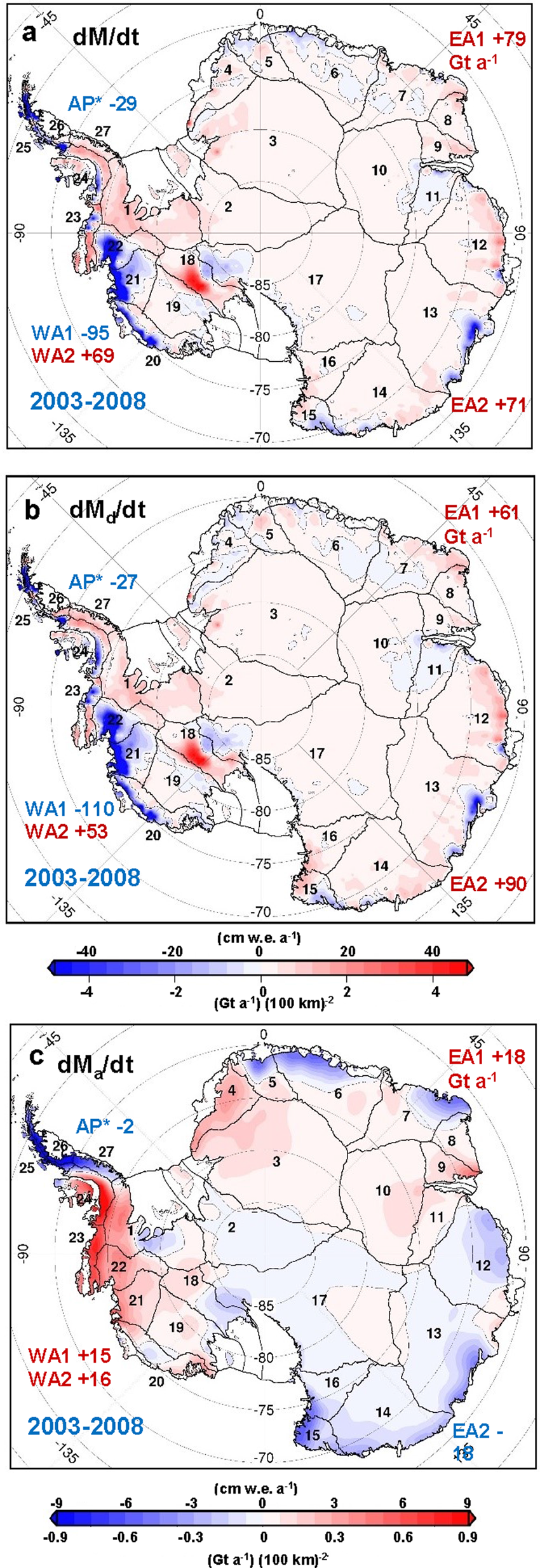
Fig. 16. ICESat maps for 2003–2008, (a) dM/dt, (b) dM d/dt and (c) dMa/dt using dB/dt equal to IvinsdB/dt + δB adj. Rates are linear terms of LQS fits at year 2006.0. *Rates for AP from average-linear-change analysis.

Fig. 17. Maps of the calculated firn density ρ a = ΔM a/Δ(H a−C A) (see text following Eqn (16)) associated with the accumulation driven dM a/dt mass changes for (a) 1992–2001 and (b) 2003–08, showing the large spatial and temporal variations.
7. Antarctic regional changes 1992–2016
The regional changes during 1992 through 2016 are examined for four periods as labeled in Table 7a: (1) the first is the 1992–2001 period of ERS1/2 measurements, (2) the second is the 2003–08 period of ICESat and GRACE measurements and mass-change matching, (3) the third is the 2009–11 period of GRACE measurements, and (4) the fourth is the 2012–16 period of GRACE measurements. The second, third and fourth periods are chosen for the analysis of the linear trends in the ICESat and GRACE M(t) series, because (a) the 2003–08 period has near linear trends and is used for ICESat GRACE mass change matching and (b) there are discernable changes in the slopes of the M(t) series around 2009.0 and around 2012.0 in both the EA and WA regions as well as their sub-regions.
Table 7a. Summary of linear rates of mass change (dM/dt) from ERS1/2, ICESat and GRACE for select periods during 1992–2016

a AP ICESat and all ERS from average-linear-change analysis (Zwally and others, Reference Zwally2015) with ERS using adjusted dB cor from Table 3.
The linear mass trends from LQS fits at the midpoints of the 2003–08, 2009–11 and 2012–2016 periods are in Table 7a and discussed in the next section. The ERS1/2 dM/dt for 1992–2001 are from Zwally and others (Reference Zwally2015) with the (dB cor)2015 in Table 2 replaced with the dB cor in Table 3. The differences between successive periods are given as the deltas in Table 7b along with a comparison of the deltas as fractions of the average-annual SMB. The ICESat and ERS1/2 estimates of uncertainties are made using the methods detailed in the Appendix of Zwally and others (Reference Zwally2015) and for GRACE in Luthcke and others (Reference Luthcke2013).
Table 7b. Summary of changes (delta) in the linear rates of mass change between periods compared to the annual SMB

a SMB from Giovinetto and Zwally (Reference Giovinetto and Zwally2000) and by drainage systems and regions in Zwally and others (Reference Zwally2015).
b These delta are adjusted by 11 Gt a−1 to account for the difference between the 11 Gt a−1 larger ICESat dM/dt from the prior average-linear-change analysis (see Table 2) as was also used for ERS1/2.
In the EA1 sub-region, the rate of mass gain more than doubled from 79 Gt a−1 during 2003–08 to 196 Gt a−1 beginning around the 2009.0. That increased gain of 117 Gt a−1 occurred mostly in the Queen Maud Land portion of EA1, where Shepherd and others (Reference Shepherd2012) and Medley and others (Reference Medley2017) reported mass gains and accumulation increases, but it did not persist after 2012 when the EA1 gain reduced to 88 Gt a−1, close to the prior rate of 79 Gt a−1. In the EA2 sub-region, successive decreases of 10 and 16 Gt a−1 helped to reduce the overall gain in EA from a high of 257 Gt a−1 during 2009–11 to 134 G a−1 during 2012–16, which is similar to the prior rates of 150 Gt a−1 during 2003–08 and 161 Gt a−1 during 1992–2001.
As the mass gain doubled in EA, the mass loss in the coastal WA1 doubled from 95 Gt a−1 during 2003–08 to 214 Gt a−1 during 2009–11. WA1 includes DS22 with the Pine Island Glacier, DS21 with the Thwaites and Smith Glaciers, and DS20 with grounded ice discharging into Getz ice shelf along the coast of Marie Byrd Land. The increased loss of 119 Gt a−1 in WA1 was enhanced by a 39 Gt a−1 reduction in the mass gain in the mostly inland WA2 bringing the total WA loss rate to 187 Gt a−1 during 2009–11. In the last period, the loss from WA1 reduced by 49 Gt a−1 as the gain in WA2 increased by 22 Gt a−1, which together reduced the overall loss from WA to 116 Gt a−1 during 2012–16. This reduced loss is still significantly greater than the 8 Gt a−1 loss rates during 1992–2001 and 29–26 Gt a−1 during 2003–08 from ICESat and GRACE. In the Antarctic Peninsula, the rate of loss increased from 9 Gt a−1 during 1992–2001, to 29–24 Gt a−1 from ICESat and GRACE during 2003–08, followed by losses of 36 Gt a−1 during 2009–11 and 30 Gt a−1 during 2012–16.
The spatial distributions of the rates of dynamic-driven mass changes (dM d/dt), the accumulation-driven changes (dM a/dt) and the total mass changes (dM/dt) during 2003–08 are shown in Figures 16a–c (and S2a, S2b and S2c). The magnitude and spatial distribution of the dM/dt and dM d/dt are very similar and differ from the dM a/dt that are generally smaller and more spatially variable. Areas of significant dynamic thinning are mostly in the coastal areas of WA1, parts of the AP and on the Totten Glacier at 115°E in DS13 of EA2. In DS22 of WA1 with the Pine Island outlet glacier, the dynamic thinning and negative dM/dt both extend inland close to the ice divide except for an area of positive rates in the Southeast corner. Similarly in DS21, dynamic thinning and negative dM/dt extend inland to the ice divide, except for an area of small positive rates in the Southwest corner (see Figs S2a and S2b). Inland dynamic thinning is also inland of the Mercer and Whillans Ice Streams in the Eastern part of DS17 of EA2 and the Western part of DS18 in WA2 inland of the Ross Ice Shelf.
As shown in Figure 16b (and S2), dynamic thickening (discussed further in the next section) extends over most of EA, WA2 and DS27 in the AP. A marked area of dynamic thickening is in DS18 of WA2, inland from the Kamb Ice Stream that stagnated 150 years ago (Joughin and others, Reference Joughin, Tulaczyk, Bindschadler and Price2002), and has a gain of 29 Gt a−1 for 2003–08 adjusted for the new bedrock motion.
8. Discussion and conclusions
During 1992–2016, the AIS changed from a positive mass balance of over 100 Gt a−1, which was reducing sea-level rise by 0.3 mm a−1, to a state of balance close to zero by 2014. The mass balance successively changed from a gain of 144 ± 61 Gt a−1 during 1992–2001, to 95 ± 26 Gt a−1 during 2003–08, to 34 ± 85 Gt a−1 during 2009–11 and to −12 ± 64 Gt a−1 during 2012–2016 (Table 7a). These rates of change suggest an acceleration of −50 Gt a−1 decade−1 during 1992 through 2006, −138 Gt a−1 decade−1 during 2006 through 2010.5, and −105 Gt a−1 decade−1 during 2014.5 through 2016. The changes during 2003–2016, shown in Figures 12 and 13, are driven by the acceleration of outlet glaciers in the coastal WA1 with the marked increase in the dynamic loss of 119 Gt a−1 beginning near the end of 2008 that reduced by 49 Gt a−1 after 2012. The increased dynamic loss near the end of 2008 was enhanced by a 39 Gt a−1 decrease in the gain in WA2 that was followed by an increase of 22 Gt a−1 near the beginning of 2012 driven by accumulation variations. During the same periods, the mass gain in EA increased by 107 Gt a−1 near the end of 2008 followed by a decrease of 124 Gt a−1 after 2012 for a small net gain decrease of 16 Gt a−1 during 2003–2016, also driven by contemporary accumulation variations.
Although the acceleration rates reported by Rignot and others (Reference Rignot2019) of −48 Gt a−1 decade−1 during 1979–2001 and −134 Gt a−1 decade−1 during 2001–2017 are consistent with our acceleration estimates above, the mass-balance results from their input–output method are generally more negative throughout their analysis periods. Although their methods of interpolation or extrapolation for areas with unobserved output velocities have an insufficient description for the evaluation of associated errors, such errors in previous results (Rignot and others, Reference Rignot2008) caused large overestimates of the mass losses as detailed in Zwally and Giovinetto (Reference Zwally and Giovinetto2011).
For all of EA, our mass gains (Table 7a) are essentially unchanged at 161 ± 50 Gt a−1 during 1992–2001, 150 ± 28 Gt a−1 during 2003–08, 257 ± 76 Gt a−1 during 2009–11 and 134 ± 58 Gt a−1 during 2012–2016. The 107 Gt a−1 increase during 2009–11 was driven mostly by a temporary accumulation increase in EA1. The results of Smith and others (Reference Smith2020) for EA, as derived from ICESat to ICESat-2 crossover differences centered, respectively, on 2006.3 and 2019.0, are a gain of 115 ± 21 Gt a−1 (after adding 25 Gt a−1 for the δB adj−Iv of −2.70 mm a−1 as applied to our EA results). The estimated average of our results for the same period (extrapolating the gain of 134 Gt a−1 during 2012–2016 through to 2019.14) is 164 ± 55 Gt a−1 in agreement with Smith within the overlapping uncertainties. In marked contrast, the IMBIE Team (2018) values for EA are much smaller during both 2007–12 at 48 ± 38 Gt a−1 and 2012–17 at −3 ± 30 Gt a−1 (both adjusted by +25 Gt a−1) as they were during 1992–2007.
For all of WA, our mass losses (Table 7a) increased from −8 ± 20 Gt a−1 during 1992–2001, to −28 ± 15 Gt a−1 during 2003–2008, to −187 ± 23 Gt a−1 during 2009–11, to −116 ± 24 Gt a−1 during 2012–16. In coastal WA1, successively-increasing losses of −59 ± 12, −95 ± 9, −214 ± 18 and −165 ± 15 Gt a−1 were partially offset by persistent gains in inland WA2 of 51 ± 14, 68 ± 9, 27 ± 15 and 49 ± 19 Gt a−1. Compared to the IMBIE Team (2018), our losses for WA prior to 2009.0 are ~30 Gt a−1 less negative (after adding 10.53 Gt a−1 to IMBIE for the δB adj−Iv of −6.16 mm a−1 as is applied to our WA results). After 2009.0, our results for WA of −187 ± 23 Gt a−1 during 2009–11 and −116 ± 24 Gt a−1 during 2012–2016 are comparable to both the IMBIE (2018) results of −137 ± 27 Gt a−1 during 2007–2012 and −148 ± 26 Gt a−1 during 2012–2017 (adjusted by 10.53 Gt a−1) and the Smith and others (Reference Smith2020) results of −158 ± 10 Gt a−1 during 2006.3–2019.0 (adjusted by 10.53 Gt a−1).
Also of interest are the 16-year mass changes in the Antarctic ice shelves from Table 1 in Smith and others (Reference Smith2020) showing a loss of 76 ± 49 Gt a−1 from WA and 14 Gt ± 28 Gt a−1 from AP while shelves in EA gained 106 ± 29 Gt a−1. Similarly, during 1992–2002, the ice shelves in WA lost 57 and 38 Gt a−1 in the AP, while shelves in EA gained 142 Gt a−1 as obtained from ERS radar altimetry corrected for radar penetration and temperature-dependent firn compaction (Zwally and others, Reference Zwally2005). Although these inter-decadal changes are small (−20 Gt a−1 in WA, +24 Gt a−1 in AP, −36 Gt a−1 in EA and −32 Gt a−1 overall), they are consistent with significant changes in some drainage systems. The small changes also add support to the validity of our ERS ice-sheet results, because the same altimetry methods were used over both grounded and floating ice during each of the 1992–2001 and 2003–19 periods. Furthermore, the small magnitude of the changes suggests the lack of major inter-decadal ice-shelf thinning or thickening in Antarctica.
Significant regional mass-change rates over Antarctica ranging from tens of Gt a−1 to over 100 Gt a−1 occurred during 1992–2016 as shown by the deltas in Table 7b, including both regional increases in the rates of mass loss and increases in the rates of mass gain. Over all of Antarctica, the total inter-period changes are all increases in mass loss ranging from 40 to 60 Gt a−1, because some regional increases in mass gains only partially or temporarily offset regional increases in losses. Over the 24 years (1992–2016), the total increase in loss is 109 Gt a−1 bringing the total AIS essentially into balance at −12 ± 64 Gt a−1 by 2014. As listed in Table 7b, the ratios of the changes (deltas) to the SMB provide information on the relative significance of the inter-period variations.
In both WA1 and AP, the dynamic-driven variations are more persistent and sometimes larger relative to the SMB than the sub-decadal accumulation-driven variability. In the first interval (between 1992–2001 and 2003–08), when the inter-period change in WA1 was smallest at −36 Gt a−1 (−16% of SMB), the mass loss rate from DS22 with Pine Island Glacier doubled from 12 to 29 Gt a−1 while the loss rate from DS21 with the Thwaites and Smith Glaciers increased from 40 to 51 Gt a−1 and the loss rate from DS20 with glacier flow into the Getz Ice Shelf increased from 7 to 16 Gt a−1 (Zwally and others, Reference Zwally2015). Studies of increases in glacier thinning and acceleration of discharge velocities on Pine Island and Thwaites glaciers in WA1 during ~1992 to the early 2000s include Rignot and others (Reference Rignot, Vaughan, Schmeltz, Dupont and MacAyeal2002), Thomas and others (Reference Thomas2004) and Wingham and others (Reference Wingham, Wallis and Shepherd2009). In the second interval (2003–08 to 2009–11), the loss rate from WA1 further increased by 119 Gt a−1 (−54% of SMB), likely due to continued acceleration of glacier discharge. In contrast, in the third interval (2009–11 to 2012–16.5), the loss rate from WA1 decreased by 49 Gt a−1 (+22% of SMB), likely due to an unidentified slowing of glacier discharge. In the AP, the 20 Gt a−1 (−10% of SMB) loss-rate increase in the first interval (1992–2001 to 2003–08) was related to the acceleration of glaciers, mainly following the collapse of the Larsen B ice shelf (Pritchard and Vaughan, Reference Pritchard and Vaughan2007; Rott and others, Reference Rott, Müller, Nagler and Floricioiu2011; Shuman and others, Reference Shuman, Berthier and Scambos2011). That was followed by a smaller loss-rate increase of 11 Gt a−1 (−6% of SMB) between 2003–2008 and 2009–2011, which was followed by a loss-rate decrease of 6 Gt a−1 (+3% of SMB) between 2009–2011 and 2012–2016.
In EA, and the EA1 and EA2 sub-regions, the inter-period variations of delta/SMB(%) (Table 7b) are mostly only a few percent, which are typical of short-term atmospheric-driven variations in accumulation rates. A marked exception is the aforementioned 117 Gt a−1 increase (+25% of SMB) in EA1 between 2003–08 and 2009–11, followed by a 108 Gt a−1 decrease (−23% of SMB) between 2009–11 and 2012–16. However, the net change in EA1 is only a small increase of 9 Gt a−1 (+2% of SMB) during the ICESat to ICESat-2 period of 16 years. In EA2 during the same times, the rate of mass gain decreased by 10 Gt a−1 (−1% of SMB) between 2003–08 and 2009–11, followed by a 16 Gt a−1 decrease (−2% of SMB) between 2009–11 and 2012–16 giving a net decrease of 26 Gt a−1 (−4% of SMB) during the ICESat to ICESat-2 interval. Therefore, the total accumulation-driven effect for all of EA was a decrease in the rate of 17 Gt a−1 (−1.5% of SMB) from 2003 to 2016, which is most likely not the cause of the mass gain of 90 Gt a−1 in EA during the ICESat to ICESat-2 interval that was reported by Smith and others (Reference Smith2020).
Furthermore in EA during both of the earlier periods (1992–2001 and 2003–08), there were small negative accumulation anomalies of −11.6 ± 6 Gt a−1 (i.e. −1% of SMB) compared to the 27-year mean from 1982, which justified our conclusion that the mass gain in EA in those periods was dynamic ice thickening and not due to increases in contemporaneous snowfall (Zwally and others, Reference Zwally2015). In the last column of Table 7b, we show the net changes in the rates over the 25 years (1992–2016) by including the rates of mass change during the first interval (i.e. between 1992–2001 ERS and 2003–08 ICESat). These inter-decadal changes are very small at −17 Gt a−1 (−1% of SMB) for EA, −2 Gt a−1 (0% of SMB) for EA1 and −15 Gt a−1 (−2% of SMB) for EA2, further supporting our conclusion that the observed mass gains in EA are from on-going dynamic thickening and not from current trends in accumulation.
The observed dynamic thickening (2003–08) extends over most of EA (Figs 16b and S1) and much of the inland WA2, as was also shown for 1992–2001 in Figure 11a of Zwally and others (Reference Zwally2015). The average dynamic thickening from the 2003–08 ICESat analysis is 16.4 mm a−1 over EA and 47.7 mm a−1 over WA2 (Table 3). Comparable thickening rates were previously obtained from the average-linear-change analysis (Zwally and others, Reference Zwally2015), which were 17.5 mm a−1 for 1992–2001 and 18.6 mm a−1 for 2003–08 over EA, and 55.0 mm a−1 for 1992–2001 and 62.1 mm a−1 for 2003–08 over WA, after respective adjustments of δB adj−Iv = −2.7 mm a−1 for EA and −6.2 mm a−1 for WA (Table 4).
Ice dynamic changes are driven by long-term changes in accumulation, but those dynamic changes remain small for long periods of time (e.g. 100–10 000 a) as changes in accumulation slowly change the ice thickness, which in turn slowly changes the gravitational forcing of the ice velocity. For decadal and sub-decadal changes that are driven by atmospheric variations in accumulation, the corresponding dynamic response is very small, including for the relatively large +25% and −23% of SMB variations in EA discussed above. Therefore, our conclusions of dynamic ice thickening in both EA and WA2 during 1992–2016 are based on the absence of persistent accumulation-driven mass changes during that time period.
However, over much longer times (e.g. >1000 a), a sustained change in accumulation significantly alters the ice velocity so that any conclusions on long-term dynamic thickening (or thinning) necessarily depend on other evidence of long-term changes. An example is the marked increase in accumulation that began in the early Holocene (~10 ka BP), with a 67–266% increase after the LGM as derived from the Vostok ice core and radar-layer linking to four other locations (Siegert, Reference Siegert2003). During the preceding 100 ka, accumulation had diminished from ~15–12 mm w.e. a−1 as the climate cooled during the Glacial Period giving the EA ice sheet a long time to reach a dynamic balance with the low accumulation rate. During the Holocene as shown in Figure 2 of Siegert (Reference Siegert2003), the accumulation at Vostok Station was sustained at a higher level of 22 mm w.e. a−1 after rising from 12 mm w.e. a−1 following the LGM. That sustained larger accumulation rate and consequent slow acceleration of the ice flow was the basis for the conclusion of long-term dynamic thickening in EA made in Zwally and others, Reference Zwally2015. As noted in the introduction, ice growth in EA also indicated Holocene glacier advances from the EA ice sheet through the Transantarctic mountains into the Dry Valleys (Stuiver and others, Reference Stuiver, Denton, Hughes and Fastook1981; Denton and Wilson, Reference Denton and Wilson1982).
The effect of a long-term sustained increase in accumulation on ice thickening, and consequently the ice velocity in a large ice sheet is shown by the following basic consideration in Zwally and others (Reference Zwally2015): a 20 mm a−1 elevation increase in central EA causes only a 200 m elevation increase over 10 000 years, producing a correspondingly small ~6% increase in the driving stress under 3400 m of ice and therefore a very slow acceleration of the ice flow increasing slowly with time. In addition, a 3-D numerical model (Wang and others, Reference Wang, Li and Zwally2012) of the dynamic response of the ice flow in central EA (e.g. near the ice divide in DS13 ~105°E) to a doubling of accumulation after the LGM showed the surface elevation of the grounded ice increasing at a nearly constant rate of 20 mm a−1 for 10 ka, reaching a 200 m elevation increase at present, followed by a future decreasing rate of rise continuing asymptotically to a total 320 m elevation increase in another 30 ka (Wang and others, Reference Wang, Li and Zwally2013).
Similar to EA, the present accumulation rate in WA at present is around twice that of the ice age rate 6400–16 000 years ago (Siegert and Payne, Reference Siegert and Payne2004). However, as noted in the introduction, the long-term dynamic ice history of WA with a major retreat after the LGM followed by a Holocene readvance (Bradley and others, Reference Bradley, Hindmarsh, Whitehouse, Bentley and King2015; Kingslake and others, Reference Kingslake2018) is very different from the very long-term dynamic stability of EA. For the inland WA2, our finding of −3.48 mm a−1 subsidence (δB 0−avg) is in contrast to the average uplifts ranging from 3.00 to 5.42 mm a−1 from the three GIA models. As discussed in Section 6, the reasons for the difference are: (1) the differing ice-loading history in WA2 associated with the post-2014 findings of a Holocene readvance of the grounding lines of the Ross and Filchner-Ronne Ice Shelves from their maximum post-LGM inland retreats, which is not in the history of the earlier GIA models, and (2) the findings of Barletta and others (Reference Barletta2018) of a lower mantle viscosity in WA and the consequent significantly-faster GIA response times compared to those of the higher-viscosity GIA models.
A primary glacial forcing for GIA models in WA is from the loss of ice associated with the post-LGM thinning of the ice sheet, shown in one reconstruction (Bentley and others, Reference Bentley2014) as a decreasing elevation at a location near the ice divide in WA2 from 200 m above the present level at 20 ka BP to the present elevation at a rate of 50 m every 5 ka. That post-LGM ice loss was a principal driver of the Antarctic contribution to global mean sea-level rise that started rising ~15 ka BP and was mostly complete by ~9 ka BP (Pollard and others, Reference Pollard, Gomez and DeConto2017).
Specific evidence for a different ice-loading history in WA2 after ~10 ka BP includes a 400 km Holocene readvance of the grounding line of the Ross Shelf from its inland retreat at 9.7 ka BP and a smaller readvance of the Filchner-Ronne Ice Shelf from its retreat at 10.2 ka BP (Kingslake and others, Reference Kingslake2018) with associated low post-glacial rebound rates in the Weddell Sea (Bradley and others, Reference Bradley, Hindmarsh, Whitehouse, Bentley and King2015). Similar retreats and readvances are also shown (personal communication from David Pollard, 2020) in climate-driven ice-sheet modeling such as Pollard and others (Reference Pollard, Gomez and DeConto2017). In Section 6, we discussed evidence for ice thickening of several hundred meters over a large area of the lower portions of DS18 and 19 during the mid-to-late Holocene causing an increase in the ice loading of several hundred meters over a rather large area of DS18 and 19 in WA2. We also noted that thickening of the lower portions can also restrain the ice flow and lead to inland thickening as is occurring in DS18 as shown in Figure 9b (and S1b). The 2003–08 mass gain in DS18 is 29 Gt a–1 (adjusted from the 27.3 Gt a–1 in Zwally and others, Reference Zwally2015).
As noted in Section 3, the response times can range from decadal to centennial for the lower viscosities found in WA1, the Antarctic Peninsula, Patagonia and elsewhere to the millennial responses for the higher viscosities used in Antarctic GIA models. In Section 6, we estimated that for the millennial response times of the high viscosity models with ~5 response times since the beginning of the Holocene 10 ka BP, the exponentially decaying uplift from post-LGM ice unloading would be reduced by a factor of ~7 × 10⁻³. In contrast, for the lower-viscosity decadal-to-centennial response times, the corresponding reductions would be by a much-larger factor of <~2 × 10⁻²². Therefore, the primary on-going response should be subsidence from the later Holocene readvance that has been driven by the associated thickening of the grounded ice sheet. Subsidence is also consistent with our currently observed dynamic thickening in WA2.
We note again that our procedures for adjustment of the GIAcor and dB cor are based on the simple principle that the respective corrections are caused by the mass and volume changes of the same material in the Earth's mantle underlying the ice sheet. The matching is based on a simple linear relationship between the uncorrected GRACE and ICESat mass changes using a constant determined by the ratio of the mass change to the volume change. Although we find that the values of RatioG/dB from the GIA models give values of ρ earth that are consistent with the knowledge of mantle densities, that physical correspondence is not essential for making the δB adjustments. However, we believe that the physical relationship implied by the consistency of the ρ earth values strengthens the validity of our adjustments to the ICESat and GRACE mass estimates.
Finally despite the quality of GIA models, their results are very dependent on model parameters such as mantle viscosity that are estimated using model constraints from limited measurements of sea-level change and crustal motions, which are not measurable in vast ice-covered areas of Antarctica. Furthermore, the GIA models have been highly dependent on ice-sheet models and glacial-geologic evidence for their ice-loading histories that force the mantle flow. We believe our results on Antarctic dynamic thickening and our derived adjustments provide useful information that can be used for further development of the GIA models along with the recent new information on the ice loading history. Also, our attempts to calculate the spatial distribution of RatioG/dB and therefore calculate the spatial distributions of the bedrock motion adjustments for ICESat and GRACE dM/dt matching (rather than regional averages) were limited by the singularities at small values and perhaps the numerical precision of the GIA model results. Therefore, the examination of the RatioG/dB within the models, its spatial distribution and its implications regarding the density of the fluid mantle involved may provide new insights and perhaps methods for avoiding the numerical problems we encountered using the current GIA and dB/dt outputs to calculate their ratio.
Although the inter-decadal changes in total Antarctic accumulation since 1992 have been very small, future increases in accumulation with climate warming are likely to have an increasing impact on the overall Antarctic mass balance. A 200-year reconstruction of Antarctic snow accumulation (Medley and Thomas, Reference Medley and Thomas2019) showed that increased accumulation mitigated 20th-century sea-level rise by ~10 mm since 1901 at an average rate of 0.11 mm a−1 (40 Gt a−1) from 1901 to 2000 and a higher rate of 0.25 mm a−1 (88 Gt a−1) from 1979 to 2000, which is consistent with our mass gain of 144 ± 61 Gt a−1 from ERS1/2 during 1992–2001. In that regard, the EA ice sheet is especially important because of its large area contributing 73% of the aforementioned 20th-century mass gain and sea-level rise mitigation. Estimated sensitivities of the total Antarctic mass balance to temperature change range from −0.36 to −0.80 mm a−1 of global sea-level change per °C (equivalent to +130 to +290 Gt a−1 of ice per °C) (Huybrechts, Reference Huybrechts, Bamber and Payne2004 in Bamber and Payne, Reference Bamber and Payne2004). The largest estimate of −0.80 mm a−1 sea-level change per °C includes the interactive effect on accumulation from changes in sea ice extent by 125 km per °C (i.e. distance to open-ocean source of moisture) from Giovinetto and Zwally (Reference Giovinetto and Zwally1996). A smaller estimate of −0.27 mm a−1 per °C change in SMB is from a regional atmospheric climate model forced by the future climate of a global climate model (Ligtenberg and others, Reference Ligtenberg, van de Berg, van den Broeke, Rae and van Meijgaard2013). We also calculate −0.28 mm a−1 per °C change from the temperature and precipitation data for 60° to 90°S as used in Golledge and others (Reference Golledge2019) for several RCP climate prediction scenarios. Such accumulation-driven increases, along with the current long-term dynamic thickening in EA and WA2, might continue to offset some increases in dynamic losses such as those that have occurred in the AP and the coastal WA1.
However, the decadal-scale dynamic changes are not all causing increases in mass loss. The M(t) for the AP in Figure 14 shows reduced mass loss for the last several years. Also, as previously noted, the M(t) for WA1 in Figure 13 shows that the marked increase in dynamic loss that began around 2009 reduced some during the later years, possibly related to the solid Earth and sea-level feedbacks modeled by Larour and others (Reference Larour2019). Interestingly, the Kingslake model simulation does not show a post-LGM retreat to inside the present grounding line in the Amundsen Sea sector of WA1, which may have implications regarding the ongoing changes and the possible limited extent of future ice losses in WA1. Also, Barletta and others (Reference Barletta2018) note that their finding of a lower mantle viscosity and shortening of the response time to mass changes to ‘decades up to a century … increases the potential stability of the WAIS against catastrophic collapse’, with implications for the stability of the inland WA2 as well .
Table 8. ICESat laser campaign biases determined over leads and polynyas in sea ice

DSL are the ICESat measured D corrected for changes in SSH measured concurrently by Envisat.
Table 9. Accumulation density (ρ a) and pseudo density (ρ pseudoI) by region

ρ a is density associated with δA(t) anomalies.
ρ pseudoI = dM/dt/dI/dt.
Figures S1 and S2 in alternate multi-color scales to Figures 9 and 16, as previously used in Zwally and others (Reference Zwally2015) for example, are included in the Supplementary Material along with a link to the digital data used in those figures.
Supplementary material
The supplementary material for this article can be found at https://doi.org/10.1017/jog.2021.8.
Acknowledgements
We appreciate the GIA and dB/dt model data provided by E. Ivins, P. Whitehouse and R. Peltier. NASA GSFC mascon solutions were developed partly under the NASA GRACE and GRACE Follow-On Science Team Grant NNH15ZDA0-01N. This research was also supported by NASA's ICESat project science funding. We appreciate the reviewers' efforts and their helpful comments, especially those of the fourth reviewer with expertise in GIA processes and an anonymous colleague for thorough reading of the manuscript and helpful suggestions. Following our original submission, the Editors' requested addressing reviewers' concerns about why our ICESat results on Antarctic mass gains differ from others in the literature. That request resulted in additional documentation of the validity of our ICESat and ERS1/2 results and our methodologies and reasons why we believe the results of others had some significant errors, now in Section 5 and the Appendix. It also led to the inclusion of the supportive Envisat results and co-author F. Rémy. We also greatly appreciate the dedicated efforts of so many scientists, engineers, analysts, and managers in NASA and supporting companies that led to the successes of the ICESat missions and similarly of the many individuals involved in the successes of GRACE and the ESA missions of ERS and Envisat.
Appendix
Introduction
We examine the compatibility of elevation changes derived from satellite altimeters including basic corrections made to the data, the methods to obtain valid ice-sheet elevation changes, and the methods to derive mass changes from the elevation changes. We review our methods and provide reasons why our results differ from some studies and agree with others. The first type of reason includes differences in the various corrections and calibrations applied in the data processing and those that may be developed later by investigators. For radar altimetry, a second reason is differences in the methods of correcting for the highly-variable penetration of the radar signal into the firn and the depth of the backscatter signal detected by the altimeter, from which the range to the surface is derived, thereby affecting the derived H(t) and dH(t)/dt. The third reason is differences in the methods of deriving mass changes from the measured elevation changes, which includes (1) accounting for the densities of the firn and ice that are associated with the elevation changes, (2) corrections for firn compaction (FC), and (3) correction for the dB/dt bedrock motion, thereby affecting the M(t) and dM(t)/dt.
Basic corrections and elevation-change analysis
An example of the first reason from Zwally and others (Reference Zwally2005) is: ‘Instrument corrections include subtraction of a 40.9 cm bias from ERS-1 elevations to account for a different instrument parameter used for ERS-2 (Femenias, Reference Femenias1996) and corrections for drifts in the ultra-stable oscillator and bias changes in the scanning point target response that are obtained from the European Space Agency’. Those corrections required application by the data users and are not necessarily applied nor noted in publications. A second example is the correction for the ERS-1/ERS-2 inter-satellite elevation bias that was discovered and empirically-determined during 13 months of simultaneous operation; from Zwally and others (Reference Zwally2005): ‘The bias correction lowers the ERS-2 elevations by an average of … 17.5 cm … over Antarctic grounded ice and by 12.0 cm… over Antarctic floating ice. … the correction lowers the average dH/dt by 2.4 cm a−1… on grounded ice and by 1.6 cm a−1… on floating ice. The effects … on calculations of mass change (dM/dt) for the ERS gridpoints are roughly … –205 Gt a−1 for Antarctica … indicating the importance of this correction. Davis and others (Reference Davis, Li, McConnell, Frey and Hanna2005) in effect apply a bias correction by calculating separate H(t) series for ERS-1 and ERS-2 and adjusting them together during the 12 month overlap period, but do not state the magnitude of their adjustments’. This elevation bias was very spatially variable over the ice sheet and at least partially related to the surface slope.
Another important factor is our use of ERS ice-mode data only, because we found that ocean-mode only and mixed-mode data had differing biases that were also spatially variable and difficult to determine. Davis and others (Reference Davis, Li, McConnell, Frey and Hanna2005) also used ice-mode data only that were obtained with corrections from our reprocessing of ESA provided data. At this level, it is possible to inter-compare results from some studies, but not all.
Another factor affecting the accuracy of the derived elevation changes is the methods used for crossover analysis and construction of elevation time series from which dH/dt is derived. Our methodology (Zwally and Brenner, Reference Zwally, Brenner, Fu and Cazanave2001; Zwally and others, Reference Zwally2005) includes two important features that affect the accuracy: (1) the averaging of elevation differences at ascending–descending crossovers with those at descending–ascending crossover differences according to Eqn (20) in Zwally and Brenner (Reference Zwally, Brenner, Fu and Cazanave2001) [a method first used in Zwally and others (Reference Zwally, Brenner, Major, Bindschadler and Marsh1989) to remove orbital biases but also removes the effects of penetration (Arthern and others, Reference Arthern, Wingham and Ridout2001)], and (2) the construction of time-series from crossover differences that uses not only crossovers between the first repeat cycle and all successive repeat cycles, which gives N terms for N repeat cycles including N pairings of crossover differences (e.g. Wingham and others, Reference Wingham, Ridout, Scharroo, Arthern and Shum1998), but also uses crossovers between the second repeat cycle and all successive cycles, plus between the third repeat and all successive repeats, and so forth constructing a series also with N terms but includes N 2/2 pairings of independent crossover differences. The quality of the time series in select 50 km squares from which the dH/dt are calculated was shown in Figures 3 and 4 in Zwally and others (Reference Zwally2005).
ICESat inter-campaign biases and G-C error correction
As described in Zwally and others (Reference Zwally2015): ‘We use methods … used in … mapping of the level of open water and thin ice in leads and polynyas in sea ice by ICESat in the Antarctic (Zwally and others, Reference Zwally, Yi, Kwok and Zhao2008) and the Arctic (Farrell and others, Reference Farrell, Laxon, McAdoo, Yi and Zwally2009), in the joint mapping by ICESat and Envisat of the mean dynamic topography in the Arctic Ocean (Farrell and others, Reference Farrell2012), and in the analysis of temporal changes in the ocean dynamic topography … by Envisat in the western Arctic Ocean (Giles and others, Reference Giles, Laxon, Ridout, Wingham and Bacon2012). Advantages of our method compared to other studies of campaign biases … include: (1) smooth surfaces in leads and polynyas that do not require a sea-state bias … correction, (2) measured laser reflectivity of 0.42 that is closer to the 0.53 reflectivity of the adjacent sea ice and of ice sheets compared to the measured low reflectivity of 0.12 over open ocean, (3) availability of independent Envisat measurements of the vertical motion of the sea surface reference level, and (4) coverage over the reference surface by most of the laser tracks during each campaign.’
‘As of December 2012, the ranges for ICESat/GLAS … ice-sheet data products had been incorrectly calculated from the centroid (amplitude-weighted center of leading and trailing edge thresholds) of the transmit laser pulse to the center of a Gaussian fit of the return pulse (Zwally, Reference Zwally2013). Applying the range correction for the transmit Gaussian to centroid (G-C) offset improved the range precision by 1.7 to <2 cm, and changed (but did not remove) the laser campaign biases (Zwally, Reference Zwally2013). Our current analysis uses elevation data with the G-C correction applied and compatible bias corrections determined with data with the G-C correction also applied. Before the G-C correction was applied, the G-C offset had been in both the data for the ice-sheet dh/dt along-track solutions and in our bias calculations, so the effect of the offsets cancelled. We confirmed that cancellation by comparing our previous and current analyses of dH/dt. The average dH/dt for the AIS changed by only +0.01 cm a−1, and the average dH/dt error reduced from 0.024 to 0.012 cm a−1, reflecting the improved range accuracy. The corresponding dM/dt for the AIS changed by only +1 Gt a−1. Therefore, although the net effect of using ice-sheet data without the G-C correction applied is very small if commensurate bias corrections are applied, the error is significant (−1.29 cm a−1) if the G-C correction is only applied to the data and not to the bias determinations (i.e. incorrectly causing a less positive or more negative dH/dt). The error is similar if the G-C correction is applied, but … [earlier, before G-C corrected)] bias adjustments are applied as in Helm and others (Reference Helm, Humbert and Miller2014) in which the volume change obtained from ICESat for 2003–09 for the AIS is [consequently too] negative at –60 ± 44 km3 a−1.’ Helm and others (Reference Helm, Humbert and Miller2014) value of −23 ± 36 km3 a−1 (ICESat 2003-09) for EA would adjust to +109 ± 36 km3 a−1 if their laser biases had been estimated using data with the G-C correction applied. Scambos and Shuman (Reference Scambos and Shuman2016) also compared an incompatible mixture of biases estimated using data with or without the G-C correction applied.
Importantly, before the G-C error was discovered, the trend in the estimated biases determined without the G-C correction was small, so that applying those bias corrections improved the relative accuracy of the laser campaigns (https://nsidc.org/data/icesat/laser_op_periods.html) but made only a small change in trends derived from the data. Specifically, using biases determined over open-water and thin ice in the Arctic Ocean from Zwally and others (Reference Zwally2011): ‘We reduce the time variation of these d values [biases] by 0.003 m a−1 to account for the current rate of sea-level rise, and then subtract the reduced d values from the measured elevations. The linear trend in the reduced d is 0.006 m a−1, which averaged over all of Greenland increases the overall mass loss by 9 Gt a−1 compared with data without the d correction applied.’
Shepherd and others (Reference Shepherd2012) IMBIE-1 included mass gain estimates from ICESat for EA (in Table S8) of 118 ± 56 Gt a−1 by Sorensen and Forsberg, 126 ± 60 Gt a−1 by Smith, and a smaller gain of 86 ± 55 Gt a−1 by Yi and Zwally, all of which were done before the G-C laser error correction was discovered, and therefore were done with campaign bias corrections consistently determined. As noted above, trends in the bias corrections were small before the G-C correction, but changed significantly afterward. Shepherd and others (Reference Shepherd2018) IMBIE-2 did not include ICESat results from Forsberg nor Smith and at least some of the included ICESat results from other investigators (other than Zwally) had laser biases determined with the G-C inconsistency causing a significant dH/dt bias as noted on NSIDC ICESat-data website in 2013.
The bias corrections used in this paper in Table 8 are the same as those in Zwally and others (Reference Zwally2015), except for the addition of values for campaigns L2d and L2F in 2009 and the removal of a sinusoidal component with a peak-to-peak amplitude of 4.3 cm and with maxima at day 123 of the annual cycles. These and other bias estimates are available at https://nsidc.org/data/icesat/correction-to-product-surface-elevations.html along with the evaluation criteria such as whether a correction was made for an independently determined vertical motion of the reference surfaces. The NSIDC website includes the recommendation: ‘Applying the per-shot G-C changes, but does not remove all the inter-campaign biases. Any new “campaign level” bias adjustments should be determined with compatible (corrected) data and applied only to analysis of corrected data’.
Variable radar penetration and backscatter depth
Ice-sheet surface elevations measured by radar altimeters are seriously affected by the strengths of the surface reflection and the sub-surface volume scattering and reflection from internal layers, which were modeled and analyzed in altimeter waveform data over Greenland and Antarctica (Partington and others, Reference Partington, Ridley, Rapley and Zwally1989). Numerous other papers also addressed the spatial variability of the penetration and its effects on various waveform retracking algorithms, and therefore on the calculated ‘surface’ elevation. In general, altimeter waveforms as depicted in Figures 4–6 in Partington and others (Reference Partington, Ridley, Rapley and Zwally1989) have an initial rise (return vs time) with a slope that is dependent on surface roughness (on the scale of sastrugi) as the pulse-limited footprint expands over the surface, followed by a decreasing return from the radar penetrating into the firn and the consequent volume scattering and reflection from internal ice layers. The three principal waveform-retracking algorithms differ mainly in their points selected on the waveform for the range correction, and therefore differ in the level of their derived surface or near-surface elevation. The threshold tracker (Davis, Reference Davis1997), which selects a point on the leading edge at 20% of the waveform peak, is least sensitive to sub-surface returns, as is the similar threshold first maximum retracker (TFMRA) (Helms and others, Reference Helm, Humbert and Miller2014). The multi-parameter waveform fitting tracker (Martin and others, Reference Martin, Zwally, Brenner and Bindschadler1983) selects the mid-point of the leading edge corresponding to the mean surface elevation and is also relatively insensitive to volume scattering. In contrast, the Offset-Center-of-Gravity (OCOG) (Bamber, Reference Bamber1994), used by Wingham and others (Reference Wingham, Ridout, Scharroo, Arthern and Shum1998) and by ESA for one of the CryoSat data products, uses the whole waveform and is therefore more sensitive to the sub-surface backscatter and its variability.
While retracking algorithms give different surface or sub-surface elevations, and may have differing accuracies and precisions, those differences would not be a major problem for the measurement of elevation changes if the strengths of the surface reflection and the sub-surface reflections and scattering were constant in time. However, the penetration/reflection depth and the backscatter power are highly-variable seasonally and have multi-year trends, as clearly shown in Figure 3 of Yi and others (Reference Yi, Zwally, Cornejo, Barbieri and DiMarzio2011). Adodo and others (Reference Adodo, Rémy and Picard2018) provide a detailed analysis of the seasonal variations of the backscattering over the Antarctic ice sheet including the theoretical dependence on firn properties and analysis of multi-frequency radar-altimeter measurements made by Envisat and SARAL/AltiKa.
The first elevation correction for the temporal variability of the penetration depth as a function of radar backscatter used the ‘gradient’ of the observed elevation to strength the backscatter derived from the waveforms (note 10 in Wingham and others, Reference Wingham, Ridout, Scharroo, Arthern and Shum1998). The gradient was called ‘sensitivity’ in Zwally and others (Reference Zwally2005), who used the altimeter AGC as a measure of the backscatter and applied other correlation criteria for its application as shown in Figure 6 of Yi and others (Reference Yi, Zwally, Cornejo, Barbieri and DiMarzio2011), thereby improving the correction. Yi and others (Reference Yi, Zwally, Cornejo, Barbieri and DiMarzio2011) also considered alternate methods (short-term, mixed-term and long-term) of calculating the sensitivity that give different sensitivities and correlation coefficients. Successful corrections for ERS1/ERS2 were also made by Davis and Ferguson (Reference Davis and Ferguson2004) and Khvorostovsky (Reference Khvorostovsky2012).
Unfortunately for Envisat and CryoSat data, the correction for the time-variable penetration depth became substantially more difficult. The linearly-polarized radar signals, which were oriented across-track on Envisat at 120° and CryoSat at 90°, interact with firn properties related to the direction of the surface slope (sometimes called surface anisotropy) and the relative directions (polarization vs surface slope) differ significantly at track crossings (e.g. Legresy and others, Reference Legresy, Rémy and Schaeffer1999; Arthern and others, Reference Arthern, Wingham and Ridout2001; Rémy and others, Reference Rémy, Flament, Blarel and Benveniste2012). In contrast, the orientation of the polarization along-track (at 0°) on ERS1/ERS2 tended to be more oriented in the direction of maximum surface slope at high-latitude crossovers rather than across-slope, especially at the steeper ice-sheet margins, which may have enabled the more successful penetration corrections for ERS crossover analysis.
For Envisat data, a successful correction was developed using repeat-track analysis and an advanced correction algorithm (Flament and Rémy, Reference Flament and Rémy2012). Repeat-track analysis significantly mitigates the variable penetration problem, because the polarization orientation relative to the surface slope is essentially identical on the repeating tracks. A critical point is that their solution makes a time-dependent backscatter correction for the variable depth penetration, and also uses time-variable waveform parameters. They used 84 of the 35-day repeat cycles from September 2002 to October 2010 and computed ‘the elevation trend every kilometer along-track’ using ‘All available measurements within a 500 m radius of a point on the mean ground track’. ‘… In the central part of the East Antarctica, the height and the leading edge width fluctuations vary together while elsewhere, height fluctuations may occur with no variations in the waveform shape, mostly during winter. As a consequence, these induced errors cannot be corrected with solely the help of the backscatter: waveform shape parameters are also needed. They are however not enough to fully correct these two errors. We propose an empirical correction for these effects. … In terms of volume change, the estimation may vary up to 4 cm a−1 at cross-overs depending on the correction used and is reduced in average to 2.3 cm a−1 with our correction. The difference between the height trends estimated with both corrections is weak in average but may locally reach 5 cm a−1 with a clear geographical pattern.’
Consistency of the dH/dt from Envisat radar altimetry after correction for the variable-radar penetration is shown in the comparisons in Figures 9, 10 and S1 with the corrected dH/dt from ERS1/ERS2 and the dH/dt from the ICESat laser altimetry. The three average dH/dt over EA from ERS1/ERS2, ICESat and Envisat are 10.7, 13.1 and 8.3 mm a−1 showing agreement at the level of only a few mm a−1.
The method of McMillan and others (Reference McMillan2014) for CryoSat is: ‘To compute changes in … elevation, we adapted a repeat-track method (Smith and others, Reference Smith, Fricker, Joughin and Tulaczyk2009; Moholdt and others, Reference Moholdt, Nuth, Hagen and Kohler2010; Flament and Rémy, Reference Flament and Rémy2012) to suit the Cryosat-2 dataset, …’ and ‘…Elevation measurements are accumulated in 469 451 regularly spaced (5 by 5 km) geographical regions, and within each region, we solve, simultaneously, for spatial and temporal fluctuations in elevation and for a fixed contribution due to the impact of surface anisotropy on the tracked range (see supporting information)…, …and a correction is applied to account for temporal fluctuations in backscatter that cause spurious fluctuations in range (Davis and Ferguson, Reference Davis and Ferguson2004; Khvorostovsky, Reference Khvorostovsky2012; Wingham and others, Reference Wingham, Ridout, Scharroo, Arthern and Shum1998)’. Their solution is complicated because: (1) their 5 km covers a 100× larger area with more variable surface conditions than that used by Flament and Rémy (Reference Flament and Rémy2012) and the long 365-day near-repeat cycle includes few near-repeat orbits, (2) their ‘contribution’ for the ‘impact of surface anisotropy’ is very large (+1 to −1 m in their Supplementary Material Figs 1 and 3); their separation into fixed and time-varying fluctuations is of dubious validity. Their range measurements are ‘corrected for the lag of the leading edge tracker’ (Wingham and others, Reference Wingham, Shepherd, Muir and Marshall2006), which used ERS ‘WAP v. 3 altimeter data’ and presumably the OCOG retracker that is more sensitive to sub-surface penetration.
In contrast, Helm and others (Reference Helm, Humbert and Miller2014) stated: ‘… our study show(s) that a correction for the static “Antarctic pattern” in dh/dt estimates as applied in McMillan and others (Reference McMillan2014) (for penetration) can be avoided when using the TFMRA re-tracker’. Table 4 in Helm and others (Reference Helm, Humbert and Miller2014) for EA shows volume changes of +78 ± 19 km3 a−1 (IMBIE 2003–2008) and +59 ± 63 km3 a−1 (CryoSat 2011–14), compared to the −2.7 ± 33 km3 a−1 (CryoSat 2010–2013) from McMillan and others (Reference McMillan2014), giving a 62 ± 71 km3 a−1 difference between CryoSat investigators for EA.
For Greenland, Nilsson and others (Reference Nilsson, Gardner, Sørensen and Forsberg2016) showed that an improved leading-edge retracker for CryoSat-2, which changes the sensitivity to depth penetration, can cause a very-large 50 cm a−1 difference in the derived surface elevation in the normally dry snow zone of Northern Greenland and significant differences in the volume change estimates compared to ESA's public data product.
Deriving mass changes from elevation changes
Our methods of deriving mass changes, as applied to Greenland (Zwally and others, Reference Zwally2011) and to Antarctica (Zwally and others, Reference Zwally2015) and followed in this paper for the dM/dt, dMd/dt and Ma/dt in Figures 16 and S2, have distinct advantages not employed in other studies. The advantages are: (1) correction for accumulation-driven and temperature-driven changes in surface elevation that do not involve changes in mass using a state-of-art FC model (Li and Zwally, Reference Li and Zwally2015); and (2) separation of accumulation-driven and dynamic-driven mass changes and the assignment of proper ice (ρ i) and near-surface firn (ρ a) densities to each, even though ρ a is not necessarily calculated (see text following Eqn (13)).
Initially, investigators used a single density ρ to estimate dM/dt = ρ × dH/dt (with dH/dt corrected for bedrock motion and perhaps FC), even though it was known that elevation changes were likely due to a combination of accumulation-driven changes with a density of ρ a and dynamic-driven changes with the density of ρ i. For example, Zwally and others (Reference Zwally2005) calculated a mass change dF/dt using ρ a, = 0.4, which ‘is a typical mean density for the top strata corresponding to 10 years of accumulation’, and dM/dt using ρ i = 0.91, which provided their preferred estimate. Clearly, choosing either ρ a or ρ i makes a factor of 2.3 or more difference causing significant errors in mass estimates one way or the other.
More recently, users of the old method (e.g. McMillan and others, Reference McMillan2014; McMillan and others, Reference McMillan2016; Martín-Español and others, Reference Martin-Español, Bamber and Zammit-Mangion2017; Schroder and others, Reference Schroder2019) take dM/dt to be equal to ρ firn/ice × dH/dt, where H is corrected for bedrock motion and perhaps FC, and ρ firn/ice is chosen/assumed to be either ρ firn equal to ~0.350 or ρ ice equal to 0.917, sometimes based on a limited spatial mask as in McMillan and others (Reference McMillan2014) and Schroder and others (Reference Schroder2019). From McMillan and others (Reference McMillan2016): ‘To convert the resulting altimeter rates of change to mass, we constructed a density model that accounted for both surface and dynamic processes. In regions where high rates of elevation change and ice flow suggested a state of dynamic imbalance, we used an ice density of 917 kg m−3 (see Text S8). Elsewhere, detected elevation changes were assumed to be driven by SMB processes, and we used an ice density within the ablation zone and the density of the IMAU-FDM firn layers gained or lost across the remaining areas’, for which use of the density of firn layers instead of their former 350 kg m−3 made a small improvement. However, the method maintains the critical flaw of not actually accounting ‘for both surface and dynamic processes’ where surface and dynamic processes occur in the same location, which is mostly everywhere in the accumulation zone.
As we noted following Eqn (16), ‘a priori selection of appropriate single or multiple firn/ice densities … is not possible due to the extensive spatial and temporal variabilities of the actual ρ a, and because H a and H d have differing spatial variations in magnitude and sign’. This is further illustrated for Greenland in Zwally and others (Reference Zwally2011) in their Figure 7 ‘Maps for the 2003–07 period. (a) Accumulation-driven elevation change, dH aCA/dt. (b) Ablation- and dynamic-driven elevation change, dH bd/dt. (c) Relative density, ρ a, of the firn for the dH aCA/dt component’. Their Figure 7b clearly shows the extensive area of dynamic thickening over much of the higher elevations of the accumulation zone, and in their Figures 7a and b, the mixture of surface and dynamic processes everywhere. The large variability of the density for the surface processes is shown in their Figure 7c. Furthermore, the surface processes (i.e. H aCA(t)) are more variable with time on decadal and sub-decadal time scales, and therefore vary in sign from the more constant dynamic processes, both of which contribute to the measured H(t) according to Eqn (12).
Similarly for Antarctica, the large spatial and temporal variations of the accumulation-driven mass change, dM a/dt, are shown in Zwally and others (Reference Zwally2015) in their Figure 10a for 1992–2001 and 10b for 2003–2008, and are also evident in the measured dH/dt in their Figures 6a and b. In contrast, the minimal temporal variations of the dynamic-driven changes are shown in their Figures 11a and b, with the exception of the increases in dynamic thinning in WA1. For the ICESat period, the large spatial variability of the dM a/dt is also shown in our Figures 16c and S2c, compared to the mostly small spatial variations in the dynamic thickening in EA and the large variations in dynamic thinning in WA1 and thickening in WA2 shown in Figures 16b and S2b.
The difficulty of choosing a correct density for the firn changes is further illustrated by the calculated spatial distributions of ρ a = ΔM a/Δ(H a−C A) in Figure 17 for 1992–2001 and 2003–2008. The ρ a represent the firn distributed over a range of depths depending on the time history of the accumulation anomalies as they propagate into the firn, and do not represent the density of a particular firn layer at a specific depth. The regional average ρ a are listed in Table 9, adapted from Table 4 in Zwally and others (Reference Zwally2015). Also in Table 9 are the ρ pseudoI ≡ dM/dt/(dI/dt × Area) using the derived dM/dt and dI/dt, which is the rate of ice thickness change corrected for temperature-driven FC and bedrock motion (i.e. dI/dt ≡ dH/dt−dC T/dt−dB/dt). The range of ρ pseudoI from 0.55 to 5.78, with 12 out of 16 values outside the range of 0.2–0.92 firn/ice densities, demonstrates the impossibility of selecting a single value of ρ firn/ice to calculate correct mass changes. This result is relevant to the critiques (Martín-Español and others, Reference Martin-Español, Bamber and Zammit-Mangion2017; Bamber and others, Reference Bamber, Westaway, Marzeion and Wouters2018) of our results that are at least partially based on the premise that a single density can be used to derive accurate mass changes from elevation changes.
Finally, we note that although many altimeter studies use some form of FC modeling in their analysis, there are major differences in the validity of the models and their specific applications to altimeter data. Furthermore, quantitative evaluation of those differences is typically not possible because of the lack of details provided in various papers such as the time series of the modeled compaction parameters C A(t) and C T(t), for example, as we show combined as C AT(t) in Figures 5 and 7. Although the FC models mostly have a common heritage based on the semi-empirical formulation of Heron and Langway (1998), which as used in Zwally and Li (Reference Zwally and Li2002) included the important innovation of a greater sensitivity of the compaction rate to firn temperature based on laboratory measurements of ice creep. However, several differing temperature sensitivities have been used by other investigators giving differing temperature-driven trends in elevation.
A critically important advance not used in other FC models is the time-dependent formulation of the compaction equations on the accumulation rate A(t), which was first introduced in Li and Zwally (Reference Li and Zwally2011) and in Eqn (9) in Li and Zwally (Reference Li and Zwally2015). For example, in the often-used model of Ligtenberg and others (2011), the accumulation rate appears as a constant in their Eqns (5), (8) and (9), as it was initially in Heron and Langway (1988). As detailed in Li and Zwally (Reference Li and Zwally2015), the time-dependent treatment of the A(t) is essential for determining the proper time response of the firn to accumulation variations and for calculating the resulting accumulation-driven trends in surface elevation. Proper time-dependence of the FC modeling is critically important because the rate of FC and the consequent rate of change of the surface elevation at any given time for correction of the measured dH/dt depend on the time history of both accumulation and temperature for decades (Li and Zwally, Reference Li and Zwally2015) prior to the measurement.
The accumulation and temperature datasets chosen to drive the FC models are also very important and contribute to significant differences. In Zwally and others (Reference Zwally2015), we justified and used the ERA-Interim re-analysis data on accumulation rates, A(t), instead of other models partially based on the more realistic spatial distribution of the temporal variability, particularly in coastal regions. Further support was provided by a detailed analysis (Medley and others, Reference Medley2013) of the spatial and temporal correlations from 1980 through 2009 in WA between A(t) derived from layering shown by an airborne snow radar. Correlations among (1) four re-analyses (including ERA-Interim and RACMO) and (2) ice cores gave a temporal correlation for ERA-Interim of 0.93 compared to only 0.68 for RACMO, 0.91 and 0.92 for the other two re-analyses, and 0.80 for the ice cores. Also, we believe our use of the satellite AVHRR-measured temperature is preferred to modeled temperatures used by others because the trends in the modeled temperature vary widely among models and differ significantly from the measured temperatures.
After long-term FC model spinup with a constant mean A, it is extremely important to drive the models with the variability in accumulation variations (δA(t) = A(t)−<A(t)>27) with respect to the long-term (e.g. 27-year model mean) rather than with A(t) for two reasons. First, the δA(t) are mostly more accurate than the model mean (<A(t)>27), and second it avoids a discontinuity in the model compaction formulation caused by a change from the spinup A to the model mean. The second reason occurs because as the modeled mean accumulation replaces the spinup mean, starting at the surface and propagating downward with time, the replacement introduces an artificial trend in the modeled surface H(t) of several cm a−1, thereby obscuring or falsely indicating an elevation trend of several cm a−1. Proper demonstration of this effect requires a time-dependent formulation in the FC model as discussed above.


 Open access