
Systemic States of Spreading Activation in Describing Associative Knowledge Networks II: Generalisations with Fractional Graph Laplacians and q-Adjacency Kernels


Department of Physics, University of Helsinki, P.O. Box 64, FI-00014 Helsinki, Finland
Systems 2021, 9(2), 22; https://doi.org/10.3390/systems9020022
Submission received: 7 March 2021
/
Revised: 23 March 2021
/
Accepted: 26 March 2021
/
Published: 29 March 2021
Abstract
:Associative knowledge networks are often explored by using the so-called spreading activation model to find their key items and their rankings. The spreading activation model is based on the idea of diffusion- or random walk -like spreading of activation in the network. Here, we propose a generalisation, which relaxes an assumption of simple Brownian-like random walk (or equally, ordinary diffusion process) and takes into account nonlocal jump processes, typical for superdiffusive processes, by using fractional graph Laplacian. In addition, the model allows a nonlinearity of the diffusion process. These generalizations provide a dynamic equation that is analogous to fractional porous medium diffusion equation in a continuum case. A solution of the generalized equation is obtained in the form of a recently proposed q-generalized matrix transformation, the so-called q-adjacency kernel, which can be adopted as a systemic state describing spreading activation. Based on the systemic state, a new centrality measure called activity centrality is introduced for ranking the importance of items (nodes) in spreading activation. To demonstrate the viability of analysis based on systemic states, we use empirical data from a recently reported case of a university students’ associative knowledge network about the history of science. It is shown that, while a choice of model does not alter rankings of the items with the highest rank, rankings of nodes with lower ranks depend essentially on the diffusion model.
1. Introduction
Associative knowledge networks are kinds of semantic networks connecting words, terms or concepts, thus representing mutual dependency of items that consists of the network [1,2,3]. Associative knowledge networks (AKNs) are widely used in several fields of research: in cognitive sciences, learning psychology [4,5,6,7] as well as artificial intelligence [1,2,3]. In many cases, the networks of interest are complex in that important connections between items are not only local pairwise connections, but also long contiguous paths through intermediate, mediating items. To understand the dynamics and functioning of such complex networks in knowledge acquisition, accommodation and retrieval, methods that take into account the global connectivity and its role in dynamics of the network are needed [4,5,6,7,8,9]. A widely used approach for that purpose is a so-called spreading activation model [8,9,10,11,12,13,14,15,16], which assumes that importance of items in an associative network is related to capacity of the item (node) to channel information or messages to activate other nodes within the network. In this, spreading activation models utilize random walks or diffusion-like processes to explore spreading of activation from an item to another within the network [13,14,15,16]. In a recent study [17], we suggested a systemic state approach to model spreading activation, where systemic states correspond to dynamic states of network in spreading activation. This study is a continuation of the previous work [17] and introduces further generalisations that take into account a possibility of non-locality and nonlinearity of the spreading process. Before discussing the generalised model in detail, we next briefly summarise main features of the spreading activation approach, key ideas of a generalised model suggested here, and, finally, a context of application [18], which is the same as in the previous study [17].
The spreading activation model is developed to model acquisition, accommodation, retrieval and memorization of terms, concepts or words that consist of the associative knowledge network (see [4,8,9,10,11,12] and references therein). The key notion in spreading activation is that when a node (word, term or concept) in a network is activated, that activation spreads to other nodes, through connections within network, and thus affects the state of the network holistically [8,9,10,11,12,13,14,15,16]. Approaches embodying the notion of spreading activations are based on random walk processes on a network, many of them employing the idea of local, Brownian type of random walk, which is typical for a normal diffusion-like spreading process [13,14,15,16]. In this picture, the way to characterise the importance of nodes is not directly based on their structural roles, but on how a random walker visits or stays on a given node, and thus on a functional role of node in the spreading process. Of course, structural and functional roles are connected because the structure determines paths available for the random walker [13,14,15,16]. In a closer look, spreading activation, as a process related to cognition, does not need to be restricted to a Brownian random walk or normal diffusion; generalisations to nonlocal and nonlinear diffusion processes are obvious candidates as possible and more general dynamic models of spreading activation.
In this study, we propose a model for spreading activation that generalises the diffusion or random walk process by relaxing the assumption of simple Brownian-like random walk (or, equally, the ordinary diffusion process) and allowing nonlocal jump processes typical for superdiffusive processes effectively connecting remotely related nodes in a network. In that, we follow recent advances in modeling nonlocal and superdiffusion-like dynamics on complex networks [19,20,21,22,23,24], in particular by using fractional graph Laplacians [25,26,27] that are closely related to so-called k-path Laplacians [28,29]. In addition to nonlocal diffusion, the basic diffusion model is constructed as a nonlinear one, in parallel to diffusion-process occurring in fractal or porous medium. These generalisations provide a dynamic equation that is analogous to a fractional-porous medium diffusion (FPMD) equation in a continuum case [30,31,32]. The solution of the generalised equation is obtained in the form of a recently proposed q-generalised matrix transformation called q-adjacency kernels [17,33], which provide dynamic, systemic states describing spreading activation in the network. With the systemic states, we define a new centrality measure, called activity centrality used as a basis for rankings of nodes that are the most important ones in the spreading activation process.
As a concrete example, to demonstrate the viability of analysis based on systemic states, we use empirical data from a recently reported case of university students’ associative knowledge networks (AKNs) about the history of science [18]. The same networks were used in a previous study [17], where the roles of the sub-networks on the systemic states were explored. Here, the focus is on rankings of key items and changes in rankings as they depend on non-locality and nonlinearity of the spreading activation process. It is shown that, while the choice of model does not affect the highest rankings, the rankings of items with intermediate ranks and lower, however, depend strongly on the choice of the model. Consequently, this calls attention to more detailed considerations of the basic nature of the spreading activation and guides attention to the importance of considering alternatives for simple Brownian diffusion as a model of the basic process.
2. Materials and Methods
The main topic of this study is the introduction of a generalised model of spreading activation in a complex network and corresponding systemic states that describe the dynamics of spreading. This study is a continuation of recent previous work, where systemic states for spreading activation were introduced to explore the role of sub-networks in spreading activation [17]. Here, the model is generalised to take into account the possibility of nonlocal diffusion, analogous to superdiffusion [19,20,21,22,23,24]. We introduce systemic states corresponding to generalised diffusion models and a new generalised centrality measure called the activity centrality for characterization of key items (nodes). To demonstrate how the model performs in the case of a specific network, we have chosen to use a the same AKN as also used in two previous studies [17,18] but which focused differently than the present one. Before introduction of the model for spreading activation, we provide a short summary of relevant aspects of the AKN we are using as an example.
2.1. The Associative Knowledge Network to Be Explored
The associative knowledge network (AKN) used here as an example is based on empirical data collected from a science (physics) history course for third and fourth year (pre-service teacher) students (for details, see [18]). The course focused on science history roughly from the years 1550 to 1850 from a viewpoint of placing the history of physics and science as a part of general history. The data set consisted of students’ associations of pairwise connections in the form of mutually connected pairs (as e.g., Newton–Gravitation) between persons, ideas, inventions, and events during the three centuries. In finding the items to match in pairs, students used Wikipedia as a source most often [18]. The set of data in the form of connected (dyadic) pairs provided by 25 students was then agglomerated to obtain an agglomerated AKN consisting of all different connections to be found in data sets from 25 individual students. The agglomerated AKN turned out to have a rich community structure, organized around temporal periods, and, structurally, it was found to be a heavy-tailed network [17,18].
Here, the data from [18], made available for the present study, is analysed from the perspective of spreading activation. In using the agglomerated AKN as an example, we have chosen to take into account only nodes having at least two links (called 2-core of the network) of the whole network because auxiliary and peripheral nodes with single connections are only of low relevance for spreading activation. The 2-core consists of about 600 nodes and 1500 links (the original network has 1300 nodes and 2500 links).
2.2. Diffusion Models and Generalised Systemic States
A model for spreading activation, which allows for exploring AKNs, is developed in three steps, schematically shown and summarised in Table 1, with a figure that shows how long jumps connect distant nodes, not directly connected.
First, and most importantly, the model is constructed so that it is entirely based on information of links connecting the nodes of network, in the form of adjacency matrix (for a detailed definition, see below) that describes the connectivity of the network. Such a model greatly facilitates analysis networks, when analysis can be entirely conducted on the basis of matrix transformations (see [33] and references therein). Second, we note that, although spreading activation is obviously a diffusion-like process, we still have many different kinds of diffusion-like processes, from ordinary random walks to more general types of random walks. Therefore, we develop here as general a model as possible within the chosen framework of random walk in a network. Third, we introduce a generalised systemic state that describes the spreading activation in a network. Finally, based on systemic states, we introduce a centrality measure called activity centrality K to characterize the importance of nodes in the spreading activation.
In describing diffusion or a random walk in a network, a so-called graph Laplacian has a key role [34,35]. The graph Laplacian is defined in terms of adjacency matrix with , where if nodes i and j are connected and otherwise . In what follows, symmetric adjacency matrices are assumed. The diagonal matrix is composed of elements , where is the degree of node i. The matrix elements of the so defined graph Laplacian are thus given by , where is Kronecker’s delta as usual. The graph Laplacian can be interpreted as a discrete Laplacian operator describing random walk in a network, analogous to ordinary Laplacian operator in a normal diffusion equation [34,35]. Assume next that a given property of node that is relevant for its role in diffusive spreading (e.g., information content of node or any property it delivers or funnels into a network) is denoted quantity and a collection of their values for all nodes by a vector in a network of N nodes. Note that it is not necessary to define the property in more detail because the focus of interest will be the diffusion propagator used to describe the diffusion (spreading) dynamics of the network. The diffusion process in a network, by using graph Laplacian , can be then described by discrete difference equation [34,35] (see also [19,23])
This equation has a solution , where has a role analogous to time and is the initial state. According to this picture, the propagator regulates how a property described by spreads out in that diffusion process.
To generalise the conventional diffusion model in Equation (1), we first introduce a normalized graph Laplacian that attributes to each node a regularized probability, independent of the specific node degree, to participate in the spreading activation. Such a graph Laplacian is not restricted to conserve a total flow of information (or substance), a constraint that is often unnecessarily restrictive and, in particular, for cases where flows are not a physical substance. Therefore, in many applications related to information flows or network search, it has been found to be a recommended practice to rely on such regularization [19,20,21]. The regularized, normalized and symmetric graph Laplacian is defined as . Here, however, to prepare ground for generalisation, we use more general fractional graph Laplacian [25,26,27]
The fractional graph Laplacian describes a nonlocal random walk, occurring as long effective jumps in a network. It makes distantly connected nodes (i.e., nodes connected through many intermediate links) better available for a random walker through a single jump [25,26,27]. In the limit , the generalised definition in Equation (2) reduces to an ordinary normalized graph Laplacian . The fractional graph Laplacian as defined in Equation (2) closely resembles so-called k-path Laplacians [28,29] also used in the description of superdiffusive processes on graphs and networks [28,29]. The form in Equation (2) is adopted here because of mathematical convenience of simple matrix transformation and how it provides a connection point to some well-known centrality measures (as will be discussed shortly after). In addition, fractional graph Laplacian (as also the k-path Laplacian) is analogous to fractional Laplacian operators appearing in mathematical descriptions of anomalous superdiffusion (i.e., faster than ordinary diffusion) [30,31,32].
By using the fractional graph Laplacian , we can now introduce a generalised diffusion model, which allows long-jumps and, in addition, is nonlinear, in form
In Equation (3), parameter is now taking into account the nonlinearity of random walk by weighting more the nodes with high values of , analogously to diffusion in fractal or porous medium, where similar nonlinearity takes into account that the medium where random walk occurs is non-homogeneous [30,31,32]. Such a generalisation is rather obvious for a network, in particular for a heavy-tailed network. The nonlinearity was already introduced in a previous study [17], and it was shown to provide a basis of exploring in detail the role of sub-networks in spreading activation.
It is straightforward to show by direct integration [33] (see also [36,37]) that a (normalized) solution of Equation (3) is (for initial state ), where
with as the normalization factor. In Equation (4), the expression is the q-generalised matrix exponential, which in the limit approaches the normal matrix exponential [36,38,39,40]. The solution in Equation (4) has the form of q-adjacency kernel (with ) and has the well known limits of exponential adjacency kernel and of Neumann adjacency kernel [33,41,42]. Note that the convergence of matrix transformation requires that parameter is limited to range (compare with [33]).
The solution in the form of a normalized q-adjacency kernel has the central role in regulating the spreading activation when modelled as a diffusion or random walk process. Consequently, we now take the in Equation (4) to represent the state of network in spreading activation at a given value of time-like parameter and refer to it as a generalised systemic state in what follows. The generalised systemic state is for all parameters in range and a well-defined positive semidefinite matrix possessing eigenvalues which are equal or larger than zero (and thus a proper density matrix) [36,38,39,40]. In that, it is analogous to a normalized propagator (i.e., probability density functions) describing diffusion in fractional porous medium. It should be noted that a fractional porous medium diffusion (FPMD) equation is also solvable for the same parameter range as Equation (3), although closed form solutions are known only in special cases [30,31,32]. While fractional graph Laplacians have been used in the description of diffusion in networks [25,26,27] and differential fractional Laplacians with nonlinearity to describe continuum FPMD [30,31,32], to our knowledge Equations (3) and (4) provide a new generalisation to graphs.
2.3. Activity Centrality Based on Systemic States
The systemic state in Equation (4) is a complete description of the spreading activation as based on generalised diffusion Equation (3). However, is a large matrix and is difficult to use to get a simplified picture of the evolution of the system. In Brownian random walk models of spreading activation, the focus has been on how a random walker visits different nodes. Such condensed relevant information is obtained from diagonal- and off-diagonal elements of . The diagonal values of the systemic state provide information of the return probability of the random walker on the given node, while the sums of off-diagonal values provide information of the escape probability, related to capacity of the node i to funnel the random walkers to other nodes in the network. Consequently, we define the return- and escape probabilities and of node i through the matrix elements of the systemic state as follows (compare with [23,25,26,27])
In what follows, only relative probabilities scaled to range [0,1] are of interest and therefore we use scaled values , where . In a stable, stationary state, the values of and begin to correlate (as will be seen), although the absolute values may be quite different. The onset of strong correlations between return and escape probabilities can be taken as a sign of stabilisation of the system to a (quasi) stationary state. Consequently, we define the activity centrality of node i as a geometric average
When activity centralities defined as in Equation (6) reach stationary values, we use them as a basis to form rankings of nodes according to their importance in spreading activation, that is, in funneling information to network. For a baseline model with and corresponding to normal diffusion (and Brownian random walk), the activity centrality K comes close to the well-known PageRank centrality [43] and thus provides essentially similar rankings as (see, e.g., [19,25,26,27]). Such correlations are of course expected because PageRank centrality is essentially based on random walk exploration of the network [43] (see also [34,35]), and, as such, is closely related to spreading activation models [16]. The generalization here in that it uses the normalized graph Laplacian is related generalization of a so-called quantum-PageRank [19,20,21], which allows non-locality of random walks. This non-locality is further enhanced by using a fractional normalized graph Laplacian [25,26,27]. Therefore, the activity centrality K as defined in Equation (6) can be taken as a generalization of the PageRank centrality in a similar spirit to the quantum-PageRank. For models with other values and , it is not so obvious how PageRank and activity centrality K correlate. It is expected that, for the highest ranking nodes in the network, changes in rankings when based on activity centrality are not dramatically different from rankings based on PageRank. In the case of lower ranking nodes, the changes can be, however, significant as will be seen.
3. Results
The model of spreading activation in exploring associative knowledge networks is next applied to find key items in an agglomerated associative knowledge network (AKN) that represents university students’ (pre-service science teachers) knowledge of the history of science. The agglomerated AKN consists of pairwise associations of 597 items (nodes). The same network has been analysed previously by using more traditional, structural centrality measures [18]. Results for ranking of nodes provided here can be compared with the results of that previous analysis.
3.1. An Example: An Agglomerated Associative Knowledge Network
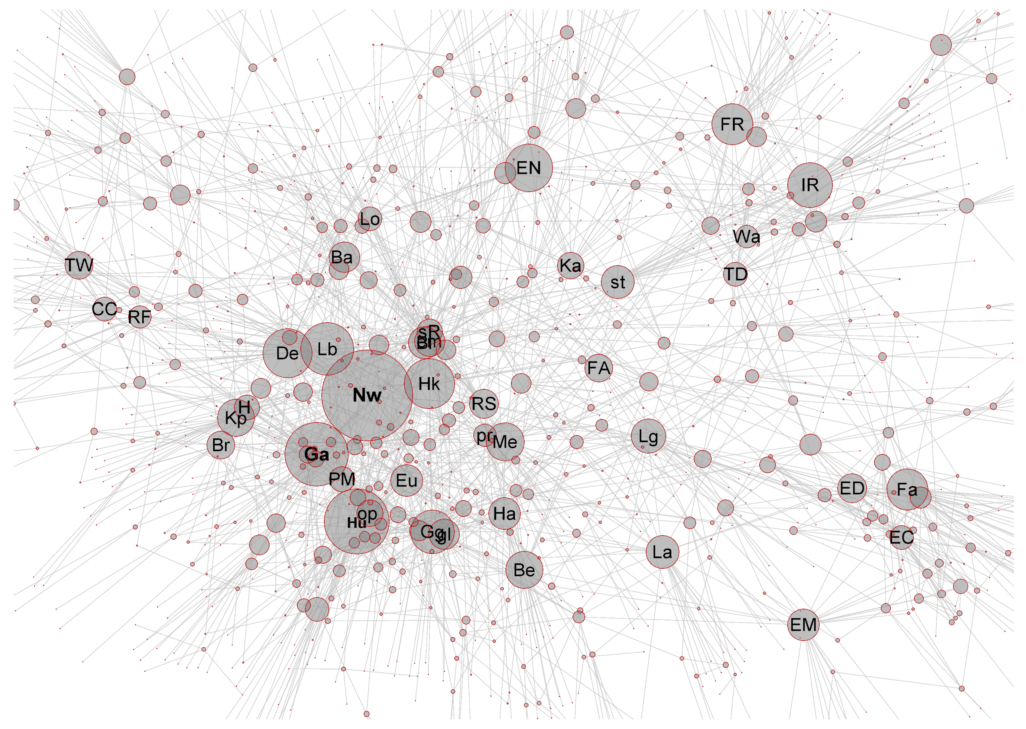
An overall visual appearance network (only the most central part) of the agglomerated AKN is shown in Figure 1, in a form of a so-called force embedded (or spring embedded) network [34,35], where most tightly connected parts are shown as the most strongly clustered regions. The nodes with the highest number of links attached to them (i.e., with degree centralities d) are persons, either scientists or scientist-philosophers. In addition, some nodes referring to scientific inventions and ideas are also among the nodes that attract many connections. These high affinity nodes, which act as kinds of hubs in the network, are listed in Table 2, with symbols referring to Figure 1. In general, the network has characteristics of a heavy-tailed complex network. The modular structure of the network [17,18] emerges from temporalisation (historical periods) as well as from thematic ordering (e.g., mechanics, thermodynamics, and electricity). Other details related to the structure of the network are discussed elsewhere [17,18].
The top 33 items (nodes) according to ranking based on the activity centrality K in the baseline model (normal diffusion) and the degrees d of nodes are summarised in Table 2. Nearly all (31) of these top ranking nodes are the same for all models of spreading activation with all choices of parameters in the range of their variation in and . Only items Boyle and Bernoulli (italicized in Table 2) are exceptions and not found among the top ranking 33 items in all models. Consequently, the top rankings are not model dependent.
In Table 3, 13 highest ranking items that are common in groups of at most of 25 highest ranking items are listed corresponding to sets obtained with different parameters and . The first two item-bands 33–46 and 47–60 in Table 3 contain all 13 items, which are always common. These items, although the relative rankings may change for different parameters and , are therefore always the common ones in all diffusion models. Taken together with results in Table 2, this indicates that about 60 highest ranking items are always the same ones, although some minor changes in their activity centrality may occur. In other groups of lower ranking items, the number of common terms in a group of 25 highest ranking terms is always less than 25, steadily decreasing with increasing index of rankings. In addition to results shown in Table 3, the next item-band 201–280 contains only six common items among 25 highest ranking ones in groups corresponding to different parameters. This indicates increasing variations in shared terms in the groups of lower ranking items. Some of the items always have the same ranking, irrespective of the model and choice of its parameters and . Most of them (shown in boldface in Table 2) are among the 25 highest ranking items or among the other relatively high ranking items (in boldface in Table 3). Only two items that retain their rankings in all models are not among the items listed in Table 2 and Table 3. Curiously, these items happen to be related to the general history of Finland and are thus of specific interest for Finnish students.
In summary, we can anticipate from the results in Table 2 and Table 3 that if only the sets of the highest ranking nodes (in Table 2) are of interest, then several not only different models but also several centrality measures provide similar rankings. This conclusion is suggested by comparison of results in Table 2 and Table 3 to results reported for the same set of data analysed by using more traditional centrality measures [18]. However, when items with lower rankings become of interest, this is not the case in general. For lower ranking items and the choices of the parameters of the model, specifying the type of spreading activation becomes of relevance. Similarly, in these cases, different centrality measures will nearly certainly produce different rankings. This behaviour is already indicated by results in Table 3. In what follows, we focus on the question of how rankings change when parameters of the mode are changed.
3.2. Changes in Rankings
The role of nodes in spreading activation is related to random walker’s return-probability on a node as well as its escape-probability from a node (see Equation (5)) at a given instant in the progress of exploration of the network. Note that, although is analogous to time, it is taken rather as a discrete external parameter that is related to the number of jumps in exploration of the network. The return and escape probabilities provide a complete enough description of the progress of exploration and the dynamic evolution of the state of the network. In what follows, we are mostly focusing on stationary states, but it is of interest to take first a closer look at how stationary states emerge from the dynamic behaviour.
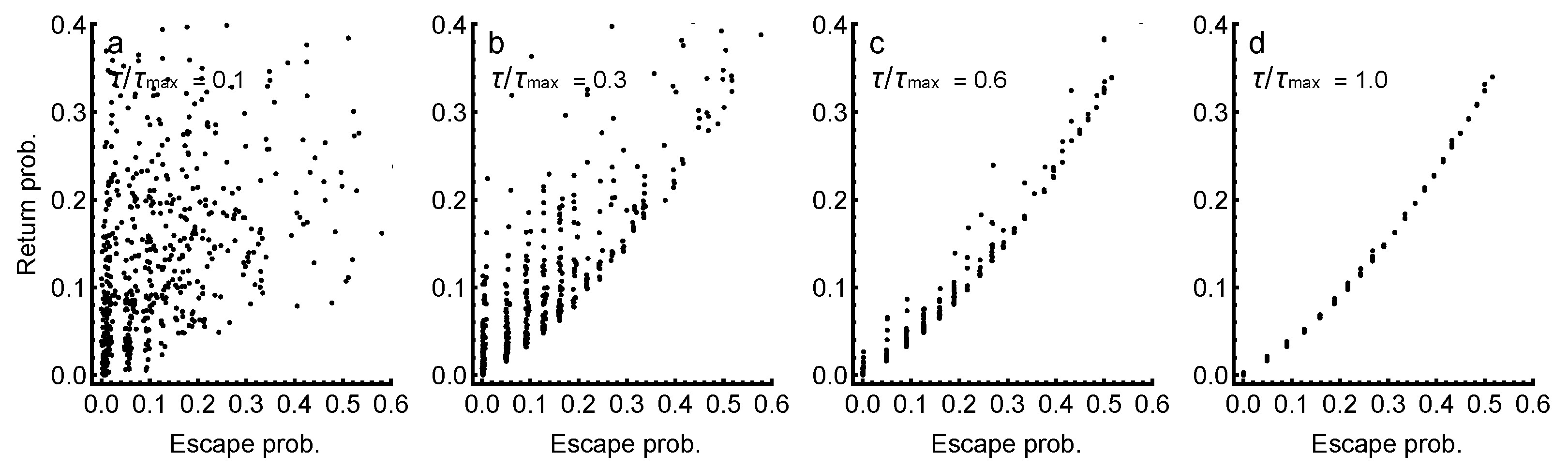
In the beginning, at small values of , the return and escape probabilities and for a given node are widely different, as is shown in Figure 2a (note that, in Figure 2, values of and are scaled to range ) for the baseline case with in . With increasing value of with progress in exploration of different routes and corresponding to a situation that many of the nodes are visited, the escape and return probabilities begin to correlate, indicating that a quasi-stationary state is reached, where the probabilities do not change appreciably. This situation is shown in Figure 2d. The overall behaviour is much the same for all diffusion models with all choices of parameters and . Differences are found only in details and a detailed shape of the final form of curve on which the results finally collapse. Consequently, the onset of correlation between values of and can be used as a proxy of stable, quasi-stationary state, in which case activity centrality K as defined in Equation (6) is an adequate measure to quantify the importance of a node in spreading activation.
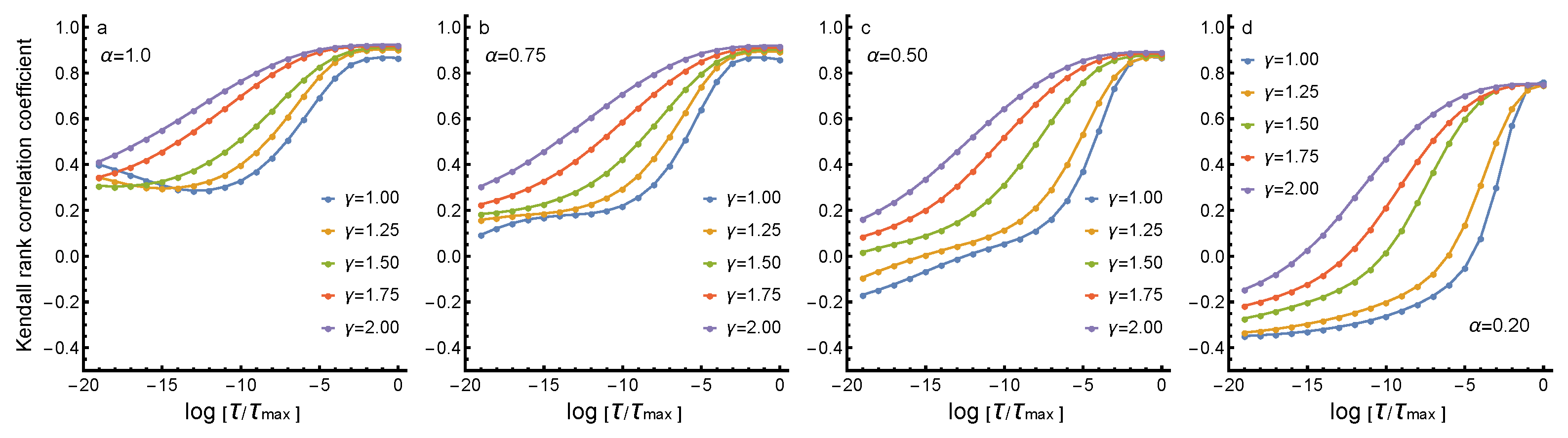
The activity centrality of nodes is different in different models of spreading diffusion corresponding to different parameter combinations . Figure 3 demonstrates the overall changes in rankings in the form of Kendall rank (tau) correlation coefficients between vectors and , where refers to values for each instant of with parameters and K refers to values at the final stationary state at of reference state with . The Kendall rank correlation coefficient is chosen because it is a nonparametric correlation test, not assuming normal distribution of data. In the present case, the distributions of differences are a centralised distribution, nearly normally distributed. The mean , standard deviation , skewness and kurtosis are initially and in the final, stationary state ; thus, the shape of the distribution of differences changes from leptokurtic to slightly platykurtic. Although differences are moderate, Kendall rank correlation as a nonparametric measure, assuming no normal distributivity, is a preferable correlation measure here (compare e.g., [44] for similar analysis in a very similar context). Moreover, the characteristic values of distribution of differences show that, although the deviations from normal distribution are systematic, they are moderate enough to rule out problems related to possible outliers (which are not detected by visual inspection either). This means that p-values for Kendall rank coefficients, as they are based on z-score like quantities, can be performed. In all cases, correlations are statistically significant with p-values smaller than and, in many cases, significantly smaller. In summary, we can conclude that correlations between K and show that, in the stationary, stable state, correlations are always substantially high, but in the beginning of evolution (as also shown in Figure 2), with , correlations are low and can be even negative, indicating that initial states of evolution are clearly different and depend on choice of the model.
In general, with low values of corresponding to the superdiffusion, the initial correlations have substantially high negative values, indicating reversed roles of nodes in spreading activity. This means that, in an initial state, nodes that eventually will have small return probabilities have initially high escape probabilities, but, in final states, a strong positive correlation between escape and return has been established (see Figure 2). This behaviour is expected because superdiffusion means more effective and nonlocal exploration of available paths, and thus diversity in paths explored. With increasing value of , the correlations are systematically higher, indicating that increased nonlinearity counterbalances the diversity of paths explored. In continuum diffusion models, the paralleling effect is a formation of a boundary layer of diffusion when nonlinearity is increased. However, in all cases, in the final states, high positive correlations with the reference state is achieved, with very small differences in the limiting value of correlations.
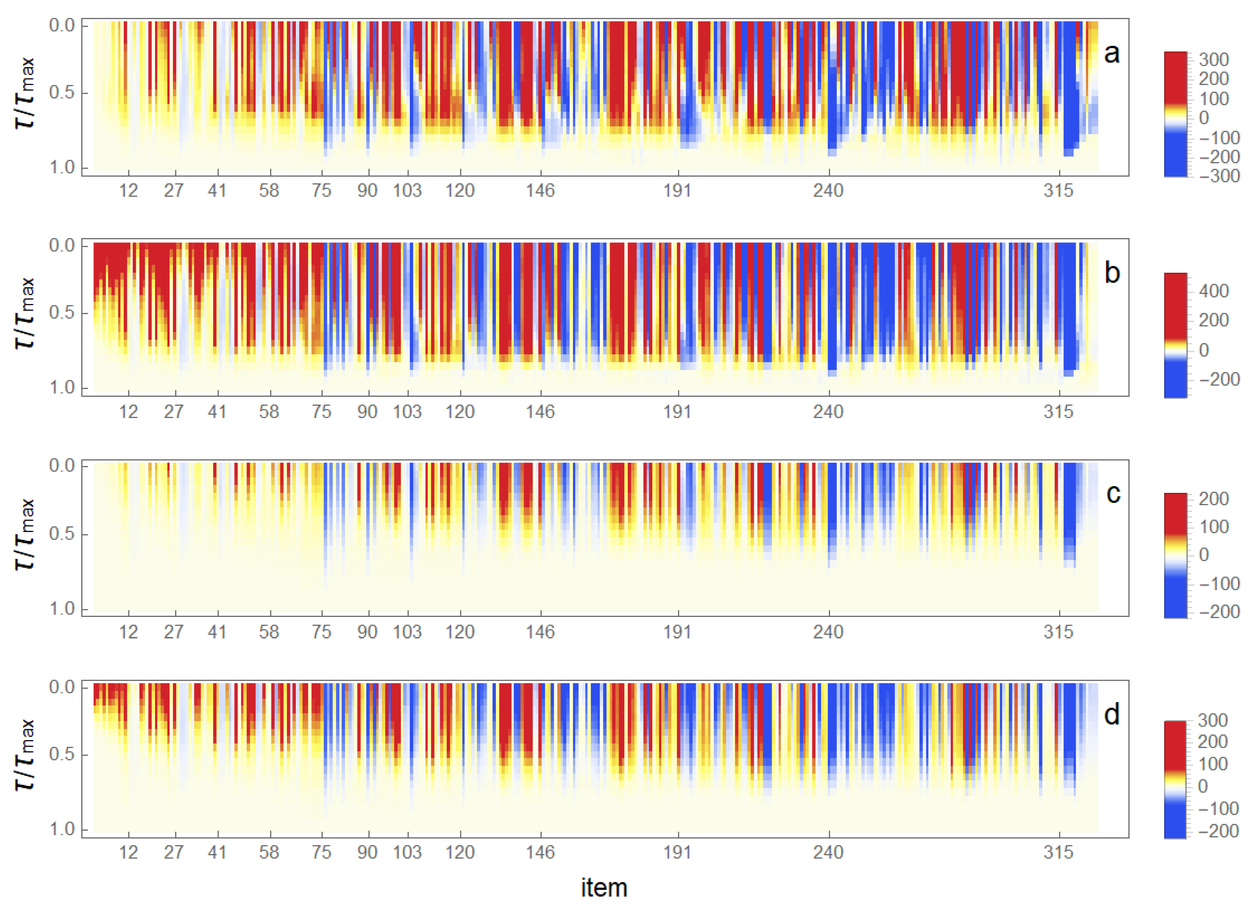
The activity centrality of the item (node) is a basis to form rankings; the higher the value, the higher the ranking of the item. As we have seen, activity of a node may change substantially during the evolution towards the stable state. In Figure 4, how rankings of items from 1 to 330 change during evolution is shown in the case of four different models A–D corresponding to different parameters . The cases are A (), B (), C () and D (). In all cases, evolution is shown as a function of , where depends on parameter choices being larger, the larger the values of and are. In Figure 4, the evolution towards the final stable state is shown and, therefore, the reference state is chosen to be the final stable state in each choice of parameters, meaning that final states at are slightly different in cases A–D.
In Figure 4, we observe that, for model A with = (1,1), evolution towards the final stable state occurs for some nodes with rather random-like changes in rankings. These nodes are sometimes increasing and sometimes decreasing their rankings. The more stable bands where neighbouring items behave similarly, either with an increase or decrease of rankings, are visible—for example, blue bands starting at locations marked in figures, and red bands located between them. With lower value of parameter = 0.5 in model B, the random-like changes between increase and decrease in ranking becomes moderated, but otherwise the behaviour remains much the same. The most important difference is that, in model B, the value of is smaller roughly by a factor of 100 in comparison to model A. This is as expected because low values of correspond to superdiffusive behaviour and thus faster relaxation to a stable state.
The situation shown for model A in Figure 4 changes when the value of parameter is increased. Values correspond to a situation that is analogous to diffusion in continuous porous or fractal medium, where diffusivity itself depends on density profiles of diffusing substance, i.e., here, on occupation of node as expressed by Equation (3). Such a nonlinearity in continuous diffusion leads to the formation of boundary layer in a diffusion front [30,31,32]. Here, an analogous effect in the case of models C and D with = 1.75 is more pronounced formation of bands of increasing (red bands) and decreasing (blue bands), which are more clearly bunched than in cases A and B where = 1.0. A similar effect of nonlinearity was already found in the previous study where sub-structures of the associative network were in focus [17]. The increase in nonlinearity by an increase in value of parameter thus enhances the tendency that neighbouring nodes behave in a similar way and thus sharp boundaries between such regions are formed. Moreover, as shown by comparing cases B and D to cases A and C, the effect of reducing the value of (i.e., moving towards superdiffusion) appears to enhance in a similar way the formations of consolidated band-like structure; there is a segregation of regions where rankings increase from regions where it decreases. Finally, in all cases A–D, it interesting that there are borderlines, where one finds no crossings from increase to decrease in rankings. Some such borderlines are indicated in Figure 5. It is also seen that the high-activity nodes with high rankings in regions from 1 to about 35 are stabilised earlier than others and thus their rankings do not change in further evolution (see Table 2 and Table 3 for a summary of the stable items).
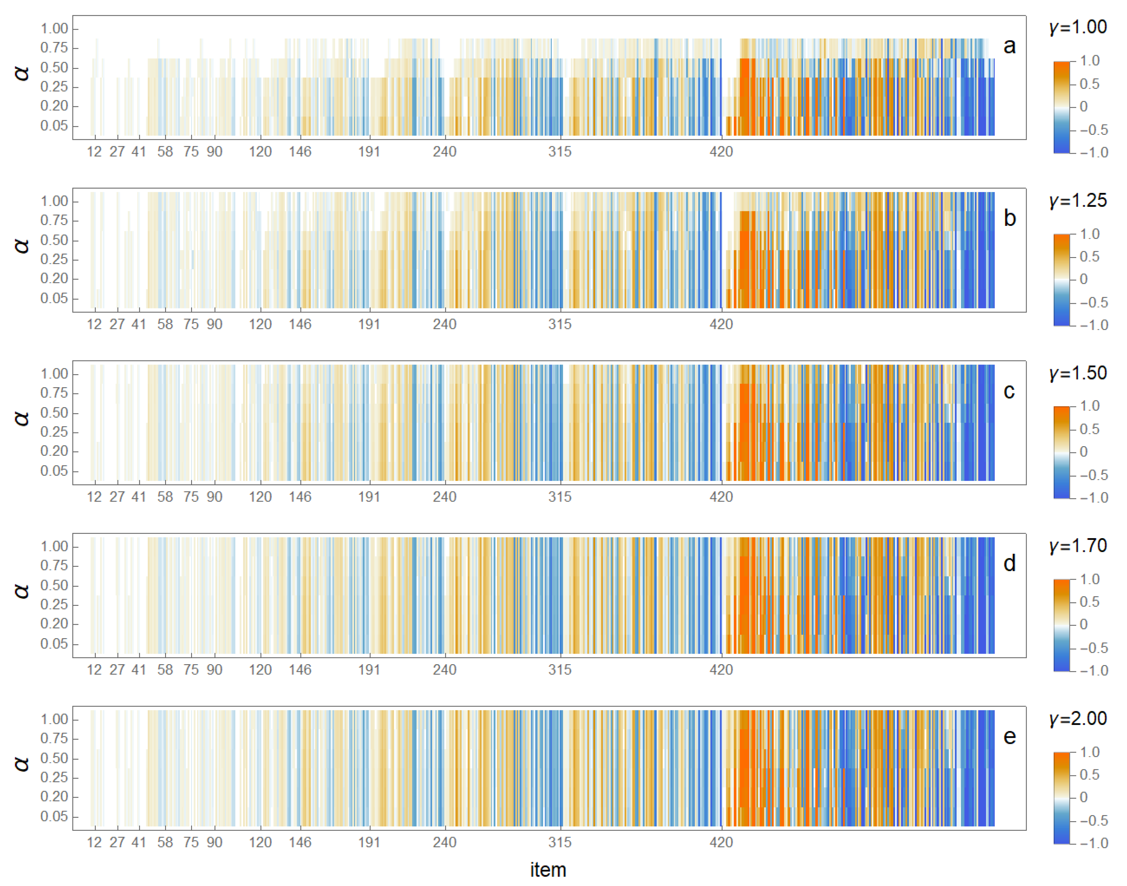
The rankings in final stationary state in different models are compared in Figure 5. In this case, the reference state is the same one in all cases, corresponding to the model A in Figure 4 with parameters with = (1,1). In Figure 5, the five panels (a–e) show cases for increasing nonlinearity, with: = 1.0 (a); 1.25 (b); 1.50 (c); 1.75 (d) and 2.00 (e). In each of the cases (a–e), six different cases of diffusion (in order of increasing superdiffusion) are shown, with: =1.0, 0.75, 0.50, 0.25, 0.20, and 0.05. It is now seen that, in the case of about 40, the highest ranking items the rankings are essentially similar; choice of model does not make any difference if only these highest ranking items are of interest. The item ranks marked in Figure 5 (as well as in 4) correspond to different degrees, with the highest degree d in the end of band given in form R(d) as follows: 12(23); 27(19); 41(16); 58(13); 75(11); 90(9); 120(8); 146(7); 191(6); 240(5); 315(4); 420(3). The items with ranks 421–597 have only a minimum number of two links (the network includes only the 2-core of total network of about 1200 nodes).
In the case of items with intermediate rankings from 41 to 146, changes in rankings start to appear but yet remain moderate. In the region of ranks from 1 to 40, the degrees of nodes corresponding to different items are relatively high, rank 1 of item Newton with d = 64 to rank 40 with d = 16 of item Scientific method. The next band of items from 147 up to 240 has a more pronounced change in rankings, occurring in clear bands. With lower rankings and lower degrees, changes become more common, and nearly all items eventually change rankings. The largest changes of rankings in the band from 241 up to 597 are about ±150, meaning quite large differences in rankings for different models. In all cases, however, the degree of nodes constrains the changes in rankings, and, generally (although not exactly), changes in rankings occur within bands of constant degrees and only a few border crossings between different bands occur.
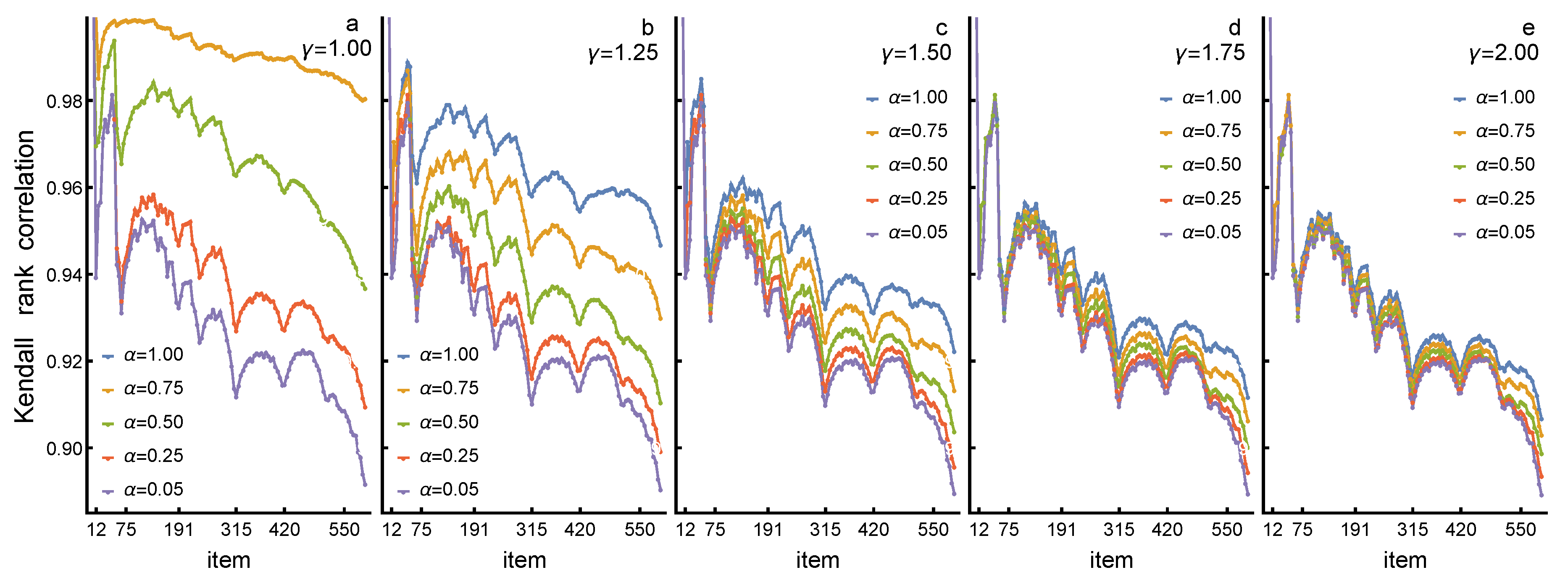
Complementary information of the changes in rankings and formation of banded structure associated with it is obtained when we form cumulative sums of the changes in rankings. In Figure 4 and Figure 5, red bands indicate increase in ranking while blue bands indicate decrease. In cumulative sums of the changes in rankings, we then observe regions, where the cumulative sum of the changes steadily increases, reaching a maximum and then begins to decrease. Figure 6 shows Kendall rank correlations of cumulative sums of the changes in rankings for final stationary states for in different models (a)–(e) shown in Figure 5. Here, as in the case of results in Figure 3, the Kendall rank correlation coefficient is preferred (compare also [44]). The distributions of differences in rankings and of item i (as based on corresponding activity centralities and ) and given by are again centralised distribution. The mean, standard deviation, skewness and kurtosis and their bounds of variations are different in different item-bands as follows: for items ; for items ; and for items . In summary, the changes in rankings increase steadily with lowering of rankings (i.e., increasing value of i), while the distribution of is only slightly skewed but remains clearly leptokurtic throughout. In all cases (with similar arguments as discussed in context of Figure 3), correlations are statistically significant with p-values smaller than and, in many cases, significantly lower. Correlations are relative to rankings in baseline model (a) (or A in Figure 4) with = (1,1). For model (a) with = 1.0, we see that different values of < 1 for enhanced diffusion produce clearly different rankings, indicated as different Kendall rank correlation that decreases with decreasing rank and increasing superdiffusion (i.e., decreasing value of ). However, up to about rank 40, with only a few exceptions, correlations are high, indicating once again that highest ranks remain intact. The banded structure is now very clearly visible as oscillations in cumulative sums, minima located at the boundaries of bands (border between red and blue bands in Figure 4 and Figure 5).
Interestingly, when nonlinearity is increased by increasing the value of parameter , we observe that all correlations begin to approach the limiting correlations obtained with the lowest values of = 0.05, obviously representing limit . In addition, in model (e) with the highest nonlinearity, = 2.0 correlations (and thus rankings in that model) are the same for all values of and correspond to the highest attainable superdiffusion. In a sense, this is the most stable limiting case and the most different in comparison to the baseline model.
Results in Figure 6 show clearly that, with lower rankings, correlations decrease, meaning that increasingly more changes occur with increasingly lower rankings, and that a different choice of diffusion models produces clearly different rankings for items with rankings from 60–70 onwards, while higher ranks from 1 to about 35–40 remain much the same in all models. The largest relative changes in rankings (i.e., the largest differences in correlations between peaks and valleys in correlation curves) are obtained either with the most efficient superdiffusion (the lowest values of ) or with the strongest effect of nonlinearity (the highest value of ). Moreover, in these cases, correlations in the changes in ranking are very similar. Obviously, superdiffusion and nonlinear dependence both enhance the effect of exploring the network more effectively; superdiffusion finding faster remotely connected nodes but yet importance in spreading activation, nonlinearity putting weight on these same nodes through nonlinear weighting. The combined effect, as shown by results in Figure 4 and Figure 5 as well as in Figure 6, is strong segregation into groups where rankings either diminish or increase.
4. Discussion
We have introduced here a model that embodies and quantifies the spreading activation theory related to exploration of semantic networks, in particular as it has been applied in describing the associative knowledge networks (AKNs) [10,11,12]. The core idea of conventional models of spreading activation is an assumption that activation of nodes in AKNs is a diffusion-like or Brownian random walk process [4,13,14,16]. However, the assumption that only conventional diffusion or a Brownian random walk should be of interest for AKNs is restrictive and not necessarily the best option from the point of view that what is known about cognitive processes spreading activation is meant to describe. For example, there is little reason to assume that routes or paths are accessible only through sequential jumps between links, thus ruling out easy and fast association between items separated by longer paths. Moreover, one may expect that probability of occupation of given node during the diffusion or random walk process may depend on the occupation probability nonlinearly, like a diffusion in fractal or porous medium [30,31,32]. To generalise spreading activation models, we proposed a model inspired by recent advances in modelling dynamic processes in complex networks, by taking into account the possibility of nonlocal diffusion (superdiffusion) and nonlinearity of the diffusion process.
The generalised model introduced here is based on graph Laplacian, usually used in description of complex networks and in finding its key nodes and their rankings. The graph Laplacian is the basic quantity in describing random walk in a network by using only matrix transformations. This is analogous to describing ordinary diffusion by using a partial differential equation and Laplace operator (therefore the name graph Laplacian) [34,35]. The graph Laplacian was normalized to relax the constraint on conserved flows, which is restrictive and not necessarily tenable for modelling (non-substantial and non-physical) flows of interest for spreading activation. This modification is similar to that used to obtain so-called quantum-PageRank, providing a more holistic exploration of the network than the ordinary PageRank [19,20,21]. The superdiffusive spreading, on the other hand, was modelled by introducing the fractional form of normalized graph Laplacian [25,26,27]. The fractional graph Laplacian is analogous to fractional Laplace-operator in fractional calculus, used to model superdiffusion in continuum diffusion models [30,31,32]. In addition, the nonlinearity of the diffusion model was shown to lead to a general solution in a form q-generalized adjacency kernel [33], which can be then adopted as a generalized systemic state describing the network in spreading activation (compare with [17]). The resulting model and systemic state as its solution is then analogous to a fractional porous medium diffusion (FPMD) equation applied to model anomalous diffusion in continuous (but heterogeneous or porous) medium [30,31,32].
Interestingly, models that share many similarities with the model proposed here have been utilized to model human–machine control processes and human operator systems, and feedback and memory effects related to them [45,46]. Although such contexts differ from the context, where spreading activation is of interest, in both cases, one can recognise the role of making choices, memory of encountered states during the process, and how cues affect choices and decisions made. In the present context, many such factors underlie not only the formation of the structure of network but also the dynamics of how choices are made between different paths or routes to progress in that network. For future research, the approach on spreading activation making use of control systems theory utilizing fractional Laplacian operators [45,46] might be an interesting avenue to pursue.
The proposed generalized model of spreading activation and activity centrality in forming the rankings was explored here in the case of AKN based on university students’ knowledge about the history of science, recently explored by using static centrality measures [18] as well as the role of sub-networks in spreading activation [17]. The analysis based on spreading activation presented here shows that, for nodes that have a high degree and high centrality in terms of traditional measures, all variants of spreading activation models, from ordinary diffusion to superdiffusion, produce essentially similar results for the ranking of nodes. However, nodes with intermediate rankings and lower, different choices of the diffusion model produce very different rankings. For these nodes, a question about how to motivate the choice of the diffusion model becomes of importance and needs to be justified; a Brownian model is by no means an obvious preferred choice. Interestingly, in all cases, the node degrees determine bands on within rankings change and very few border crossings across the bands are observed.
Finally, we note that recent research in learning and education utilizing network approaches offer many similar educational contexts of applications as discussed here (see, e.g., [47,48] and references therein). In particular, networks that are very similar to the AKN studied here have recently been examined in learning physics [49,50,51,52], chemistry [53], computer science and statistics [54,55] as well as in learning psychology and education [56,57] and the history of science [58,59]. In these cases, network measures used in analysis have been conventional static and local centrality measures. However, in all mentioned cases, analysis based on spreading activation can be expected to provide results showing interesting differences when compared to methods using the conventional centrality measures as used thus far.
5. Conclusions
The model proposed is based on a fractional normalized graph Laplacian and a generalised nonlinear diffusion equation, which generalises ordinary diffusion to a nonlocal superdiffusive behaviour, and, with a nonlinearity, enhancing the role of nodes that have important dynamic roles in spreading activation. The major theoretical results of the study are: (1) a generalised model based on fractional graph Laplacian for spreading activation in a complex network; (2) a general matrix transformation in the form of q-adjacency kernel that solves the model and provides the systemic state describing spreading activation; and (3) the activity centrality for ranking of nodes according to their importance in spreading activation. The systemic state is a well-defined matrix transformation for a parameter region that spans the superdiffusive region and a region of strong nonlinearity. In that, the systemic state is analogous to an analytic solution of fractional porous diffusion equations.
The viability of the suggested model in the description of spreading activation and uses of activity centrality in forming the rankings was demonstrated by using one specific associative knowledge network, a recently studied case in the context of teaching and learning the history of science [18]. The results showed that, if only highest ranking nodes are of interest, the specific details of the model are not crucial, but details of choosing the diffusion model become of importance for intermediate and low ranking nodes. This behaviour demonstrates that paying attention to the choice of model for spreading activation is a crucial question, essentially affecting how ranking and importance of nodes are evaluated. Consequently, the question of choosing a particular model is a theoretical decision of what kinds of features—locally available or those also available through nonlocal and nonlinear diffusion processes—are of interest in forming rankings of the nodes.
Funding
This research was funded by Academy of Finland Grant No. 311449.
Institutional Review Board Statement
Not applicable.
Informed Consent Statement
Not applicable.
Data Availability Statement
The data supporting this study are from previously reported studies, which have been cited.
Conflicts of Interest
The author declares no conflict of interest.
References
- Sowa, J.F. Semantic networks. In Encyclopedia of Cognitive Science; Nadel, L., Ed.; John Wiley & Sons: New York, NY, USA, 2006. [Google Scholar]
- Hartley, R.T.; Barnden, J.A. Semantic networks: Visualizations of knowledge. Trends Cogn. Sci. 1997, 1, 169–175. [Google Scholar] [CrossRef] [Green Version]
- Lehmann, F. Semantic networks. Comput. Math. Appl. 1992, 23, 1–50. [Google Scholar] [CrossRef] [Green Version]
- Siew, C.S.Q.; Wulff, D.U.; Beckage, N.M.; Kenett, Y.N. Cognitive Network Science: A Review of Research on Cognition through the Lens of Network Representations, Processes, and Dynamics. Complexity 2019, 2019, 2108423. [Google Scholar] [CrossRef]
- Siew, C.S.Q. Applications of Network Science to Education Research: Quantifying Knowledge and the Development of Expertise through Network Analysis. Educ. Sci. 2020, 10, 101. [Google Scholar] [CrossRef] [Green Version]
- Kenett, Y.N.; Beckage, N.M.; Siew, C.S.Q.; Wulff, D.U. Editorial: Cognitive Network Science: A New Frontier. Complexity 2020, 2020, 6870278. [Google Scholar] [CrossRef]
- Koponen, I.T.; Mäntylä, T. Editorial: Networks Applied in Science Education Research. Educ. Sci. 2020, 10, 142. [Google Scholar] [CrossRef]
- De Deyne, S.; Kenett, Y.N.; Anaki, D.; Faust, M.; Navarro, D. Large-scale network representations of semantics in the mental lexicon. In Frontiers of Cognitive Psychology. Big Data in Cognitive Science; Jones, M.N., Ed.; Routledge/Taylor & Francis Group: Abingdon, UK, 2017; pp. 174–202. [Google Scholar]
- Steyvers, M.; Tenenbaum, J.B. The Large-Scale Structure of Semantic Networks: Statistical Analyses and a Model of Semantic Growth. Cogn. Sci. 2005, 29, 41–78. [Google Scholar] [CrossRef]
- Collins, A.M.; Loftus, E.F. A spreading-activation theory of semantic processing. Psychol. Rev. 1975, 82, 407–428. [Google Scholar] [CrossRef]
- Lerner, I.; Bentin, S.; Shriki, O. Spreading Activation in an Attractor Network With Latching Dynamics: Automatic Semantic Priming Revisited. Cogn. Sci. 2012, 36, 1339–1382. [Google Scholar] [CrossRef] [Green Version]
- Hills, T.T.; Jones, M.N.; Todd, P.M. Optimal Foraging in Semantic Memory. Psychol. Rev. 2012, 119, 431–440. [Google Scholar] [CrossRef] [Green Version]
- Abbott, J.T.; Austerweil, J.L.; Griffiths, T.L. Random Walks on Semantic Networks Can Resemble Optimal Foraging. Psychol. Rev. 2015, 122, 558–569. [Google Scholar] [CrossRef] [PubMed]
- Kenett, Y.N.; Levi, E.; Anaki, D.; Faust, M. The Semantic Distance Task: Quantifying Semantic Distance With Semantic Network Path Length. J. Exp. Psychol. 2017, 43, 1470–1489. [Google Scholar] [CrossRef]
- Siew, C.S.Q. Spreadr: An R package to simulate spreading activation in a network. Behav. Res. Meth. 2019, 51, 910–929. [Google Scholar] [CrossRef] [Green Version]
- Griffiths, T.L.; Steyvers, M.; Firl, A. Google and the Mind: Predicting Fluency With PageRank. Psychol. Sci. 2007, 18, 1069–1076. [Google Scholar] [CrossRef]
- Koponen, I.T. Systemic States of Spreading Activation in Describing Associative Knowledge Networks: From Key Items to Relative Entropy Based Comparisons. Systems 2021, 9, 1. [Google Scholar] [CrossRef]
- Koponen, I.; Nousiainen, M. University students’ associative knowledge of history of science: Matthew effect in action? Eur. J. Sci. Math. Educ. 2018, 6, 69–81. [Google Scholar] [CrossRef]
- Biamonte, J.; Faccin, M.; De Domenico, M. Complex networks from classic to quantum. Commum. Phys. 2019, 2, 53. [Google Scholar] [CrossRef] [Green Version]
- Faccin, M.; Johnson, T.; Biamonte, J.; Kais, S.; Migdał, P. Degree Distribution in Quantum Walks on Complex Networks. Phys. Rev. X 2013, 3, 041007. [Google Scholar] [CrossRef] [Green Version]
- Paparo, D.P.; Müller, M.; Comellas, F.; Martin-Delgado, M.A. Quantum Google in a Complex Network. Sci. Rep. 2013, 3, 2773. [Google Scholar] [CrossRef] [Green Version]
- Garnerone, S. Thermodynamic formalism for dissipative quantum walks. Phys. Rev. A 2012, 86, 032342. [Google Scholar] [CrossRef] [Green Version]
- De Domenico, M.; Biamonte, J. Spectral Entropies as Information-Theoretic Tools for Complex Network Comparison. Phys. Rev. X 2016, 6, 041062. [Google Scholar] [CrossRef] [Green Version]
- Mülken, O.; Blumen, A. Continuous-time quantum walks: Models for coherent transport on complex networks. Phys. Rep. 2011, 502, 37–87. [Google Scholar] [CrossRef] [Green Version]
- Riascos, A.P.; Mateos, J.L. Fractional dynamics on networks: Emergence of anomalous diffusion and Lévy flights. Phys. Rev. E 2014, 90, 032809. [Google Scholar] [CrossRef] [PubMed] [Green Version]
- Riascos, A.P.; Mateos, J.L. Long-range navigation on complex networks using Lévy random walks. Phys. Rev. E 2012, 86, 056110. [Google Scholar] [CrossRef] [Green Version]
- Benzi, M.; Bertaccini, D.; Durastante, F.; Simunec, I. Non-local network dynamics via fractional graph Laplacians. J. Complex Netw. 2020, 8, cnaa017. [Google Scholar] [CrossRef]
- Estrada, E.; Hameed, E.; Hatano, N.; Langer, M. Path Laplacian operators and superdiffusive processes on graphs. I. One-dimensional case. Linear Algebra Appl. 2017, 523, 307–334. [Google Scholar] [CrossRef] [Green Version]
- Estrada, E.; Hameed, E.; Langer, M.; Puchalska, A. Path Laplacian operators and superdiffusive processes on graphs. II. Two-dimensional lattice. Linear Algebra Appl. 2018, 555, 373–397. [Google Scholar] [CrossRef] [Green Version]
- de Pablo, A.; Quirós, F.; Rodríguez, A.; Vázquez, J.L. A fractional porous medium equation. Adv. Math. 2011, 226, 1378–1409. [Google Scholar] [CrossRef] [Green Version]
- Vázquez, J.L. Recent progressin the theory of nonlinear diffusion with fractional Laplacian operators. Discret. Cont. Dyn. Syst. Ser. S 2014, 7, 857–885. [Google Scholar]
- Bologna, M.; Tsallis, C.; Grigolini, P. Anomalous diffusion associated with nonlinear fractional derivative Fokker–Planck-like equation: Exact time-dependent solutions. Phys. Rev. E 2000, 62, 2213–2218. [Google Scholar] [CrossRef] [Green Version]
- Koponen, I.T.; Palmgren, E.; Keski-Vakkuri, E. Characterising heavy-tailed networks using q-generalised entropy and q-adjacency kernels. Physica A 2021, 566, 125666. [Google Scholar] [CrossRef]
- Estrada, E. The Structure of Complex Networks: Theory and Applications; Oxford University Press: Oxford, UK, 2012. [Google Scholar]
- Newman, M.E.J. Networks: An Introduction; Oxford University Press: Oxford, UK, 2010. [Google Scholar]
- Tsallis, C. Introduction to Nonextensive Statistical Mechanics: Approaching a Complex World; Springer: New York, NY, USA, 2009. [Google Scholar]
- Tsallis, C. Economics and Finance: Q-Statistical Stylized Features Galore. Entropy 2017, 19, 457. [Google Scholar] [CrossRef] [Green Version]
- Borges, E.P. On a q-generalization of circular and hyperbolic functions. J. Phys. A Math. Gen. 1998, 31, 5281–5288. [Google Scholar] [CrossRef]
- Yamano, T. Some properties of q-logarithm and q-exponential functions in Tsallis statistics. Physica A 2002, 305, 486–496. [Google Scholar] [CrossRef]
- Ferri, G.L.; Martinez, S.; Plastino, A. Equivalence of the four versions of Tsallis’s statistics. J. Stat. Mech. 2005, 2005, P04009. [Google Scholar] [CrossRef] [Green Version]
- Kunegis, J.; Fay, D.; Bauckhage, C. Spectral evolution in dynamic networks. Knowl. Inf. Syst. 2013, 37, 1–36. [Google Scholar] [CrossRef]
- Benzi, M.; Klymko, C. On the Limiting Behavior of Parameter-Dependent Network Centrality Measures. SIAM J. Matrix Anal. Appl. 2015, 36, 686–706. [Google Scholar] [CrossRef] [Green Version]
- Brin, S.; Page, L. The anatomy of a large-scale hypertextual Web search engine. Comput. Netw. ISDN Syst. 1998, 30, 107–117. [Google Scholar] [CrossRef]
- Sanchez-Burillo, E.; Duch, J.; Gomez-Gardenes, J.; Zueco, D. Quantum Navigation and Ranking in Complex Networks. Sci. Rep. 2012, 2, 605. [Google Scholar] [CrossRef] [Green Version]
- Martínez-García, M.; Gordon, T.; Shu, L. Extended Crossover Model for Human-Control of Fractional Order Plants. IEEE Access 2017, 5, 27622–27635. [Google Scholar] [CrossRef]
- Martínez-García, M.; Zhang, Y.; Gordon, T. Memory Pattern Identification for Feedback Tracking Control in Human–Machine Systems. Hum. Factors 2021, 63, 210–226. [Google Scholar] [CrossRef] [Green Version]
- Ifenthaler, D.; Hanewald, R. Digital Knowledge Maps in Education:Technology-Enhanced Support for Teachers and Learners; Springer: New York, NY, USA, 2014. [Google Scholar]
- Nesbit, J.C.; Adesope, O.O. Learning with Concept and Knowledge Maps: A Meta-Analysis. Rev. Educ. Res. 2006, 76, 413–448. [Google Scholar] [CrossRef] [Green Version]
- Kubsch, M.; Touitou, I.; Nordine, J.; Fortus, D.; Neumann, K.; Krajcik, J. Transferring Knowledge in a Knowledge-in-Use Task -Investigating the Role of Knowledge Organization. Educ. Sci. 2020, 10, 20. [Google Scholar] [CrossRef] [Green Version]
- Thurn, M.; Hänger, B.; Kokkonen, T. Concept Mapping in Magnetism and Electrostatics: Core Concepts and Development over Time. Educ. Sci. 2020, 10, 129. [Google Scholar] [CrossRef]
- Koponen, I.T.; Nousiainen, M. Concept networks of students’ knowledge of relationships between physics concepts: Finding key concepts and their epistemic support. Appl. Netw. Sci. 2018, 3, 14. [Google Scholar] [CrossRef] [Green Version]
- Koponen, I.T.; Nousiainen, M. Pre-service physics teachers’ understanding of the relational structure of physics concepts: Organising subject contents for purposes of teaching. Int. J. Sci. Math. Educ. 2013, 11, 325–357. [Google Scholar] [CrossRef]
- Derman, A.; Eilks, I. Using a word association test for the assessment of high school students’ cognitive structures on dissolution. Chem. Educ. Res. Pract. 2016, 17, 902–913. [Google Scholar] [CrossRef]
- Vukic, D.; Martincic-Ipsic, S.; Mestrovic, A. Structural Analysis of Factual, Conceptual, Procedural, and Metacognitive Knowledge in a Multidimensional Knowledge Network. Complexity 2020, 2020, 9407162. [Google Scholar] [CrossRef]
- Kapuza, A. How Concept Maps with and without a List of Concepts Differ: The Case of Statistics. Educ. Sci. 2020, 10, 91. [Google Scholar] [CrossRef] [Green Version]
- Siew, C.S.Q. Using network science to analyze concept maps of psychology undergraduates. Appl. Cogn. Psychol. 2019, 33, 662–668. [Google Scholar] [CrossRef]
- Koponen, M.; Asikainen, M.; Viholainen, A.; Hirvonen, P. Using network analysis methods to investigate how future teachers conceptualize the links between the domains of teacher knowledge. Teach. Teach. Educ. 2019, 79, 137–152. [Google Scholar] [CrossRef]
- Lommi, H.; Koponen, I.T. Network cartography of university students’ knowledge landscapes about the history of science: Landmarks and thematic communities. Appl. Netw. Sci. 2019, 4, 6. [Google Scholar] [CrossRef]
- Alcantara, M.C.; Braga, M.; van den Heuvel, C. Historical Networks in Science Education: A Case Study of an Experiment with Network Analysis by High School Students. Sci. Educ. 2020, 29, 101–121. [Google Scholar] [CrossRef]
Figure 1.
The agglomerated AKN representing students’ associative knowledge of the history of science. Only the most central part of the network is shown for better visibility. The size of the nodes is proportional to the degree d (i.e., number of links attached) of the node. The abbreviations are explained in Table 2.

Figure 2.
Scatter plots of return and escape probabilities and (scaled in range with increasing values of scaled to maximum , with =0.1 (a), 0.3 (b), 0.6 (c) and 1.0 (d). The cases shown are for a baseline model with and . Stabilization of spreading activation is obtained when correlation between escape and return probabilities becomes high and results collapse onto a single regular curve (Figure 2d).

Figure 3.
Kendall rank correlation coefficients between vectors and , where refers to values for each instant of with parameters and K to values at the final stationary state at of reference state with . Results are shown for 1.0 (a), 0.75 (b), 0.50 (c) and 0.20 (d). Different parameter combinations are indicated in figure legends. In all cases, p-values for correlations are below .

Figure 4.
Fingerprint maps of changes in rankings (based on activity centrality K) of items 1–330 for different models corresponding parameters: (a) (); (b) (); (c) (); and (d) (). The decrease in rankings is in blue and the increase in red, while white regions correspond to changes in rankings, which are low in comparison to reference state (final state of model A). The bar legend explains the colour coding.

Figure 5.
Fingerprint maps of changes in rankings (based on activity centrality K) of all items 1–597 for a range of values =1.0, 0.75, 0.50, 0.25, 0.20 and 0.05 and = 1.0 (a); 1.25 (b); 1.50 (c); 1.75 (d) and 2.00 (e). The decrease in rankings is in blue and the increase in red, while regions in light colours correspond to changes in rankings, which are low in comparison to the reference state (final state of model A). The bar legends at right explain the colour coding. Changes in rankings are normalized to a maximum of 150.

Figure 6.
Kendall rank correlations of cumulative sums in changes in rankings as correlated to baseline model (a) in Figure 5 (or a in Figure 4) with = (1,1). Results shown are averaged over seven nodes. In all cases, p-values are below .


Table 1.
A schematic representation of the generalized model. In a network, where nodes are connected through adjacency matrix , direct jumps are restricted to sites connected by links (solid lines). Long jumps occur between distant nodes, when the fractional graph Laplacian (F.g. Laplacian) has a nonzero element between nodes that are not directly connected (), but connected through intermediate steps (two examples shown by a dashed line). Then, the systemic state also has non-zero elements between the nodes and allowing spreading activation between the nodes. The function is the generalised q-exponential.
| Scheme of Long Jumps | Description | Symbol |
|---|---|---|
 | Adjacency matrix | |
| Elements of | ||
| Degree matrix | ||
| Graph Laplacian | ||
| F. g. Laplacian | ||
| Elements of | ||
| Systemic state | ||
| Elements of |
Table 2.
Rankings of the highest ranking 33 items and their degree d. Ranking is based activity centrality K in the case of normal diffusive spreading corresponding to parameters and . Acronyms (Ac) refer to Figure 1. The items that have the same rankings in all models with different parameters and are in boldface.
| Item | d | Ac | Item | d | Ac | Item | d | Ac |
|---|---|---|---|---|---|---|---|---|
| 1. Newton | 64 | Nw | 12. Bernoulli | 23 | Be | 23. Optics | 20 | op |
| 2. Galilei | 44 | Ga | 13. Faraday | 22 | Fa | 24. Bacon | 20 | Ba |
| 3. Huygens | 41 | Hu | 14. Electrodynamics | 22 | EM | 25. Scientific revol. | 20 | sR |
| 4.Hooke | 36 | Hk | 15. Industrial revol. | 22 | IR | 26. Brahe | 19 | Br |
| 5. Leibniz | 32 | Lb | 16. Kepler | 22 | Kp | 27. Planet motion | 19 | PM |
| 6. Descartes | 31 | De | 17. Gravitation law | 22 | gl | 28. Euler | 19 | Eu |
| 7. Gravitation | 30 | Gg | 18. Steam engine | 22 | st | 29. Electric current | 18 | EC |
| 8. Enlightenment | 29 | EN | 19. Royal Society | 22 | RS | 30. Electricity | 18 | ED |
| 9. Mechanics | 27 | Me | 20. French revol. | 21 | FR | 31. Thermodynamics | 18 | TD |
| 10. Empiricism | 23 | em | 21. French Academy | 21 | FA | 32. Reformation | 17 | RF |
| 11. Boyle | 23 | Bo | 22. Heliocentricity | 20 | H | 33. Locke | 17 | Lo |
Table 3.
Summary of 13 highest ranking items based on activity centrality K calculated for reference case with parameters and . The 13 items shown are common in sets 25 of the highest ranking in a given band I–V of items and with all parameters in and . The total number of shared items out of the 25 highest ranking items are given in parenthesis in form (shared/all). Numbering of items is based on the reference case. The items that have the same rankings in all models with different parameters and are in boldface. Abbreviations refer to Figure 1.
| Key Items in Item Bands I–V | ||||
|---|---|---|---|---|
| I 33–46 (13/13) | II 47–60 (13/13) | III 61–100 (20/25) | IV 101–140 (18/25) | V 141–200 (16/25) |
| Locke (Lo) | Thermometer | Beeckman | Finnish War | Thought experim. |
| Halley (Ha) | Volta | Wave thr. light | Electric potential | Chatelet |
| Watt (Wa) | Earth magn field | Atmsph. pressure | Kirchhoff | Medical science |
| Cath. church (CC) | Stevin | Telescope | Hydrost. pressure | Gauss |
| Pressure (pr) | Ludvig XIV | Fire of London | Gay-Lussac law | Mozart |
| Laplace (LP) | Refraction law | Oersted | Spinoza | Electric charge |
| Lagrange (Lg) | Theory of light | d’Alambert | Speed of light | Electric motor |
| Scientific method | Pendulum | Liberalism | Magnetic field | Carnot’s engine |
| Napoleon | Mathematics | Pascal | Pendulum clock | Locomotive |
| Gilbert | Newton’s laws | Differential calc. | Maupertuis | Year 1848 |
| Kant (Ka) | Gravity | Hobbes | Cavendish | Swedish empire |
| 30 Y. War (TW) | Copernicus | Rationalism | Spectrum of light | Carnot’s process |
| Magnetism | Wren | Marx | Elizabeth I | Galvani |
Publisher’s Note: MDPI stays neutral with regard to jurisdictional claims in published maps and institutional affiliations. |
© 2021 by the author. Licensee MDPI, Basel, Switzerland. This article is an open access article distributed under the terms and conditions of the Creative Commons Attribution (CC BY) license (http://creativecommons.org/licenses/by/4.0/).
Share and Cite
MDPI and ACS Style
Koponen, I.T. Systemic States of Spreading Activation in Describing Associative Knowledge Networks II: Generalisations with Fractional Graph Laplacians and q-Adjacency Kernels. Systems 2021, 9, 22. https://doi.org/10.3390/systems9020022
AMA Style
Koponen IT. Systemic States of Spreading Activation in Describing Associative Knowledge Networks II: Generalisations with Fractional Graph Laplacians and q-Adjacency Kernels. Systems. 2021; 9(2):22. https://doi.org/10.3390/systems9020022
Chicago/Turabian StyleKoponen, Ismo T. 2021. "Systemic States of Spreading Activation in Describing Associative Knowledge Networks II: Generalisations with Fractional Graph Laplacians and q-Adjacency Kernels" Systems 9, no. 2: 22. https://doi.org/10.3390/systems9020022
Note that from the first issue of 2016, this journal uses article numbers instead of page numbers. See further details here.