
Determining Land Values from Residential Rents


1
Swiss Institute of Banking and Finance (s/bf), University of St. Gallen (HSG), Unterer Graben 21, 9000 St. Gallen, Switzerland
2
Centre for European Economic Research (ZEW), 68161 Mannheim, Germany
3
Center for Real Estate and Environmental Economics, NTNU Business School, 7030 Trondheim, Norway
4
c-alm AG, Konradstrasse 32, 8005 Zurich, Switzerland
*
Author to whom correspondence should be addressed.
Land 2021, 10(4), 336; https://doi.org/10.3390/land10040336
Submission received: 18 February 2021
/
Revised: 19 March 2021
/
Accepted: 19 March 2021
/
Published: 25 March 2021
(This article belongs to the Section Land Planning and Landscape Architecture)
Abstract
:The value of land is determined by the locations’ attractiveness and the degree of direct land use regulation. When regulations are binding, e.g., when a restriction on the maximum floor area ratio exists, the land price can be directly expressed as a function of the maximum floor area ratio and local amenities. We show theoretically and empirically how this approach can be used to determine land values from rental prices of residential structures built upon that land. From our empirical results, we derive two main sources for a monocentric structure of land prices. First, the location attractiveness of centrally located dwellings makes land prices more expensive. Second, as the maximum floor area ratio is high in central areas, the regulation works as a multiplier for land prices and inflates prices accordingly. Our model gives insights into the determinants of urban land prices and provides a useful approach for land appraisal in regions where land transactions are scarce.
Keywords:
apartment rent; land use regulation; floor area ratio (FAR); land prices; monocentric structureJEL Classification:
C19; R32; R521. Introduction
In general, land transactions are scarce in cities and highly concentrated in a few locations, whereas rental price observations are naturally very frequent and spread across the city. Moreover, negative externalities arise due to high urban density at central locations which induces city planners to regulate building activities in various ways—urban containment boundaries, property setbacks, design and material building codes, as well as height restrictions among others. We make use of this setting and provide a unique approach to estimate land prices from residential rents by accounting for land use regulation in terms of the maximum floor area ratio () which is a direct measure of urban density.
The floor area ratio () is defined as the total floor of a building divided by the lot size. Real estate developers maximize their profits by producing residential floor area until the optimal is reached. However, when externality effects result from increased population density, effective regulations restrict the urban density. A very direct regulatory instrument is the residential floor area permitted to be built per m of land. We therefore introduce the concept of . The is a special type of land use regulation with a direct economic interpretation that allows to determine land values from residential rental prices. For the real estate developer who sells and leases residential floor area, the is a device limiting the optimal floor area producible by the developer on a fixed lot of land. Given an exogenous rent for the amenities associated with the location of the real estate developer’s land lot, the works as a multiplier of the total floor area rental income. Thus, under the assumption of an efficient rental market, the must be capitalized into the land value. If negative externalities do not exist, then the will ceteris paribus be proportional to the land value. To test this hypothesis, we first formulate a theoretical model where enters the land pricing equation proportionally. We then empirically estimate land values using apartment rents and finally test them against actual land transaction prices.
The theoretical underpinning of our model is the idea that local amenities should be weighted by the land lot size in a hedonic pricing model [1]. (Note that the weight of local amenities also depends on the nature of land use to which land is put. For instance, air and noise pollution reduce the values of output on the land for residential properties, whereas for other activities, such as office buildings, air and pollution can be easily eliminated by a good HVAC system and insulation. We refer to the residential market, so that our assumption on the weighting is valid.) For regions with homogeneous amenities, this implies that the interaction coefficients of regional dummies with land lot size reflect the variation of local per m land prices. This relationship is only feasible with binding land use regulation which prevents too much building activity on a land lot. If, however, a higher residential density is associated with negative externalities (e.g., congestion, noise, or pollution), then the effect of the on land prices is not proportional. For our model, it follows that the marginal effect is , with . (The effect of on house prices is only proportional (even when we ignore externalities) if the elasticity of substitution of land and structure inputs is unity. Otherwise, has a nonlinear and diminishing effect on land prices. Of course, ultimately this effect falls to 0 as the becomes non-binding.)
Based on the findings of Cai et al. [2], we argue that land use restrictions are likely to be binding in urban areas. In this case, the land use regulations have a direct impact on the per m land price. In particular, the interaction of location with lot size can be used to determine land price variations. We empirically show how apartment rent data can be used to determine per m land price by formulating a theoretical model that capitalizes the potential apartment rent into land values. The resulting land values are the outcome of two main sources, which we denote as land qualities. The first land quality is the location value, which is defined by local amenities. The second quality of land is the set of land use regulations, which determines the potential of the land to provide housing space. (Also known as best use concept or potential ground rent mentioned in Smith [3].) Therefore, a vacant land lot is only valuable for the real estate developer if it is endowed with building rights. The less restrictive the building regulations are, the higher the value of the land.
The effect of general land use regulations on housing prices and land prices has been widely studied (e.g., Ihlanfeldt [4], Kok et al. [5], and Brueckner et al. [6]). One of the main findings is that more restrictive land use regulation decreases land prices and increases house prices. Similarly to these results, we find that a less restrictive land use regulation has two opposite effects on land prices. First, due to negative externalities of density, it decreases the value of local amenities and in turn decreases the apartment rents. Second, it increases land prices due to higher supply of floor space and in turn higher rent potential. The result is an increasing but diminishing effect of land use regulation on land values. Overall, the findings discover that the elasticity of land price with respect to the is a measure of building stringency.
Our approach has several practical as well as theoretical implications. First, our model allows appraising land lots in urban areas by using apartment rents. As apartment rents are typically frequent in urban areas where land transactions are rare, the approach is particularly useful for real estate developers and investors who are interested in the price for vacant land. In addition, the approach allows estimating the land value of a property with a structure built on it. This hypothetical land value is particularly important for tax purposes, where a property must be decomposed into the value of the land and the value of the structure. Furthermore, as a by-product of the transformation of rents into land values, we estimate a land capitalization rate that capitalizes estimated land rents into land prices. (In appraisal-based valuation, the overall capitalization rate is defined as the value-weighted average of a building (structure) as well as a land capitalization rate [7]. Therefore, our land capitalization rate only reflects the risk associated with the location and neglects risks associated with the structure. In addition and in contrast to the existing literature, our land capitalization rate is given in gross terms as other income, vacancy losses, and operating expenses on a vacant land lot are of small magnitude and, thus, negligible.) This capitalization rate allows us to make a smooth price prediction for land in terms of a land value surface, which may be a benchmark for a series of practical applications and future research. From a theoretical point of view, our model explains the spatial variation of land rents as well as apartment rents. We find that in urban areas, with binding land use restrictions, the land value reflects not only the location value, but to the same magnitude, the land use regulations. This finding is important in understanding urban patterns. Based on the broad literature of urban rent models, we expect that land values are monocentric. Indeed, the land value surface reveals a highly monocentric pattern in the land values of our study area. As a direct consequence of our model, this pattern has two main sources: the first and extensively studied determinant is the high attractiveness of centrally located floor area (i.e., location value), and the second source is the regulation of the maximum local floor area ratio. Thus, we are able to estimate the stringency of the regulation by estimating land prices.
Based on extensive rental price data in the canton of Zurich, Switzerland, we demonstrate that the estimated land prices fit actual land transaction prices quite well, which is reflected in a correlation coefficient of 0.936. As a by-product of the transformation of estimated land rents into land prices, we estimate a land capitalization rate of 7.63%. Further, we use our model to estimate a land price surface in the study region. We show that the monocentric structure of land prices around the City of Zurich has two sources: the monocentric restriction and the monocentric pattern of locational values.
2. Literature Review
The novel approach in this study draws on and contributes to several strands of literature. First, it incorporates a concise land market into a house price model. (The focus of this study and of the literature we refer to is not on the dynamic interaction of the land and the housing market. Our model has testable implications for the land and housing market on an aggregate level, e.g., the long-term relation between land and housing prices as in Ooi and Lee [8].) In this respect, one of the few contributions is the work of Parsons [1], who suggests weighting local amenities with lot size in hedonic pricing models. We follow a conceptually similar approach, as attributes related to location can be considered as public goods. At the same time, more land implies more residential potential to consume these public goods. While Parsons [1] does not empirically test his theoretical findings, Fik et al. [9] interact physical attributes (land area, floor area, and age) with locations (submarket dummies) in an empirical application. In contrast to our study, they do not account for land use regulation. Furthermore, we restrict the interaction of local amenities with lot size, while Fik et al. [9] use a variety of significant interactions.
Second, we extract location values from apartment rent data. (D’Acci [10] extensively summarizes studies which investigate the relation between real estate values and characteristics of the area. However, the mentioned studies link factors such as green, social context, pedestrian areas, pollution, aesthetics, views, and accessibility to a “positional value” in real estate prices and do not use area characteristics to determine land prices itself.) Rossi-Hansberg et al. [11] as well as Kolbe et al. [12] estimate land prices based on a spatially nonparametric approach. The former study estimates the impact of a residential urban revitalization program on land prices in Richmond, Virginia. The authors find that the program increased land prices by 2–5% per annum. Similarly to our study and conceptually inherited from Parsons [1], they use per m values, i.e., they weight location-related amenities by lot size. The latter study follows the same approach; however, it employs residuals from a regression of prices on physical attributes in order to predict location values. (In this paper, we denote location value as the (total) location value per apartment, while the value per m is denoted as land value.) Cheshire and Sheppard [13] estimate a related model for the m location value based on a rather small data sample of approximately 900 observations. The authors choose a structured functional form allowing for multiple radial asymmetries. The main differences in this study is the approach of location values capitalize into m land prices as well as the specification of the functional form in the spatial dimension. To our knowledge, Kolbe et al. [12] is the only study that compares the estimated location values to land value benchmarks. Notably, the authors use expert-based land values and location ratings, whereas we compare the estimated land values with actual land transaction data. Moreover, our estimation process of land values is conceptually different from prevailing approaches like the residual method as well as the duality theory. The residual method is for example used by Davis and Heathcote [14], Davis and Palumbo [15], as well as Glaeser et al. [16] and develops a formal relationship between the dynamics of house prices, structure cost, and land prices. Moreover, the residual method forms the basis of studies by Dye and McMillan [17] and Gedal and Ellen [18], who predict land values from transaction prices of properties that were subsequently demolished and rebuilt. Epple et al. [19] and Albouy et al. [20] use the duality theory to estimate land values. In contrast to our approach, Epple et al. [19] apply a new technique for estimating the housing production function, which allows to estimate the land share in the value of housing.
Third, land use regulation is an aspect which has been widely studied in the literature. For instance, Quigley and Rosenthal [21] present an overview of theoretical and empirical studies on housing regulation and propose a taxonomy of different regulatory instruments. Gyourko et al. [22] made a first attempt to standardize the extent of local regulatory environments in the US by providing an aggregated land use regulation index. Most importantly, Sheppard and Stover [23] are the first to show that binding development controls for creating a welfare-maximizing pattern in urban development can permit inferences from data that might not be obvious otherwise. This aspect is also visible in the previously mentioned studies of Glaeser et al. [16] and Gedal and Ellen [18], who successfully use regulatory restriction to explain land price variations. Further, Saiz [24] argues that besides human-made regulatory restrictions, natural restrictions such as mountains and lakes play a crucial role for the supply of housing and house prices. None of these studies disentangles land values explicitly or accounts for land quality in terms of the . In contrast, our study considers the as a land use regulation with a simple economic interpretation. The reason is that the is a direct measure of potential floor space as a function of land size.
This consideration of the is in line with Brueckner et al. [6], who develop a theoretical framework that shows how land prices are affected by the . More specifically, their model explains to which extent building development decisions diverge from the free-market outcome in the presence of different levels of . Therefore, they interpret the elasticity of land price with respect to the as a measure of building stringency. Cai et al. [2] stress these findings by comparing the actual of buildings in urban China to the . The authors find that the effectively bounds housing construction. An alternative view on is given by Bertaud and Brueckner [25]. The authors analyze the impacts and associated welfare cost of building height restrictions. They come to the conclusion that due to a density below the free market level in city centers, cities expand spatially and the consumer welfare loss is associated with commuting costs of a household living at the edge of a city.
Fourth, our approach enables the transformation of rent prices into land values. Besides the separation of rent prices for location and structure, this transformation requires the estimation of a land capitalization rate. In our study, this indicator emerges only as a by-product of the model test, while other studies, for example, Sivitanides et al. [26] and Chichernea et al. [27], analyze the cross section and time dimension of capitalization rates in the US housing market in more detail.
Finally, our study also examines the structural pattern of the resulting land prices and the . Our estimated land values as well as show a monocentric pattern around the city center, i.e., we find a negative gradient in land prices as well as density. These findings support the basic theories of the monocentric city going back to seminal works by Muth [28], Mills [29], and Alonso [30]. However, instead of estimating a parametric model such as Coulson [31], we identify a monocentric structure based on a nonparametric approach.
3. A Simple Land Value Model
3.1. Land Use Regulation
In most countries, the use of land is, at least to some extent, regulated by local or national planning authorities. In this context, Quigley and Rosenthal [21] give an extensive list and taxonomy of regulatory and non-regulatory instruments for land use planning. (Non-regulatory instruments are measures that regulate settlement indirectly. For instance, the absence of public services and infrastructure leads to a low building density without regulatory measures.) The common goal of many of these instruments is to regulate the population density within an area and to explicitly limit negative externalities that go hand in hand with higher urban density. In the literature, there exist many empirical and theoretical studies on land use regulation and house prices. (As Quigley and Rosenthal [21] point out, a main issue in this field is the complexity of the actors involved with often ambiguous interests. Thus, identifying a causal structure, especially in a temporal context, is a very difficult task.) Most of these studies use a regulation index without a direct economic meaning. In contrast, the restriction of the , as a very explicit regulatory instrument for floor space, is considered in very few studies. For instance, a theoretical contribution by Joshi and Kono [32] suggests implementing regulations to mitigate negative population externalities. Due to the time-varying nature of an optimal , they propose a transition between minimum and maximum . Barr and Cohen [33] analyze the structure and the development of the gradient in New York City from 1890 to 2009 and find that it exhibits a monocentric pattern. In this long-term perspective, however, they regard the as an (endogenous) outcome. Whether this outcome is the result of a binding land use regulation remains unclear. In contrast to the measure, population density has been extensively studied from a theoretical perspective. (For instance, Mulder [34], Miles [35], and Malpezzi [36] analyze the population density theoretically. Wheaton [37] provides an analysis of land use with and without negative externalities. Therefore, Wheaton’s conceptual approach is clearly closest to ours.) In this context, the externality effects resulting from increased population density (e.g., congestion, noise, or pollution) have been of critical importance.
In this paper, the central focus is on the residential real estate developer’s land use problem in which we include the effect of negative externalities associated with a high urban density. As mentioned, the presence of negative externalities induce modern city planners or local governments to induce restrictive or binding building regulations. (Urban density goes hand in hand with negative and positive externalities for the society. In the contrast to “costs” to the society such as pollution, congestion, and noise, the presence of positive externalities alone would not result in restrictive regulations as “benefits” to the society should not be restricted.) Therefore, the intention of a real estate developer is to produce as much residential floor area as allowed on his/her own land. In this simplified context, the relevant regulatory instruments can be limited to regulations which directly affect the residential floor area permitted to be built per m of land. Such a measure is defined as the total floor area X divided by the land area L. Therefore, the is defined as
As a regulatory instrument, the local government can impose restrictive values on the for every lot of land. The most obvious way to impose such a restriction is to define a maximum floor area ratio (). We are interested in the maximum value, which introduces a cap on the local building density. We demonstrate that for real estate developers, the maximum restriction of the is a central figure which works as a multiplier with respect to the land price derived on rents gained from the land lot. In this respect, the is the developer’s land quality, which differs from the size of the lot, denoted as land quantity. In our theoretical model, we assume best land use with binding regulation, i.e., the building exploits the land within its regulatory restrictions. Therefore, it follows that
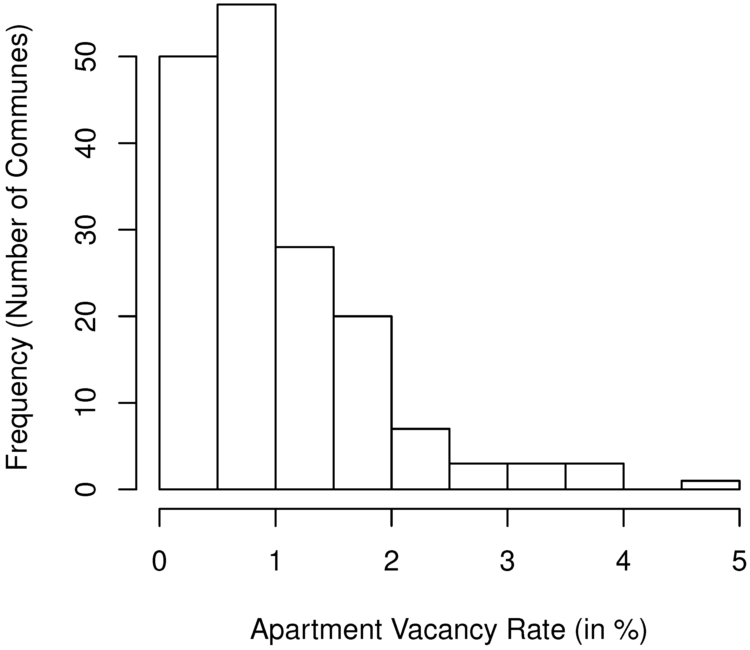
for every lot of land. We refer to this equality as best land use with binding regulation. The assumption that the is binding is reasonable in an urban area with a relative shortage in supply of residential floor space as well as negative externalities arising from high urban density. (Rental apartments exclude owner-occupied apartments by definition. For this reason, the owners of rental apartments are real estate investors who own apartments for investment purposes. Typically, these kinds of real estate holders exploit land efficiently, i.e., fulfill the best land use concept. A debate related to the topic of this paper is the valuation of land under the best use assumption, originally initiated by Smith [3] and his rent gap theory. We refer interested readers to Hammel [38] for a detailed discussion of the rent gap theory and its criticisms. The most important aspect for this study is that the number of apartments built on a land lot is closely related to the best use assumption.) The reason is that the presence of positive externalities and, thus, under a non-binding , the real estate developer would simply build more floor space as long as the marginal profit is positive, i.e., if the costs associated with the physical structure are less than the expected rent revenue. (This model assumption is confirmed by Cai et al. [2] who show that land developer’s housing construction is largely bound by regulations in major Chinese cities. The authors highlight the a highly restrictive constraint as it often lies below the optimal for developers.) In the canton of Zurich, the study area of this paper, the very low vacancy rate of 0.61% for apartments is a strong indicator of a shortage in supply of residential floor space. (The apartment vacancy rate of 0.61% is the average in the canton of Zurich. However, the assumption that the is generally binding requires a shortage in residential floor area in the entire region. Figure A2 in the Appendix A illustrates that this is indeed the case.) In addition, with the constant costs of physical structure, a non-binding would lead to a situation with equal marginal rent prices associated with the location (location rent). However, the empirical section will show that location rents largely vary.
In case of an apartment builder, it follows that an additional m of living area requires of building land. The land use efficiency assumption implies that this relationship is always fulfilled, i.e., no land is wasted and the maximum restriction is not violated. Thus, in order to build an apartment with floor area X (size), the builder requires total land area . In a competitive developers’ market, the assumption of best land use with binding regulation is plausible. (Wheaton [37] argues that local rent maximization is not necessarily the aggregate rent maximization.)
3.2. Local Amenities
The price of an apartment can be attributed to two kinds of amenities: physical attributes and local amenities. Locational attributes are by definition bound to the physical location of an apartment. Local amenities include, for instance, local taxation advantages, the household’s relevant school districts, proximity to goods and services, as well as transport connections. While the physical structure could basically be a standardized unit, the location of the house or the apartment is always unique. From the household’s perspective, the location of the land does not have a physical extent. In particular, amenities, provided externally in the form of public goods and associated with a particular location, are available independent of the size of the land. However, buying more land crowds out other potential bidders for the same location. It follows that the price of the location must somehow depend on the location quantity, i.e., the size of the land, which constitutes the location. As a consequence, the price of the location depends on the lot size. Thus, the rental price must include a location value that depends on the size of the lot of land. (A particular lot of land does not only constitute location. It is associated with two major physical characteristics. On the one hand, the size of the lot restricts the ground floor of the structure. If a structure has only one floor, the land size is a direct restriction of apartment size. On the other hand, the allowed floor-level of a piece of land has physical as well as location characteristics. Living on a higher floor increases the view but also the route from the building entrance to the apartment. However, these property characteristics are neglected in our study. We restrict the analysis on the size of the apartment and the land size necessary to provide this apartment size.)
The competitiveness of locations originates in the land market. We demonstrate how the value of amenities and, thus, the location attractiveness is reflected in the land price. Our model is based on and inherits its conceptual ideas from Parsons [1]. Consider a real estate developer who owns a parcel of land with total area . The land exhibits constant local amenities. The developer can divide the land into m lots of equal size. The local amenities associated with living on a lot of the developer are denoted by A. There is a construction firm from which the developer can build structure with the floor area X (size) at the cost of . The developer can rent out each of the m composite bundles (consisting of structure and land) for a rent . In this setting, the developer faces the following profit maximization problem:
Assume there exists an equilibrium characterized by a bundle with , where is the equilibrium level of location-related attributes and the equilibrium structure attribute. Therefore, the rent in equilibrium is . The number of equally sized land lots follows directly from .
Suppose there is a potential renter who wants to rent an apartment on a lot of land which is a multiple () of the standard lot size. In addition, he/she prefers a specific amount of floor area . The builder would only sell the bundle if: We do not include the value of an option to redevelop in this condition as we assume the best land use within a binding regulation. In the latter hedonic estimation of the total apartment rental price, this assumption contradicts the findings of Clapp and Salavei [39].
We assume that the cost and rent functions are linear. Therefore, the condition for a developer to sell a bundle can be simplified to
Under market competition, this simplification must hold with equality and corresponds to the rental price of the bundle with the large lot size. The price of the bundle with the standard lot size () is .
3.3. The Threefold Nature of Apartment Size
Without a loss of generality, we can set to unit size (one m, for instance). Then, is the lot size in m. By rearranging the pricing equation, the general rental price function is written as
This corresponds to the result derived by Parsons [1], who suggests pricing the location attractiveness by weighting local amenities by lot size. We now include the best land use under a binding regulation, represented by Equation (2), which states that the best use lot size is . The term is the rent for a unit size location. As we have set the unit size to one , we can replace by , denoting the per m land rent.
Furthermore, we assume that the extent of the land only has a positive price if there remains a free and undeveloped space, which, for example, may be used as a garden. This free space is the total land size minus the land occupied by the building. In our setting, the total land size is and the built land can be expressed as , where is the number of levels of the building. The resulting free space can be simplified to . Using this concept of free space, we replace the corresponding price by , where F refers to free space. Therefore, the apartment rent can be written as
By taking the first derivative, the marginal effect of an additional m in apartment size on apartment rent can be determined. This derivative is given as
It follows that the marginal rent of an additional unit in apartment size is composed of three components. The first term is the price for an additional square meter of structure , which is regarded as a globally constant structure price. The second term is the rent price for free land . (The ratio represents a relative weighting for the rent of free space. In case of a constant , this ratio increases in the number of floors. In contrast, in case of a constant number of floors, this ratio declines with an increasing .) Similarly to the structure rent, the value of this component is independent of the location. Finally, the third term in Equation (8) is the rental price for the local amenities per land unit . The rental price therefore consists of prices for two kinds of amenities: physical amenities associated with the free space and amenities associated with the location. Only the last term is directly associated with and, therefore, dependent on the apartment’s location. In this study, we are interested in the land rent for a set of locations.
These locations may be part of urban, sub-urban, or rural areas. Our novel approach has the highest relevance for urban and sub-urban areas where land transactions are scarce. Rural areas tend to be regions with a higher share of homeowners who maximize the quality of life and not the . Therefore, fewer negative externalities arise and our instrumentation of the might not perform as well. In addition, in rural areas land supply is more elastic. Consequently, our approach is not so relevant in rural areas or in areas with high home ownership. (On the contrary, land prices for owner-occupied apartments in metropolitan areas might be derived by using imputed rents in our novel approach. However, this extension might be covered by future research.)
3.4. The Effect of Regulatory Changes on FAR
In order to determine local land values, Equation (7) is estimated based on a hedonic regression model. To provide further interpretation of our theoretical results, we briefly outline the relationship between our exogenous and endogenous variables. Considering the third term in Equation (8) and assuming the floor area of an apartment , the total location price per dwelling is
Depending on the temporal scope, we expect different and ambiguous effects. First, consider a rapid and substantial increase in the in the whole urban area due to a regulatory change. This would increase the supply of floor area and decrease the corresponding rent temporarily. From this perspective, land prices are exogenous, while location prices of dwellings are endogenous. However, the change in the floor area rent will be capitalized into the equilibrium land value. It follows that rental prices are exogenous to the land values in the long run. This non-dynamic equilibrium can be analyzed cross-sectionally. In the empirical section, we estimate land rents using a global hedonic function with time dummy variables, i.e., a quasi-cross-sectional specification with estimated land rents representing average values for a region. Given a particular homogeneous region, the long-term demand for residential floor area is assumed to be highly elastic and therefore constant. With an endogenous land price, it is convenient to rewrite Equation (9) as
by augmenting the with a negative externality parameter . As a change in the directly capitalizes into land values, the parameter is the elasticity of the land price with respect to : (Brueckner et al. [6] interpret this elasticity as a measure of the regulation stringency, namely, the extent to which building decisions diverge from free market outcomes.)
For instance, let us consider two land lots of identical size and identical local amenities, e.g., due to their proximity. However, lot A has a twice as big than lot B. In the absence of negative externalities, the value of lot A would be double the value of lot B. In the case with negative externalities, however, lot A would be less than double the value of lot B as the has a decreasing marginal effect. Formally, we model this expected non-proportionality as , with .
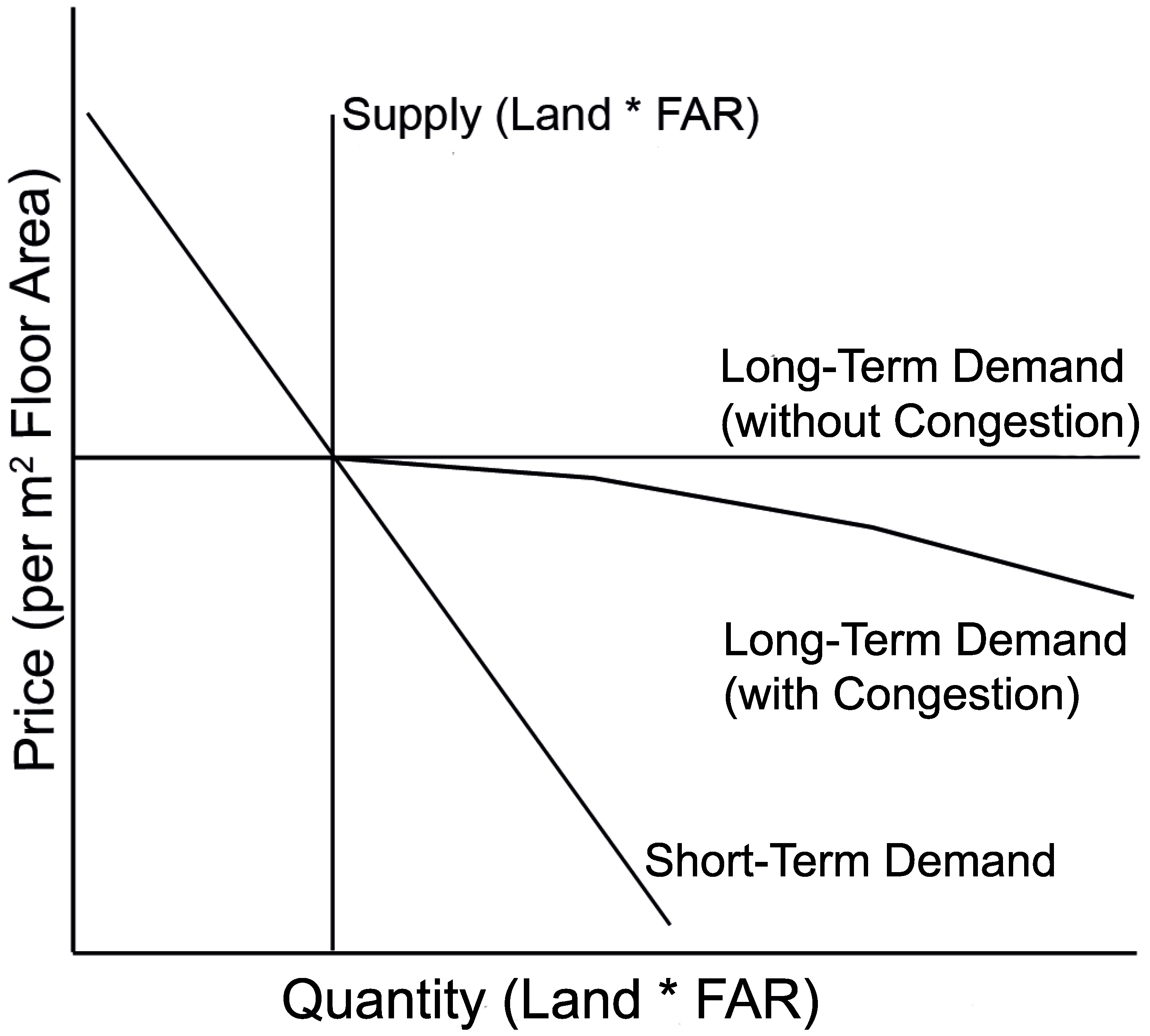
The theoretical considerations about supply of and demand for floor area are illustrated in Figure 1. The best use assumption implies that the supply of floor area on a confined land lot is fixed by the . Therefore, the supply of floor area is perfectly inelastic, unless the regulation changes. The demand of floor area in the short run is inelastic, represented by a downward-sloping demand curve. The long-term demand, however, is highly elastic (due to the presence of alternative locations) and is represented by a horizontal line. An increase in the supply of floor area (by increasing the ) is not supposed to change the price of floor area in the long run. With negative externalities, however, the higher density affects the demand for the local residential floor area in a negative way, which is illustrated as a decreasing long-term demand function.
4. Empirical Results
4.1. Estimation Strategy
In Section 3.2, we demonstrate that the value of land has a physical and location-related component. Assume the residential area is partitioned into subareas with . The subareas are constituted by homogeneous local amenities, i.e., apartments exhibit the same local amenities within a subarea. Therefore, the resulting hedonic equation is
where the total rental price is a sum of the different rent components. First, the price for physical land ( is the rent price for the free space and is the size of the land lot). Second, the price for general physical attributes ( is a vector containing general physical attributes that excludes apartment size and denotes a vector of corresponding rent prices). Third, the price for the physical apartment size and, last, the rental price for location k which is described by . is an indicator function mapping locations to aggregated regions. (The aggregation of single locations is necessary as land transaction price data is only available on a regional level.) The location is defined by the geographical coordinates of the apartment. denotes the error term.
In terms of rental market heterogeneity, this model states that there is only spatial heterogeneity in location prices. Spatial heterogeneity in hedonic pricing models has at least two different aspects. First, the heterogeneous structure of residuals leads to inconsistent estimates of pricing coefficients (see, e.g., Füss and Koller [40]). Second, the residuals can be regarded as the price of unobserved property factors. With our model specification, we account for the spatial heterogeneity by finding a homogeneous area. However, it does not necessarily ensure consistent estimates of the hedonic pricing equation, but rather allows estimating the location values, which determine implicit land prices. Moreover, Glaeser et al. [16] highlight another specification error. Similar to their findings, a bias may arise if the total living area is correlated with omitted apartment characteristics which we cannot specifically control for. For example, if bigger apartments tend to be in areas of higher quality, the omitted characteristic will increase the coefficient and vice versa.
In order to estimate location prices, we need to differentiate between the physical and the locational land value. This is achieved by including the interaction of homogeneous areas with land size:
where denotes an indicator variable reflecting whether apartment i is located in area k. The coefficients , are the estimates for regional land rents, our parameters of interest. Note that the superscript r in indicates that the estimation coefficients are relative rents as the intercept of the land rents cannot be identified from the interaction with region dummies. Therefore, the model explains the spatial variation rather than the absolute level of land rents. The absolute land rent is therefore . This relationship is discussed in the next section.
Principally, conclusions about the goodness-of-fit of the model can be drawn by comparing the predicted land values with actual transaction prices. However, it is also common to compare the goodness-of-fit with a benchmark model. Because in hedonic pricing models locational variation is often captured by location dummies, the location dummy model serves as our benchmark model. Formally, it can be written as
In the case of this dummy model, the parameter cannot be interpreted as a land rent per m. However, the location dummies have the potential to capture the variation in locational values.
4.2. Transformation of Land Rents into Land Values
In this section, we demonstrate how absolute land values can be estimated from relative, regional land rents . Obviously, this transformation must include a shift in levels (because rental prices are determined in relative terms) as well as a capitalization rule, which transforms land rents into land prices. In order to keep the model tractable, we assume that a single (and constant) land capitalization rate d exists for all regions. Thus, the required transformation can be formulated as
where is the level coefficient to transform the relative into an absolute rent and d is the capitalization rate for the land value. Therefore, the term refers to the level factor which transforms the relative land price into the absolute land price. One possible approach is to make assumptions about and d, as well as about land price predictions. However, we use observed regional land price data to estimate these coefficients in order to test the validity of our implicit land price model. While model testing is the main purpose of our estimation strategy, we additionally derive an estimate for this land capitalization rate.
In appraisal-based valuation, the overall capitalization rate is defined as the value-weighted average of a building (structure) as well as a land capitalization rate [7]. Therefore, our land capitalization rate only reflects the risk linked to the location and neglects risks associated with the structure. In addition, our land capitalization rate is given in gross terms. However, the difference to the net capitalization rate is small as other income, vacancy losses, and operating expenses on a land lot are of small magnitude and, thus, negligible.
4.3. Data and Study Area
Our empirical analysis uses an extensive data set for the canton of Zurich, Switzerland, which is an ideal study area as the canton’s land use regulation is subsidiary to a national land use plan. The building law in Zurich allows for a wide range of measures to “establish a foundation for human development”. (Written in Planungs- und Baugesetz [planning and building law], §18, Abs.1.) This variety of instruments makes the consideration of individual regulatory measures impossible. Therefore, we restrict our attention to the most important, and for our analysis sufficiently adequate, regulatory measure: the , which is defined as the maximal total floor area divided by total lot area . (Defined in the Planungs- und Baugesetz [planning and building law], §254 and in more detail in the Bauordnung der Stadt Zürich 2012 [building regulation of the city of Zürich 2012].) Most importantly, the regulatory setting in the canton of Zurich allows us to assume that the land use regulation is likely to be binding. The canton comprises urban, suburban, and rural areas (depicted in Figure A1). In urban areas, for example, in the city center of Zurich, the is certainly binding as a the high demand for space would make it profitable to develop residential buildings in a denser way. However, observed residential buildings show similar density restrictions (number of floors, garden size, etc.) which validates the restrictiveness of the . The same argumentation holds in suburban regions where the is lower. However, only in rural neighborhoods development of residential buildings might not fully exploit the in some cases due to the lower demand for space. The variation of the FAR in the canton of Zurich is shown in Figure 5.
The first data source for our dataset is the parcel data record provided by the statistical office of the canton of Zurich. This geographic information system (GIS) data contain the location and shape of all land parcels in the canton of Zurich as well as the corresponding building rights and regulations (including the ). By using the coordinates of the rental data, the apartment’s underlying land as well as its building rights can be determined. This rental price data stems from our second data source: a multiple listings service. Overall, our data contain more than 49,501 observations from 2002 to 2014 including a wide set of apartment characteristics for the categories rental price, structure, location, and time, as shown in Table A1 in the Appendix A. The apartments come with a street address, which enables us to find coordinates using a geocoding service. (We use Google’s geocoding API to translate street addresses into global coordinates. These coordinates are then transformed into Swiss Grid coordinates by a transformation function provided by Swisstopo.) Using this rental data has the advantage that the number of observations is large, as rental dwellings change hands more often and an overwhelming majority of households in Zurich are renters. Property and vacant land transactions are sparse in the Zurich urban area and the share of owner-occupiers, for both houses and apartments, only lies around 7% in the central city. This makes the canton of Zurich an excellent laboratory for our study.
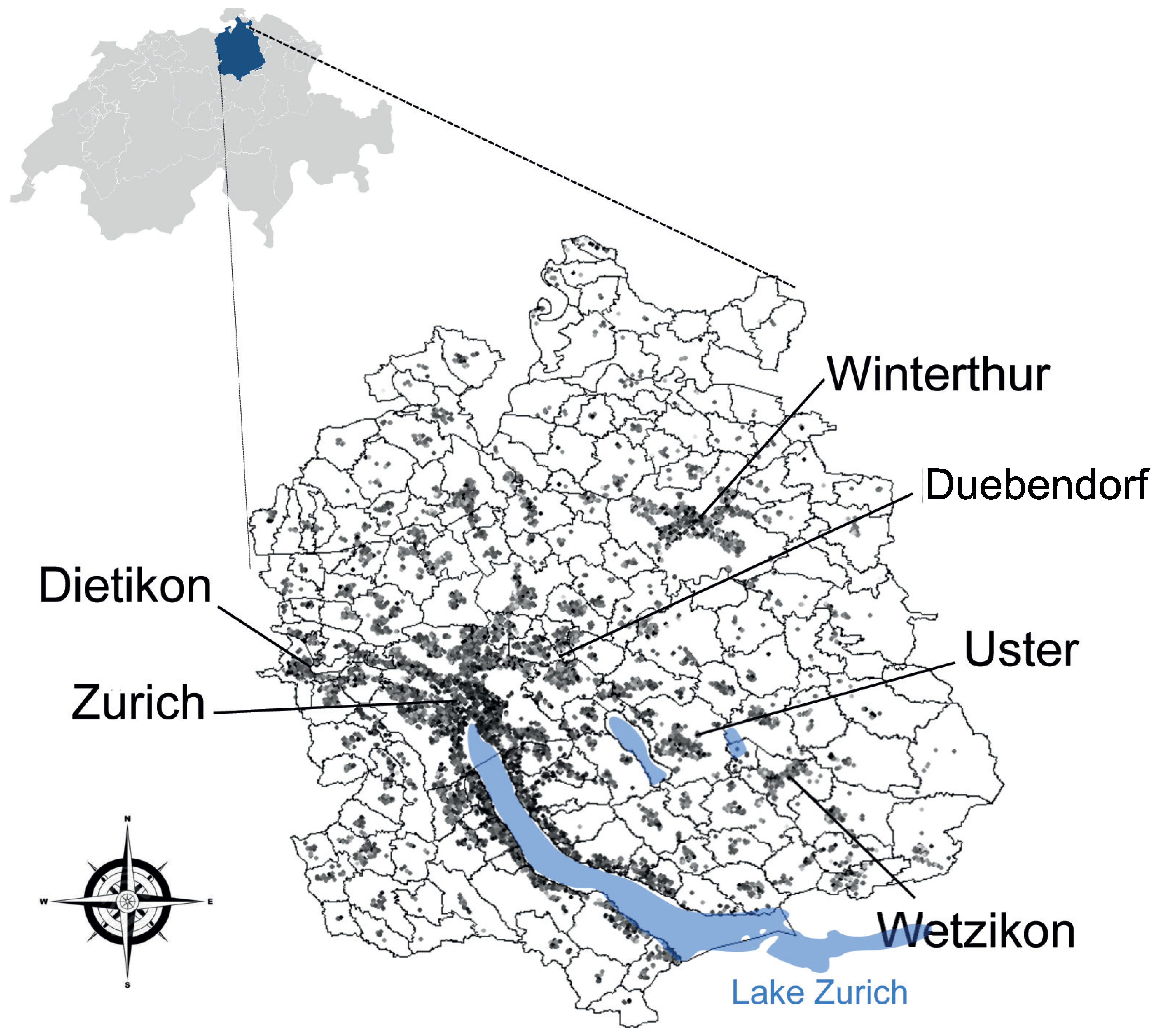
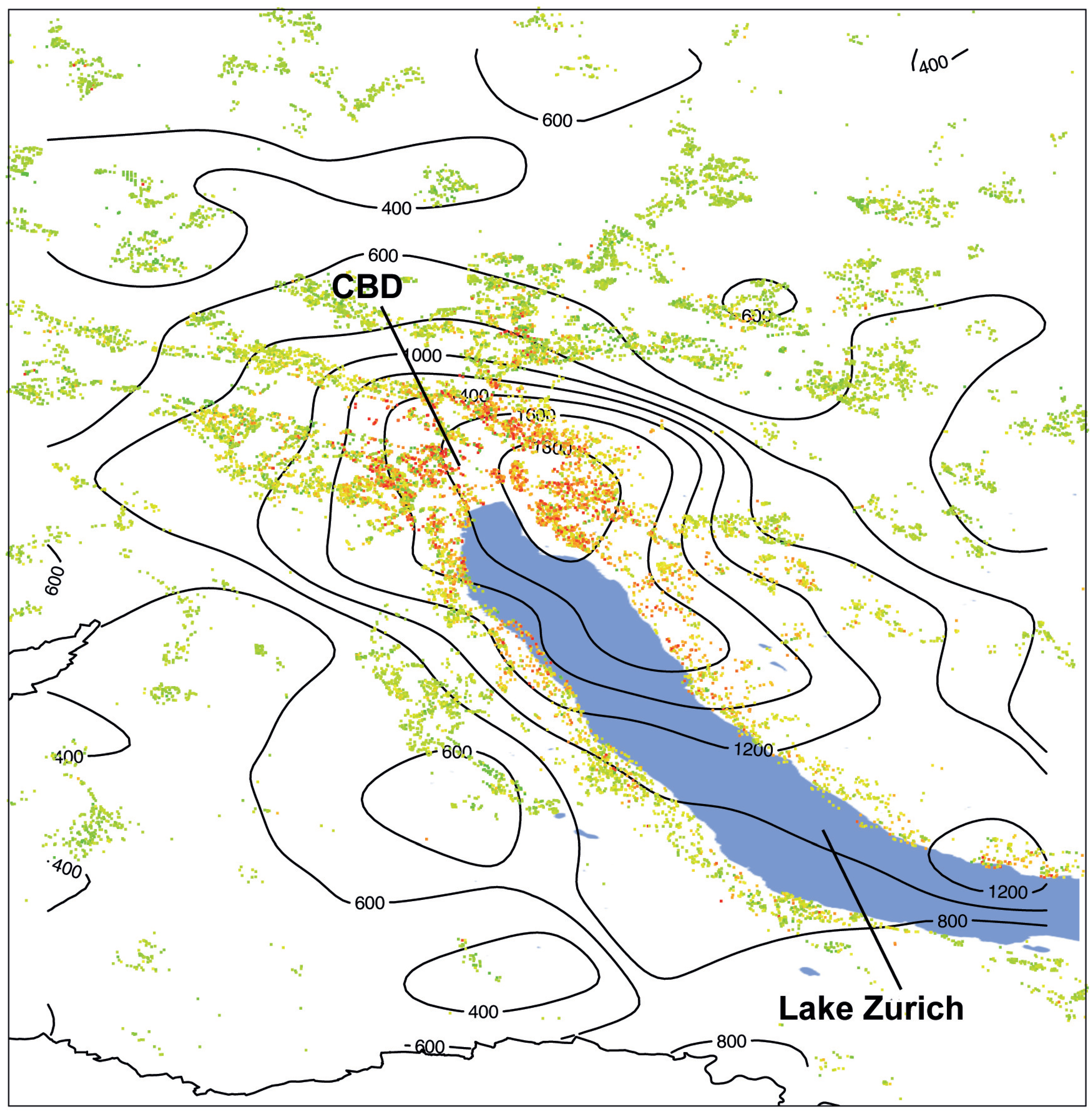
Figure 2 shows a map of the canton of Zurich with the spatial dispersion of rental observations represented by the dots, where light and dark colors represent low and high rents, respectively. The smallest jurisdictions are 171 communes, illustrated by solid shapes and listed in Table A2 in the Appendix A. The largest city in the canton is Zurich City, with a population of 383,708 at the end of 2013. The second largest city is Winterthur. In terms of population (105,461), Winterthur is only about one-quarter of the size of Zurich City. The population in these two cities accounted for almost 35% of the canton’s total population (1,421,895) at the end of 2013. In our data, 36% of the observations stem from Zurich and Winterthur, i.e., the data represent the dispersion of residents. Moreover, comparing the data to BFS’s 2012 nationwide household survey shows that the rent prices of the apartments have representative mean values. For instance, in the canton of Zurich, the average rent price of an apartment with three rooms was 1442 CHF, and 2354 CHF for an apartment with four rooms. (The corresponding average rent prices in the BFS nationwide household survey were 1419 and 2137 CHF. See Strukturerhebung [41] for more information.)
The Zurich Statistical Office provides our third data source on regional averages of land price transactions. The corresponding data is based on communal land registry offices, where all property transactions must be registered. For confidentiality reasons, only averages of these transaction prices are reported. (See Statistisches Amt des Kantons Zürich [42].)
4.4. Testing the Model
In Section 3, we outline theoretically how the relative rental price is transformed into absolute land prices. Now, we make use of regional land prices to empirically test the model in two steps. In the first step, we estimate the model of relative implicit land rents, , according to Equation (13). In the second step, these estimates are compared to observed regional land prices as suggested in Equation (15). To derive the level coefficient and the land capitalization rate d, we run a regression of regional (aggregated) average land prices on our implicit relative land rents for the corresponding regions. (As we assume homogenous construction costs in the canton of Zurich, we refrain from modeling the construction sector explicitly. This assumption seems valid due to the perfect competition of construction companies within in the canton and the strong regulations that only allow foreign competitors to enter the market at the same labor costs as well as material expenses.)
As mentioned above, the sparsity of vacant land transactions is one of the main reasons for the use of residential data to determine land values. For the same reason, however, we use averages of regional land transaction prices to test the predictive power of our model. A higher level of aggregation (i.e., larger regions) of land transaction prices has the advantage of increasing the sample and therefore improving the accuracy of mean land price estimates. The disadvantage is, however, that fewer (aggregated) observations are available to test its predictive power. This trade-off is restricted by the availability of data. We have access to regional mean prices for two regional aggregation levels: 171 communes and 12 consensus land use planning regions. On the level of communes, the number of land transactions ranges from 0 to 26, with an average of 2.6 transactions per commune and year. On the level of consensus land use planning regions, the corresponding range is from 16 to 72, with an average of 40.5 transactions. As we do not have observations for each commune in every year, the communal aggregation level of land price transactions is not suitable. For this reason, we decide to use the predefined consensus land use planning regions to test the predictive power of the model.
Although the time dimension is not of prior interest in our analysis, we include yearly time dummies to account for temporal effects. The regression results of the first step are listed in Table 1. Besides the hedonic rental prices for different apartment characteristics, the coefficients represent the implicit relative land rents for regions 1 to K.
To illustrate the meaning of the coefficients in the first step regression results, we choose two apartments from different regions. The first apartment is located in the central city of Zurich (region ID = 261). The annual rent for the apartment is 40,200 CHF. The floor area is 85 m and the on the land lot is 130%. The minimum required land size (efficient land size) to supply this floor area is 85 mm. The estimated coefficient of the efficient land size in region 261, i.e., the relative land rent, is = 69.6 CHF. It follows that the incremental rent of the apartment, associated with the required land, amounts to = 4551.8 CHF per year. The second apartment is located in a smaller town called Uster (region ID = 198). The annual rent of the apartment is 20,200 CHF. With a floor area of 94 m and of 65%, the efficient land size is 94 m = 144.6 m. Given the relative land rent = −2.07 CHF, the incremental rent of the second apartment, associated with the required land, is = −299.3 CHF per year.
We can now calculate the difference of the relative land rents of the two apartments, which amounts to 4551.8 CHF − (−299.3 CHF) = 4851.1 CHF. Therefore, we estimate that the rent associated with the land of the first apartment is 4851.1 CHF higher than the rent of the second apartment. In other words, the 4851.1 CHF of the rent difference can be explained by differences in the attractiveness of the location combined with the difference in the required land consumption. In contrast to relative land rents, the coefficients of the physical characteristics (hedonics) are estimated globally, i.e., without a location interaction. For instance, the estimated annual price for a m of floor area is 174.9 CHF. Furthermore, an important result of the estimation is that the coefficient of the efficient land size is very small. This means that the rent associated with the free land is economically negligible for the rental apartments in our data set.
In the second step, we compare the implicit relative land prices to the observed absolute mean land prices of the planning regions. Figure 3 shows the scatter plot of the two variables. This graph indicates a strong linear dependence that is also reflected in a high correlation coefficient of 0.936 between actual and predicted land values.
Moreover, the results of the linear regression in Equation (15) of (aggregated) effective land prices on implicit land rents are summarized in Table 2. Columns (1–4) are based on the results of the interaction model, specified in Equation (13). More specifically, in columns (1–3), we perform the analysis for different sub-periods as a robustness test of the main results for the whole sample period, which are given in column (4). In the respective columns, the land capitalization rate for each sub-sample is given as well, which allows identifying its temporal development. Column (5) uses the regression results of the location dummy model, specified in Equation (14), which serves as a benchmark for our baseline estimation.
For the whole time period, we conclude that our prediction of land price data is accurate. The high on an aggregate level suggests high accuracy of the land prediction model. The result does not only provide supporting evidence for our theoretical model, but also makes it feasible for practical applications. In other words, it shows how differences in local amenities finally capitalize into land prices. In addition, the analysis of different sub-periods indicates that these results remain robust over time.
Further, the comparison of land price predictions with the location dummy model shows a favorable result for the interaction model. As the of the two models indicates, the goodness-of-fit of the interaction model is higher, and thus outperforms the benchmark model. However, the difference in the is relatively small, which most likely can be traced back to the aggregation effect since predictions are tested against aggregated land prices of planning regions. On this level of aggregation, the variation of the is likely to be averaged out to some degree. Nevertheless, the goodness-of-fit is higher for the interaction approach.
As a by-product of the goodness-of-fit test, we report the level and slope coefficients in Table 2. The slope estimate of 13.110 corresponds to the inverse of the land capitalization rate. For the whole sample period, the capitalization rate for the land value is therefore 1/13.110 = 7.63%, which is relatively high compared to discount rates of real estate development projects and may be biased due to the previously mentioned specification error [16]. Moreover, as mentioned earlier, this land capitalization rate is in gross terms, i.e., the rent related to a land lot excludes the costs associated with the provision of a dwelling. In addition, as our analysis is restricted to the location value (rather than the value of physical characteristics), the land capitalization rate corresponds to the location rent and location price, respectively. Presuming that the risk associated with the location of the real estate is higher than that associated with its structure, a higher rate is not surprising. Concerning the temporal development, the land capitalization rate strongly decreased from 2002 to 2014, with a land capitalization rate of 5.68% for the recent sub-period 2010–2014. This finding is in line with a decreasing interest rate over the same time period. (As mentioned in the previous section, the coefficients of the location dummy model are not location rents. Therefore, the slope coefficient cannot be interpreted as capitalization rate.) The estimation of the level coefficient and the land capitalization rate d allows us to identify a further parameter: the global negative externality parameter . The parameter is obtained by maximizing the goodness-of-fit in the second step regression:
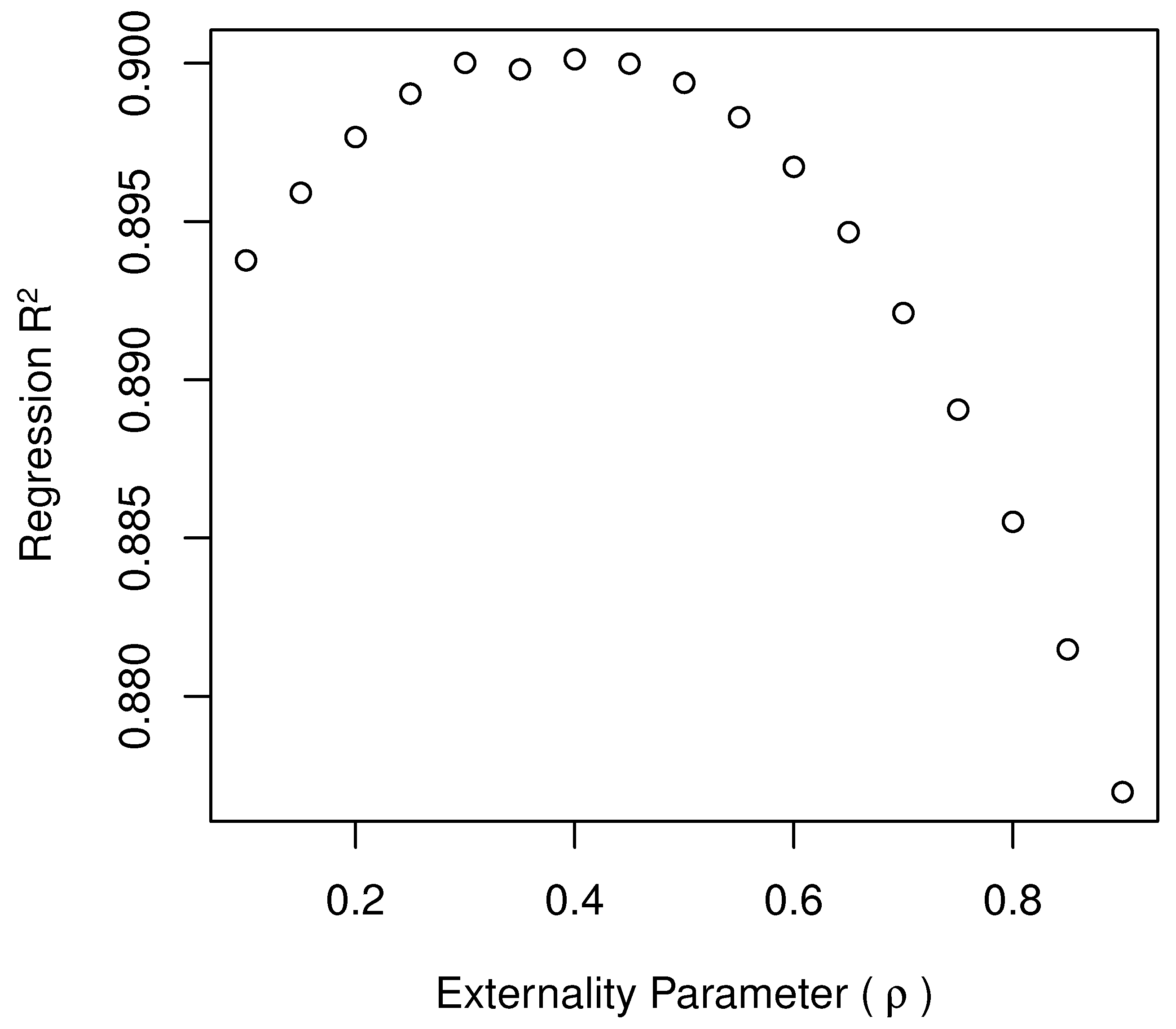
We estimate a value of , which means that the is associated with negative externalities. The goodness-of-fit of the second step regression (in terms of ) is shown in Figure A3 in the Appendix A. A negative externality parameter of implies a diminishing effect of the on land prices, e.g., the effect of a of 2 on land prices is or .
4.5. Land Value Surface
In the previous section, we have shown that the implicit land price model is able to fit land price transaction data accurately. As a by-product of this test, we estimated coefficients that allow us to predict land prices from implicit land rents. Based on these results, we are able to estimate a land value surface by smoothing the predicted (implicit) land values. For this purpose, we spatially generalize the rent function in Equation (12) to receive (We follow the notations of Clapp and Wang [43] for the specification of the hedonic pricing model.)
In particular, we run a nonparametric local regression of land price predictions (at individual level) on Swiss Grid coordinates. Therefore, we follow the classic literature regarding the use of local regression models to develop land price surfaces including those in [44,45] (Originally, these methods are proposed for local linear regressions in [46], and are first applied to land valuation in [47].) by the model specification is based on the Nadaraya–Watson local constant estimator:
where
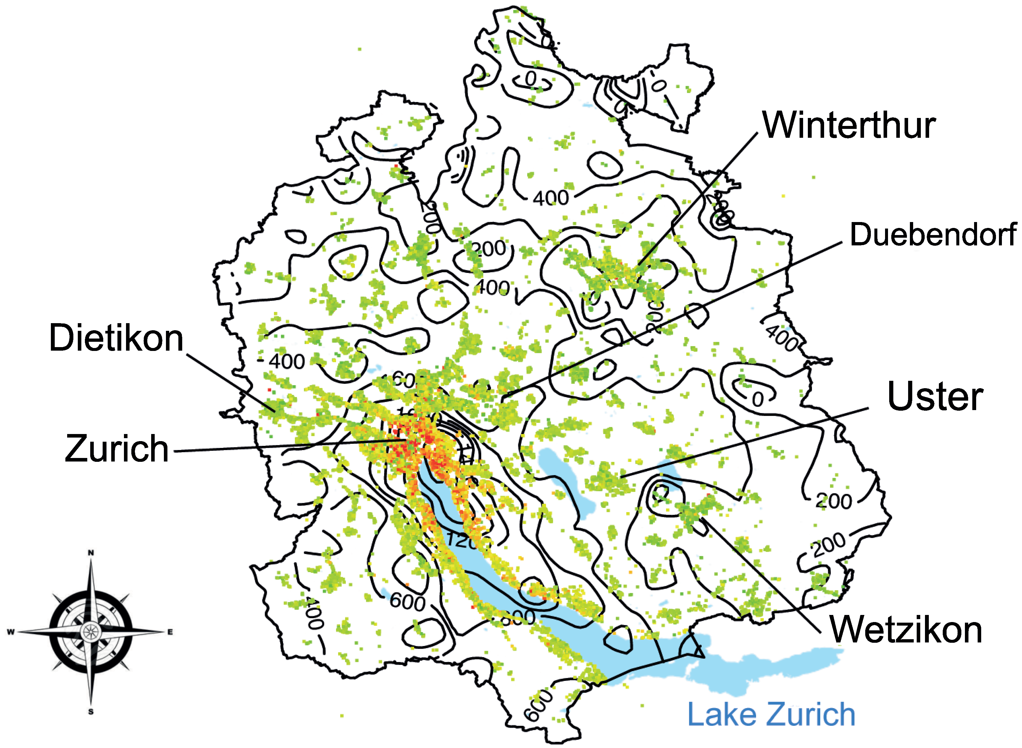
We use a Gaussian Kernel function with a bandwidth h, which is determined by an unbiased least-squares cross-validation. As a result, we get a smooth surface of relative residential rents. Based on Equation (15), these estimates are transformed into land value estimates. The corresponding smooth land value surface is depicted in Figure 4.
The predicted land prices in the canton of Zurich obtain a monocentric structure around the center of Zurich City. The gradient does not have the same magnitude in every direction. Particularly, the slope of gradient is significantly lower alongside the lake. Besides the city of Zurich, different local elevations in land prices can be identified around the city of Winterthur.
In the next step, we need to highlight how the predicted land values of the canton of Zurich can be explained by major land attributes. First, note that the land price surface smooths out the micro-location to some degree. Therefore, it is primarily associated with macro-location values. Our findings are largely in line with Kubli et al. [48] and confirm that the macro-location is indeed the most important determinant of land prices in this area. The corresponding land attributes are distance to CBD, tax level, and proximity to the lake. Because proximity to the lake is a matter of the larger environmental situation, we classify it as a macro-location attribute as well. A closer look to the city of Zurich in Figure 4 illustrates the multi-radial monocentric land prices in more detail. The center is located next to the lake, very close to the CBD. As the contour lines indicate, land prices along the lakeside decrease much slower compared to all other directions.
4.6. Dual Monocentric Structure
From a theoretical perspective, we have argued that the best use lot size is a promising measure for determining land values and we have shown empirically that the predicted land values fit the actual data well. In particular, interacting the best use lot size with local amenities is successful for land price determination. In this section, we restrict the analysis to the metropolitan region of Zurich to demonstrate the monocentric structure of implicit land prices and to illustrate how the role of land use regulation is reflected in this pattern of implicit land prices.
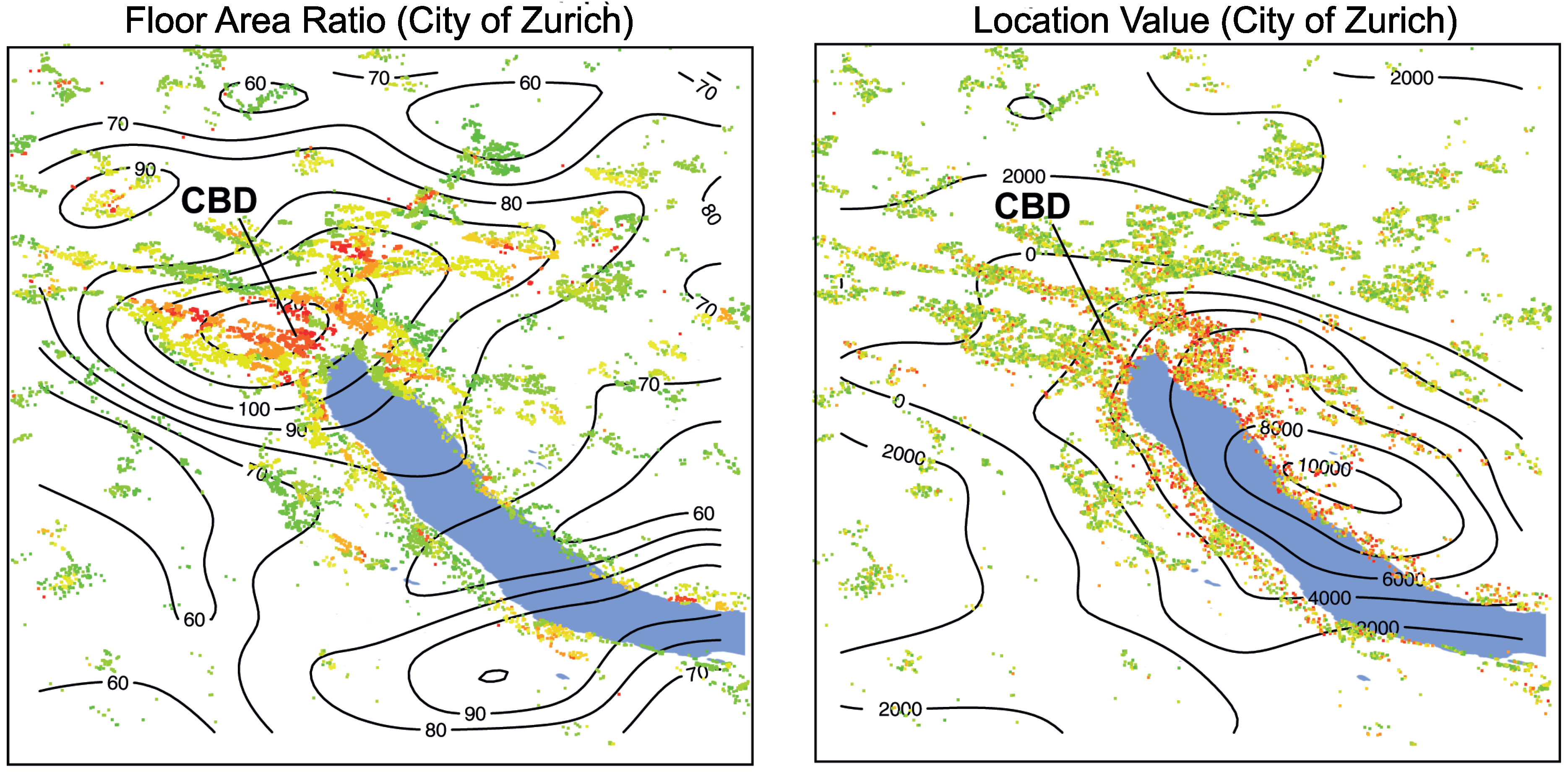
The predicted land value is the product of location value per m and land quality. We can decompose these two factors and analyze them visually. First, we focus on the central location’s attractiveness, which is reflected in the left panel of Figure 5. The graph shows a nonparametric surface of the location value. The CBD has the highest value and location prices are decreasing in all directions. However, the monocentric structure is distorted and irregular, with the lakeside naturally being the main source of irregularity for the location value. In summary, location values exhibit a monocentric structure, even without controlling for non-monocentric location amenities such as proximity to the lake.
Second, the fact that the is higher in central areas increases land rents in the CBD. Due to the correlation between these two location characteristics (location attractiveness and ), the implicit land prices exhibits considerable variation. Indeed, the building regulation aims at a high in central locations, where the location value is already high. The obvious reason for this policy is to reduce prices for dwellings at favorable, central locations.
Finally, the predicted land values as the product of location quality and land quality are shown in Figure 6. The interaction of location value and location quality is embodied in this surface. The monocentric structure of land quality has clearly shaped the land price patterns into oval gradients. However, the pattern of the location values dominates the high value locations along the lakeside. In addition, the location value determines the center of the monocentric structure in land prices. Indeed, the highest land price is not in the CBD, but slightly more northward next to the lake. In this area, very high local amenities meet a relatively high , making this location the most valuable land in the canton of Zurich.
5. Conclusions
In this paper, we show that under binding land use regulation, the per m price of land is a direct function of the local amenities and the restrictiveness of regulations. Thereby, we use the , a very common regulatory instrument for urban density in the study area, to formulate a simple model that emphasizes the best land use assumption, i.e., the optimal exploitation of the land under regulation. In the model, we show that an additional unit of apartment surface requires units of land. Moreover, for a constant , it can be proven that the marginal price for the apartment size has three rent components: the presumably constant rents for structure and physical land, as well as the land-rent inherent location value.
In the case of binding , the interaction of locations with lot size under best use is a promising approach to determine land price variations from land rents. Therefore, we formulate a theoretical model in which the potential apartment rent is capitalized into land values. We then show empirically how to use apartment rent data to determine per m land prices by applying the model to a hedonic setting based on an extensive sample of rental data in the canton of Zurich. This linear transformation of rent components into land prices estimates the land capitalization rate as a coefficient as well.
We demonstrate that our model is highly reliable in predicting land prices. In particular, the correlation coefficient between predicted values and observed land prices is 0.936, and the relative prediction error is 18.9%. This high prediction accuracy makes the model suitable for practical application. For instance, it provides a basis for predicting land values at locations where land transactions are infrequent or even absent. This is particularly helpful as land transactions tend to be low in urban areas, where rent observations are very frequent. Moreover, the comparison of the model with a benchmark (location dummy model) demonstrates its superiority in explaining spatial land prices.
As a by-product of the goodness-of-fit test of our model, we estimate a land capitalization rate of 7.63%. This finding is interesting from an asset pricing perspective. Particularly, it can serve as a benchmark capitalization rate for real estate investments. However, the derived return on investment cannot be compared to capitalization rates used for real estate appraisal purposes, because it is a gross rate and is associated with the land value only.
In a final step, we utilize our findings from the model test to estimate a land value surface. In doing so, the number of observations allows us to use a nonparametric approach to predict land values for any location. Concentrating on the metropolitan region of Zurich, we find a monocentric pattern in the predicted land values. This monocentricity is the result of two main sources affecting the urban spatial structure: First, the monocentric location value pattern is the result of higher amenities in central locations. Second, the monocentric land quality pattern is the result of land use regulation, i.e., the result of the higher permitted floor area ratios in central areas. Thus, when estimating land values, and especially, when the location values stem from regression residuals, land quality should be accounted for.
Author Contributions
Conceptualization, R.F. and J.A.K.; methodology, R.F. and J.A.K.; formal analysis, J.A.K. and A.W.; resources, R.F., J.A.K. and A.W.; data curation, J.A.K.; writing—original draft preparation, R.F., and J.A.K.; writing—review and editing, R.F., J.A.K. and A.W.; visualization, J.A.K. and A.W.; supervision, R.F.; project administration, R.F., J.A.K. and A.W.; All authors have read and agreed to the published version of the manuscript.
Funding
Not applicable.
Institutional Review Board Statement
Not applicable.
Informed Consent Statement
Not applicable.
Data Availability Statement
The data is not publicly available and cannot be shared due to a non-disclosure agreement.
Acknowledgments
We have benefited from the discussion with Zeno Adams, Martin Brown, Stefan Fahrländer, Pascal Gantenbein, Kyle Mangum, Anders Österling, Daniel Ruf and to those who participated in the European Real Estate Society (ERES) 2016 conference, the 2017 Swiss Real Estate Research Congress, the 45th American Real Estate and Urban Economics Association (AREUEA) National Conference, as well as the doctoral seminar at the University of St.Gallen (HSG).
Conflicts of Interest
The authors declare no conflict of interest.
Appendix A

Table A1.
Data description. (This table lists the apartment characteristics of rental dwellings by category, i.e., by rental price, structure, location, and time. The data set contains 49,501 observations provided by a multiple listing service for apartment offerings in the canton of Zurich from 2002 to 2014.)
| Category | Variable | Description |
|---|---|---|
| Rental price | Rental price | Gross rental price in Swiss Francs per month |
| Structure | Area | Living area of the apartment in m |
| Rooms | Number of rooms. Living rooms counting for 1.5 rooms | |
| Special view | Binary variable, indicating whether the apartment has special view | |
| Lift | Binary variable, indicating whether the apartment has a lift | |
| Parking | Binary variable, indicating whether the apartment | |
| offers a parking opportunity | ||
| Garage | Binary variable, indicating whether the apartment | |
| has a parking garage space | ||
| Standard | Binary variable, indicating whether it is a standard apartment | |
| Duplex | Binary variable, indicating whether it is a duplex apartment | |
| Attic | Binary variable, indicating whether it is a penthouse apartment | |
| Roof | Binary variable, indicating whether it is a roof apartment | |
| Studio | Binary variable, indicating whether it is a studio apartment | |
| OneRoom | Binary variable, indicating whether it is a one room apartment | |
| Furnished | Binary variable, indicating whether the apartment is furnished | |
| Terrace | Binary variable, indicating whether the apartment has a terrace | |
| InHome | Binary variable, indicating whether it is an apartment | |
| within a single-family detached home | ||
| Loft | Binary variable, indicating whether it is a loft apartment | |
| Location | Address | Street address of the apartment |
| Time | Availability | Date of availability of the apartment |
Table A2.
Municipalities in the canton of Zurich. (This table lists all 171 municipalities in the canton of Zurich alphabetically. Moreover, a regional identifier () is linked to each jurisdiction.)
Table A2.
Municipalities in the canton of Zurich. (This table lists all 171 municipalities in the canton of Zurich alphabetically. Moreover, a regional identifier () is linked to each jurisdiction.)
| ID | Name | ID | Name | ID | Name | ID | Name |
|---|---|---|---|---|---|---|---|
| 1 | Aeugst a.A. | 56 | Embrach | 115 | Gossau | 192 | Egg |
| 2 | Affoltern a.A. | 57 | Freienstein-Teufen | 116 | Grueningen | 193 | Faellanden |
| 3 | Bonstetten | 58 | Glattfelden | 117 | Hinwil | 194 | Greifensee |
| 4 | Hausen a.A. | 59 | Hochfelden | 118 | Rueti | 195 | Maur |
| 5 | Hedingen | 60 | Hoeri | 119 | Seegraeben | 196 | Moenchaltorf |
| 6 | Kappel a.A. | 61 | Huentwangen | 120 | Wald | 197 | Schwerzenbach |
| 7 | Knonau | 62 | Kloten | 121 | Wetzikon | 198 | Uster |
| 8 | Maschwanden | 63 | Lufingen | 131 | Adliswil | 199 | Volketswil |
| 9 | Mettmenstetten | 64 | Nuerensdorf | 132 | Hirzel | 200 | Wangen-Bruettisellen |
| 10 | Obfelden | 65 | Oberembrach | 133 | Horgen | 211 | Altikon |
| 11 | Ottenbach | 66 | Opfikon | 134 | Huetten | 212 | Bertschikon |
| 12 | Rifferswil | 67 | Rafz | 135 | Kilchberg | 213 | Bruetten |
| 13 | Stallikon | 68 | Rorbas | 136 | Langnau a.A. | 214 | Daegerlen |
| 14 | Wettswil a.A. | 69 | Wallisellen | 137 | Oberrieden | 215 | Daettlikon |
| 21 | Adlikon | 70 | Wasterkingen | 138 | Richterswil | 216 | Dinhard |
| 22 | Benken | 71 | Wil | 139 | Rueschlikon | 217 | Elgg |
| 23 | Berg a.I. | 72 | Winkel | 140 | Schoenenberg | 218 | Ellikon a.d.Th. |
| 24 | Buch a.I. | 81 | Bachs | 141 | Thalwil | 219 | Elsau |
| 25 | Dachsen | 82 | Boppelsen | 142 | Waedenswil | 220 | Hagenbuch |
| 26 | Dorf | 83 | Buchs | 151 | Erlenbach | 221 | Hettlingen |
| 27 | Feuerthalen | 84 | Daellikon | 152 | Herrliberg | 222 | Hofstetten |
| 28 | Flaach | 85 | Daenikon | 153 | Hombrechtikon | 223 | Neftenbach |
| 29 | Flurlingen | 86 | Dielsdorf | 154 | Kuesnacht | 224 | Pfungen |
| 30 | Andelfingen | 87 | Huettikon | 155 | Maennedorf | 225 | Rickenbach |
| 31 | Henggart | 88 | Neerach | 156 | Meilen | 226 | Schlatt |
| 32 | Humlikon | 89 | Niederglatt | 157 | Oetwil a.S. | 227 | Seuzach |
| 33 | Kleinandelfingen | 90 | Niederhasli | 158 | Staefa | 228 | Turbenthal |
| 34 | Laufen-Uhwiesen | 91 | Niederweningen | 159 | Uetikon a.S. | 229 | Wiesendangen |
| 35 | Marthalen | 92 | Oberglatt | 160 | Zumikon | 230 | Winterthur |
| 36 | Oberstammheim | 93 | Oberweningen | 161 | Zollikon | 231 | Zell |
| 37 | Ossingen | 94 | Otelfingen | 171 | Bauma | 241 | Aesch |
| 38 | Rheinau | 95 | Regensberg | 172 | Fehraltorf | 242 | Birmensdorf |
| 39 | Thalheim a.d.Th. | 96 | Regensdorf | 173 | Hittnau | 243 | Dietikon |
| 40 | Truellikon | 97 | Ruemlang | 174 | Illnau-Effretikon | 244 | Geroldswil |
| 41 | Truttikon | 98 | Schleinikon | 175 | Kyburg | 245 | Oberengstringen |
| 42 | Unterstammheim | 99 | Schoefflisdorf | 176 | Lindau | 246 | Oetwil a.d.L. |
| 43 | Volken | 100 | Stadel | 177 | Pfaeffikon | 247 | Schlieren |
| 44 | Waltalingen | 101 | Steinmaur | 178 | Russikon | 248 | Uitikon |
| 51 | Bachenbuelach | 102 | Weiach | 179 | Sternenberg | 249 | Unterengstringen |
| 52 | Bassersdorf | 111 | Baeretswil | 180 | Weisslingen | 250 | Urdorf |
| 53 | Buelach | 112 | Bubikon | 181 | Wila | 251 | Weiningen |
| 54 | Dietlikon | 113 | Duernten | 182 | Wildberg | 261 | Zurich |
| 55 | Eglisau | 114 | Fischenthal | 191 | Duebendorf |
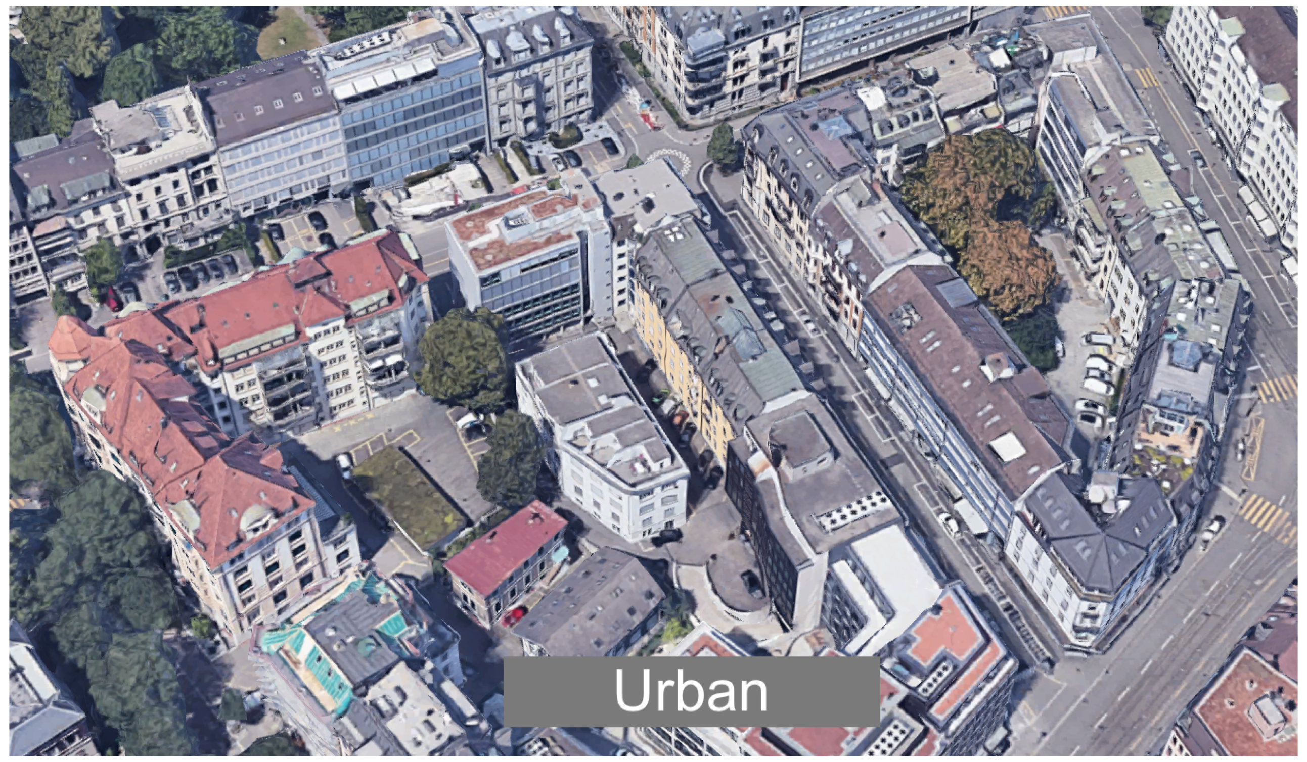
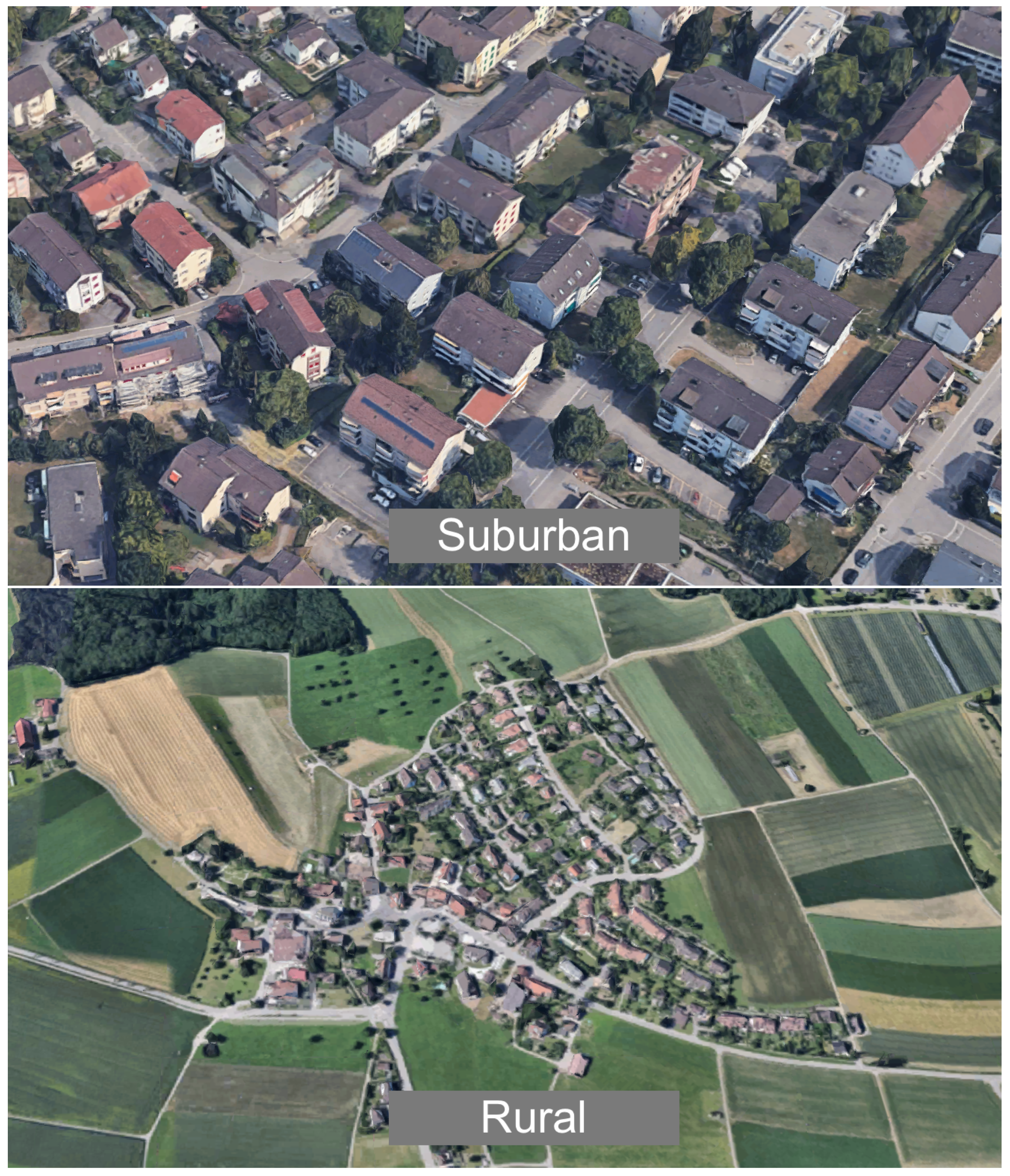
Figure A1.
Urban, suburban, and rural areas in the canton of Zurich. (These illustrations show exemplary neighborhoods in urban, suburban, and rural areas of the canton of Zurich. The urban neighborhood is located at Bleicherweg, Zurich. The suburban area can be found at Talackerstrasse, Opfikon, and the rural neighborhood is located at Neuhofstrasse, Lindau. All pictures are taken from Google Maps/Streetview).


Figure A2.
Apartment vacancy rates. (This figure illustrates the apartment vacancy rate across municipalities in the canton of Zurich. Out of 171 municipalities, more than half have an apartment vacancy rate of less than 1%. Overall, the average is 0.61%).
Figure A2.
Apartment vacancy rates. (This figure illustrates the apartment vacancy rate across municipalities in the canton of Zurich. Out of 171 municipalities, more than half have an apartment vacancy rate of less than 1%. Overall, the average is 0.61%).

Figure A3.
as a function of the negative externality parameter. (This figure illustrates the development of the goodness-of-fit of the overall regression in terms of derived from Equation (15) based on various levels of the global negative externality parameter . With a negative externality parameter of 0.65, the effect of the floor to area ratio () on land prices is decreasing. Therefore, the graph demonstrates negative externalities caused by the ).

References
- Parsons, G. Hedonic Prices and Public Goods: An argument for Weighting Locational Attributes in Hedonic Regressions by Lot Size. J. Urban Econ. 1990, 27, 308–321. [Google Scholar] [CrossRef]
- Cai, H.; Wang, Z.; Zhang, Q. To Build above the Limit? Implementation of Land Use Regulations in Urban China. J. Urban Econ. 2016, 98, 223–233. [Google Scholar] [CrossRef]
- Smith, N. Toward a Theory of Gentrification—A Back to the City Movement by Capital, not People. J. Am. Plan. Assoc. 1979, 45, 538–548. [Google Scholar] [CrossRef]
- Ihlanfeldt, K. The Effect of Land Use Regulation on Housing and Land Prices. J. Urban Econ. 2007, 61, 420–435. [Google Scholar] [CrossRef]
- Kok, N.; Monkkonen, P.; Quigley, J. Land Use Regulations and the Value of Land and Housing: An Intra-Metropolitan Analysis. J. Urban Econ. 2014, 81, 136–148. [Google Scholar] [CrossRef] [Green Version]
- Brueckner, J.; Fu, S.; Gu, Y.; Zhang, J. Measuring the Stringency of Land-Use Regulation: The Case of China’s Building-Height Limits. Rev. Econ. Stat. 2017, 99, 663–677. [Google Scholar] [CrossRef] [Green Version]
- Fisher, J.; Martin, R.; Mosbaugh, P. Language of Real Estate Appraisal; Dearborn Real Estate Education: La Crosse, WI, USA, 1991. [Google Scholar]
- Ooi, J.; Lee, S. Price Discovery between Residential Land and Housing Markets. J. Hous. Res. 2004, 15, 95–112. [Google Scholar] [CrossRef]
- Fik, T.; Ling, D.; Mulligan, G. Modeling Spatial Variation in Housing Prices: A Variable Interaction Approach. Real Estate Econ. 2003, 31, 623–646. [Google Scholar] [CrossRef]
- D’Acci, L. Quality of Urban area, Distance from City Centre, and Housing Value. Case Study on Real Estate Values in Turin. Cities 2019, 91, 71–92. [Google Scholar] [CrossRef]
- Rossi-Hansberg, E.; Sarte, P.D.; Owens, R. Housing Externalities. J. Political Econ. 2010, 118, 485–535. [Google Scholar] [CrossRef]
- Kolbe, J.; Schulz, R.; Wersing, M.; Werwatz, A. Location, Location, Location: Extracting Location Value from House Prices; Discussion Papers of DIW Berlin 1216; DIW Berlin, German Institute for Economic Research: Berlin, Germany, 2012. [Google Scholar]
- Cheshire, P.; Sheppard, S. On the Price of Land and the Value of Amenities. Economica 1995, 62, 247–267. [Google Scholar] [CrossRef]
- Davis, M.A.; Heathcote, J. The Price and Quantity of Residential Land in the United States. J. Monet. Econ. 2007, 54, 2595–2620. [Google Scholar] [CrossRef] [Green Version]
- Davis, M.; Palumbo, M. The Price of Residential Land in Large US Cities. J. Urban Econ. 2008, 63, 352–384. [Google Scholar] [CrossRef] [Green Version]
- Glaeser, E.; Gyourko, J.; Saks, R. Why is Manhattan So Expensive? Regulation and the Rise in Housing Prices. J. Law Econ. 2005, 48, 331–369. [Google Scholar] [CrossRef] [Green Version]
- Dye, R.; McMillan, D. Teardowns and Land Values in the Chicago Metropolitan Area. J. Urban Econ. 2007, 61, 45–63. [Google Scholar] [CrossRef]
- Gedal, M.; Ellen, I. Valuing Urban Land: Comparing the Use of Teardown and Vacant Land Sales. Reg. Sci. Urban Econ. 2018, 70, 190–203. [Google Scholar] [CrossRef]
- Epple, D.; Gordon, B.; Sieg, H. A New Approach to Estimating the Production Function for Housing. Am. Econ. Rev. 2010, 100, 905–924. [Google Scholar] [CrossRef] [Green Version]
- Albouy, D.; Ehrlich, G.; Shin, M. Metropolitan Land Values. Rev. Econ. Stat. 2018, 100, 454–466. [Google Scholar] [CrossRef]
- Quigley, J.; Rosenthal, L. The Effects of Land Regulation on the Price of Housing What Do We Know? What Can We Learn? Cityscape 2008, 8, 69–137. [Google Scholar]
- Gyourko, J.; Saiz, A.; Summers, A. A New Measure of the Local Regulatory Environment for Housing Markets. Urban Stud. 2008, 45, 693–721. [Google Scholar] [CrossRef] [Green Version]
- Sheppard, S.; Stover, M. The Benefits of Transport Improvements in a City with Efficient Eevelopment Control. Reg. Sci. Urban Econ. 1995, 25, 211–222. [Google Scholar] [CrossRef]
- Saiz, A. The Geographic Determinants of Housing Supply. Q. J. Econ. 2010, 125, 1253–1296. [Google Scholar] [CrossRef] [Green Version]
- Bertaud, A.; Brueckner, J. Analyzing Building-height Restrictions: Predicted Impacts and Welfare Costs. Reg. Sci. Urban Econ. 2005, 35, 109–125. [Google Scholar] [CrossRef]
- Sivitanides, P.; Southard, J.; Torto, R.; Wheaton, W. The Determinants of Appraisal-Based Capitalization Rates. Real Estate Financ. 2001, 18, 27–38. [Google Scholar]
- Chichernea, D.; Miller, N.; Fisher, J.; Sklarz, M.; White, B. A Cross-Sectional Analysis of Cap Rates by MSA. J. Real Estate Res. 2008, 30, 249–292. [Google Scholar] [CrossRef]
- Muth, R. Cities and Housing; University of Chicago Press: Chicago, IL, USA, 1969. [Google Scholar]
- Mills, E.S. An Aggregative Model of Resource Allocation in a Metropolitan Area. Am. Econ. Rev. 1967, 57, 197–210. [Google Scholar]
- Alonso, W. Location and Land Use. Toward a General Theory of Land Rent; Harvard University Press: Cambridge, MA, USA, 1964. [Google Scholar]
- Coulson, N. Useful Tests of the Monocentric Model. Land Econ. 1991, 67, 299–307. [Google Scholar] [CrossRef]
- Joshi, K.; Kono, T. Optimization of Floor Area Ratio Regulation in a Growing City. Reg. Sci. Urban Econ. 2009, 39, 502–511. [Google Scholar] [CrossRef]
- Barr, J.; Cohen, J. The Floor Area Ratio Gradient: New York City, 1890-2009. Reg. Sci. Urban Econ. 2014, 48, 110–119. [Google Scholar] [CrossRef]
- Mulder, C. Population and Housing: A Two-sided Relationship. Demogr. Res. 2006, 13, 401–412. [Google Scholar] [CrossRef] [Green Version]
- Miles, D. Population Density, House Prices and Mortgage Design. Scott. J. Political Econ. 2012, 59, 444–466. [Google Scholar] [CrossRef]
- Malpezzi, S. Population Density: Some Facts and Some Predictions. Cityscape 2013, 15, 183–201. [Google Scholar]
- Wheaton, W.C. Land Use and Density in Cities with Congestion. J. Urban Econ. 1998, 43, 258–272. [Google Scholar] [CrossRef] [Green Version]
- Hammel, D. Re-Establishing the Rent Gap: An Alternative View of Capitalised Land Rent. Urban Stud. 1999, 36, 1283–1293. [Google Scholar] [CrossRef]
- Clapp, J.; Salavei, K. Hedonic Pricing with Redevelopment Options: A New Approach to Estimating Depreciation Effects. J. Urban Econ. 2010, 67, 362–377. [Google Scholar] [CrossRef] [Green Version]
- Füss, R.; Koller, J. The Role of Spatial and Temporal Structure for Residential Rent Predictions. Int. J. Forecast. 2016, 32, 1352–1368. [Google Scholar] [CrossRef]
- Strukturerhebung, B. Strukturerhebung des Jahres 2012; Technical Report; Bundesamt für Statisik: Neuchatel, Switzerland, 2012. [Google Scholar]
- Statistisches Amt des Kantons Zürich. Anzahl Transaktionen und Preise von unbebautem Wohnland seit 1990; Direktion der Justiz und des Innern: Neumühlequai, Switzerland, 2014; Available online: http://www.statistik.zh.ch/ (accessed on 23 March 2021).
- Clapp, J.; Wang, Y. Defining Neighborhood Boundaries: Are Census Tracts Obsolete? J. Urban Econ. 2006, 59, 259–284. [Google Scholar] [CrossRef]
- Clapp, J. A Semiparametric Method for Valuing Residential Locations: Application to Automated Valuation. J. Real Estate Financ. Econ. 2003, 27, 303–320. [Google Scholar] [CrossRef]
- Cohen, J.; Coughlin, C.; Clapp, J. Local Polynomial Regressions versus OLS for Generating Location Value Estimates. J. Real Estate Financ. Econ. 2017, 54, 365–385. [Google Scholar] [CrossRef]
- Cleveland, W.; Devlin, S. Locally Weighted Regression: An Approach to Regression Analysis by Local Fitting. J. Am. Stat. Assoc. 1988, 83, 596–610. [Google Scholar] [CrossRef]
- McMillen, D. One Hundred Fifty Years of Land Values in Chicago: A Nonparametric Approach. J. Urban Econ. 1996, 40, 100–124. [Google Scholar] [CrossRef]
- Kubli, U.; Lüscher, A.; Salvi, M.; Schellenbauer, P.; Schellenberg, J.; Moser, P.; Rey, U.; Bischoff, C. Wertvoller Boden; Technical Report; Zürcher Kantonalbank und Statistisches Amt des Kantons Zürich: Zürich, Switzerland, 2008. [Google Scholar]
Figure 1.
Short- and Long-Term Demand for Floor Area. (This figure shows the relationship between the price and quantity of land. In a homogeneous, regional housing market, the short-term demand for residential floor is assumed to be unit elastic, while the long-term demand is perfectly elastic. The introduction of negative externalities by accounting for the price elasticity of land with respect to the maximum allowed floor area ratio () affects the long-term demand negatively. It follows that a change in the directly capitalizes into land values due to its decreasing marginal effect.)

Figure 2.
Map of the Canton of Zurich. (This figure shows the spatial dispersion of rental price observations in the canton of Zurich. The light- and dark-colored dots represent low and high rents in the data sample, respectively. The solid shapes of the map indicate the 171 communes within the canton’s boundaries. The dispersion of observations corresponds to the variation in residents, with 36% of the observations coming from Zurich (largest city) and Winterthur (second largest city). The total population of the canton of Zurich amounts to approximately 1.4 million at the end of 2013.)

Figure 3.
Predicted versus observed land transaction prices. (This figure compares the implicit relative land rents to the observed absolute mean land prices in the canton of Zurich. The predicted implicit relative land prices are the fitted values based on the estimation results from Table 1. The strong linear relationship between the predicted and actual land prices is reflected in a correlation coefficient of 0.936.)

Figure 4.
Nonparametric estimates of predicted land values. (This figure shows the estimation results for the land value surface based on smoothed predicted (implicit) land values. In the nonparametric local regression, land price predictions are regressed Swiss Grid coordinates. The estimation is based on the Nadaraya–Watson local constant estimator. The isolines correspond to land value estimates. Note that the Nadaraya–Watson estimates, which are located close to the boundary and outside the map, are not consistent and do not allow for an economic interpretation.)

Figure 5.
Nonparametric estimates of location value and land quality. (This figure shows the land quality measured in terms of the floor area ratio () in the left-hand side graph, while the right-hand side graph depicts the nonparametric surface of the location value. The location value reflects the central location’s attractiveness with its highest value in the CBD. As central areas have higher , land prices increase in the CBD and decrease with distance to the center.)

Figure 6.
Nonparametric estimates of predicted land values. (This figure shows the predicted land values as the product of location quality and land quality. The oval gradients of land prices reflect the monocentric structure of land quality in the metropolitan region of Zurich. High location values can be observed along the lakeside as well as more in the north next to the lake, i.e., high floor area ratios reflect high local amenities.)

Table 1.
Estimation results of hedonic regression with interaction terms. (This table shows the regression results for the model of relative implicit rents according to Equation (13) in two parts. Besides the hedonic rental prices for different apartment characteristics as well as yearly dummies in Part A, the implicit relative land prices for regions 1 to K in the canton of Zurich are given in Part B. These coefficients are reflected by interaction terms calculated by times the . Due to the small number of observations in some municipalities, only 128 out of 171 regions are included (43,684 rental observations). The estimation’s amounts to 0.786. Heteroscedasticity-robust standard errors are shown in parentheses for hedonics and yearly dummies. ***, **, and * denote statistical significance at the 1, 5, and 10% levels, respectively.)
| PART A | |||||
| Variable | Coefficient | Variable | Coefficient | ||
| Intercept | 1373.99 ** | Terrace | 3852.36 ** | ||
| (697.46) | (1935.86) | ||||
| Eff.Land | 1.04 *** | InHome | 1801.02 | ||
| (0.25) | (1488.45) | ||||
| Floorarea | 174.94 *** | Loft | 1390.96 ** | ||
| (58.12) | (698.97) | ||||
| Rooms | 196.26 ** | 2003 | −456.51 * | ||
| (97.64) | (257.92) | ||||
| Variable | Coefficient | Variable | Coefficient | ||
| Floor | 14.27 ** | 2004 | −786.15 * | ||
| (6.37) | (459.74) | ||||
| Parkinglot | −11.59 ** | 2005 | −1076.46 | ||
| (5.02) | (1583.03) | ||||
| Elevator | 1689.66 ** | 2006 | −1135.53 | ||
| (761.11) | (692.4) | ||||
| Garage | −154.46 ** | 2007 | −724.56 * | ||
| (78.41) | (383.37) | ||||
| Standard | 311.11 * | 2008 | 465.22 | ||
| (181.94) | (384.48) | ||||
| Duplex | 979.32 ** | 2009 | 681.77 * | ||
| (494.61) | (396.38) | ||||
| Attic | 5651.68 ** | 2010 | 927.17 ** | ||
| (2811.78) | (363.6) | ||||
| Roof | 1753.33 * | 2011 | 1403.85 * | ||
| (932.62) | (840.63) | ||||
| Studio | 1000.64 * | 2012 | 1570.06 * | ||
| (552.84) | (857.96) | ||||
| OneRoom | −1102.72 *** | 2013 | 1961.88 * | ||
| (396.66) | (1006.09) | ||||
| Furnished | 7153.01 ** | 2014 | 2343.53 ** | ||
| (3096.54) | (1100.25) | ||||
| PART B | |||||
| Interactions | Interactions | Interactions | |||
| reg_id2 | −7.01 (8.15) | reg_id88 | 8.59 (39.84) | reg_id161 | 95.96 *** (37.05) |
| reg_id3 | −4.2 (4.42) | reg_id89 | −9.18 *** (3.38) | reg_id171 | −30.62 (46.39) |
| reg_id4 | −7.77 (7.00) | reg_id90 | −12.69 *** (28.65) | reg_id172 | −1.48 (1.06) |
| reg_id5 | 5.51 * (2.83) | reg_id91 | −23.54 ** (14.20) | reg_id173 | −12.07 * (6.86) |
| reg_id7 | −10.73 *** (3.94) | reg_id92 | −10.07 *** (25.61) | reg_id174 | −7.24 (9.28) |
| reg_id9 | −5.33 (4.40) | reg_id94 | −5.01 *** (2.54) | reg_id176 | −9.53 (16.15) |
| reg_id10 | −16.13 ** (7.50) | reg_id96 | −4.16 * (19.23) | reg_id177 | 6.56 * (3.53) |
| reg_id11 | −17.48 (13.98) | reg_id97 | −2.22 (7.32) | reg_id178 | −12.14 * (6.9) |
| reg_id13 | −6.34 (6.97) | reg_id99 | −18.83 ** (25.09) | reg_id180 | −17.96 (24.27) |
| reg_id14 | 5.37 * (2.78) | reg_id100 | −21.02 *** (23.89) | reg_id181 | −28.4 (52.59) |
| reg_id21 | −18.59 (33.8) | reg_id101 | −14.78 (2.27) | reg_id191 | 10.58 *** (3.92) |
| reg_id27 | −40.09 (97.78) | reg_id102 | −15.02 *** (177.93) | reg_id192 | 6.54 (6.17) |
| reg_id30 | −23.35 (18.24) | reg_id111 | −15.37 (42.91) | reg_id193 | 10.94 (9.43) |
| reg_id31 | −13.35 ** (6.04) | reg_id112 | −11.13 (42.84) | reg_id195 | 15.46 (12.17) |
| reg_id35 | −27.96 (19.55) | reg_id113 | −11.38 * (3.21) | reg_id196 | −7.82 (5.25) |
| reg_id37 | −34.93 *** (11.23) | reg_id115 | −12.89 *** (13.03) | reg_id197 | 3.98 (3.18) |
| reg_id38 | −16.64 *** (5.94) | reg_id116 | −11.81 *** (28.35) | reg_id198 | −2.08 *** (0.71) |
| reg_id51 | −3.52 (3.38) | reg_id117 | −12.6 *** (36.79) | reg_id199 | −7.32 * (4.18) |
| reg_id52 | 0.68 ** (0.33) | reg_id118 | −14.62 *** (37.05) | reg_id200 | 2.93 (2.62) |
| reg_id53 | −9.81 (14.22) | reg_id119 | −25.92 (46.39) | reg_id213 | 3.41 (3.79) |
| reg_id54 | 8.38 *** (2.15) | reg_id120 | −32.55 (6.86) | reg_id217 | −23.07 *** (8.27) |
| reg_id55 | −11.26 *** (3.10) | reg_id121 | −12.45 *** (9.28) | reg_id220 | −25.41 *** (9.04) |
| reg_id56 | −17.6 ** (7.82) | reg_id131 | 18.48 *** (16.15) | reg_id221 | −4.75 *** (1.48) |
| reg_id57 | −15.21 (1.60) | reg_id132 | 14.27 ** (3.53) | reg_id223 | −9.08 *** (2.62) |
| reg_id58 | −26.17 * (8.33) | reg_id133 | 51.81 *** (6.90) | reg_id224 | −14.78 *** (4.32) |
| reg_id59 | −0.27 ** (5.52) | reg_id135 | 122.71 *** (24.27) | reg_id225 | −9.06 *** (2.72) |
| reg_id60 | −24.64 (11.46) | reg_id136 | 10.41 (52.59) | reg_id227 | −5.69 *** (2.13) |
| reg_id62 | −5.44 * (4.32) | reg_id137 | 50.99 * (3.92) | reg_id228 | −31.32 *** (12.09) |
| reg_id63 | −2.34 *** (12.50) | reg_id138 | 7.95 (6.17) | reg_id230 | −5.69 *** (2.04) |
| reg_id64 | −8.1 *** (16.13) | reg_id139 | 101.43 *** (9.43) | reg_id231 | −15.33 * (8.47 |
| reg_id65 | −28.27 (6.62) | reg_id140 | 6.45 (12.17) | reg_id241 | 12.02 (13.98) |
| reg_id66 | −2.38 *** (3.76) | reg_id141 | 54.8 *** (5.25) | reg_id242 | 9.36 ** (4.11) |
| reg_id67 | −23.45 *** (4.56) | reg_id142 | 19.84 *** (3.18) | reg_id243 | −4.52 *** (1.5) |
| reg_id68 | −14.08 *** (3.82) | reg_id151 | 76.26 *** (25.09) | reg_id244 | 0.16 *** (0.06) |
| reg_id69 | 11.01 * (4.12) | reg_id152 | 60.67 *** (23.89) | reg_id245 | 11.61 ** (5.61) |
| reg_id71 | −31.78 *** (26.72) | reg_id153 | −5.8 ** (2.27) | reg_id246 | 7.64 *** (2.83) |
| reg_id72 | 12.08 ** (8.28) | reg_id155 | 40.34 (42.91) | reg_id247 | 1.11 *** (0.34) |
| reg_id82 | 1.39 ** (73.98) | reg_id156 | 76.69 * (42.84) | reg_id248 | 32.54 *** (12.37) |
| reg_id83 | −6.8 (3.52) | reg_id157 | −4.75 (3.21) | reg_id249 | 14.85 *** (4.21) |
| reg_id84 | −5.2 ** (7.11) | reg_id158 | 37.65 *** (13.03) | reg_id250 | 6.65 *** (2.48) |
| reg_id85 | −9.88 (6.61) | reg_id159 | 42.81 (28.35) | reg_id251 | 1.39 *** (0.37) |
| reg_id86 | −7.93 *** (47.97) | reg_id160 | 50.77 (36.79) | reg_id261 | 69.56 *** (23.03) |
Table 2.
Regression results for land price prediction. (This table shows the regression results of regional (aggregated) average land prices on implicit relative land rents of each planning region (Equation (15)). stands for mean relative error. The land capitalization rate is the inverse of the slope. These figures are either based on the results of the interaction model (Equation (13)) or the dummy model (Equation (14)), which serves as a benchmark model. Moreover, figures are calculated for different sub-periods (estimations (1–3)) as well as for the whole time period from 2002 to 2014 (estimations (4) and (5)). The land capitalization rate decreases over the three sub-periods from 10.38% (2002–2005) to 5.68% (2010–2014). The number of observations is 121. Heteroscedasticity-robust standard errors are shown in parentheses.)
| Interaction Model | Dummy Model | ||||
|---|---|---|---|---|---|
| (1) | (2) | (3) | (4) | (5) | |
| 2002–2005 | 2006–2009 | 2010–2014 | 2002–2014 | 2002–2014 | |
| Intercept | 740.42 *** | 847.22 *** | 865.16 *** | 718.77 *** | 658.89 *** |
| (14.06) | (14.15) | (31.39) | (11.99) | (13.00) | |
| Slope | 9.638 *** | 13.609 *** | 17.603 *** | 13.11 *** | 0.109 *** |
| (0.52) | (0.46) | (0.94) | (0.41) | (0.007) | |
| 0.745 | 0.889 | 0.799 | 0.894 | 0.878 | |
| 0.190 | 0.172 | 0.254 | 0.136 | 0.160 | |
| Land cap-rate | 10.38% | 7.35% | 5.68% | 7.63% | - |
Publisher’s Note: MDPI stays neutral with regard to jurisdictional claims in published maps and institutional affiliations. |
© 2021 by the authors. Licensee MDPI, Basel, Switzerland. This article is an open access article distributed under the terms and conditions of the Creative Commons Attribution (CC BY) license (http://creativecommons.org/licenses/by/4.0/).
Share and Cite
MDPI and ACS Style
Füss, R.; Koller, J.A.; Weigand, A. Determining Land Values from Residential Rents. Land 2021, 10, 336. https://doi.org/10.3390/land10040336
AMA Style
Füss R, Koller JA, Weigand A. Determining Land Values from Residential Rents. Land. 2021; 10(4):336. https://doi.org/10.3390/land10040336
Chicago/Turabian StyleFüss, Roland, Jan A. Koller, and Alois Weigand. 2021. "Determining Land Values from Residential Rents" Land 10, no. 4: 336. https://doi.org/10.3390/land10040336
Note that from the first issue of 2016, this journal uses article numbers instead of page numbers. See further details here.