
The Objective Bayesian Probability that an Unknown Positive Real Variable Is Greater Than a Known Is 1/2


Department of Bio and Brain Engineering, KAIST, 291 Daehak-ro, Building E16, Yuseong-gu, Daejeon 34141, Korea
*
Author to whom correspondence should be addressed.
Philosophies 2021, 6(1), 24; https://doi.org/10.3390/philosophies6010024
Submission received: 20 October 2020
/
Revised: 27 January 2021
/
Accepted: 16 February 2021
/
Published: 18 March 2021
(This article belongs to the Special Issue Probability in Living Systems)
Abstract
:If there are two dependent positive real variables and , and only is known, what is the probability that is larger versus smaller than ? There is no uniquely correct answer according to “frequentist” and “subjective Bayesian” definitions of probability. Here we derive the answer given the “objective Bayesian” definition developed by Jeffreys, Cox, and Jaynes. We declare the standard distance metric in one dimension, , and the uniform prior distribution, as axioms. If neither variable is known, . This appears obvious, since the state spaces and have equal size. However, if is known and unknown, there are infinitely more numbers in the space than . Despite this asymmetry, we prove , so that is the median of , and is statistically independent of ratio . We present three proofs that apply to all members of a set of distributions. Each member is distinguished by the form of dependence between variables implicit within a statistical model (gamma, Gaussian, etc.), but all exhibit two symmetries in the joint distribution that are required in the absence of prior information: exchangeability of variables, and non-informative priors over the marginal distributions and . We relate our conclusion to physical models of prediction and intelligence, where the known ’sample’ could be the present internal energy within a sensor, and the unknown the energy in its external sensory cause or future motor effect.
1. Introduction
We consider a problem of prediction (or inference or estimation). We seek to identify
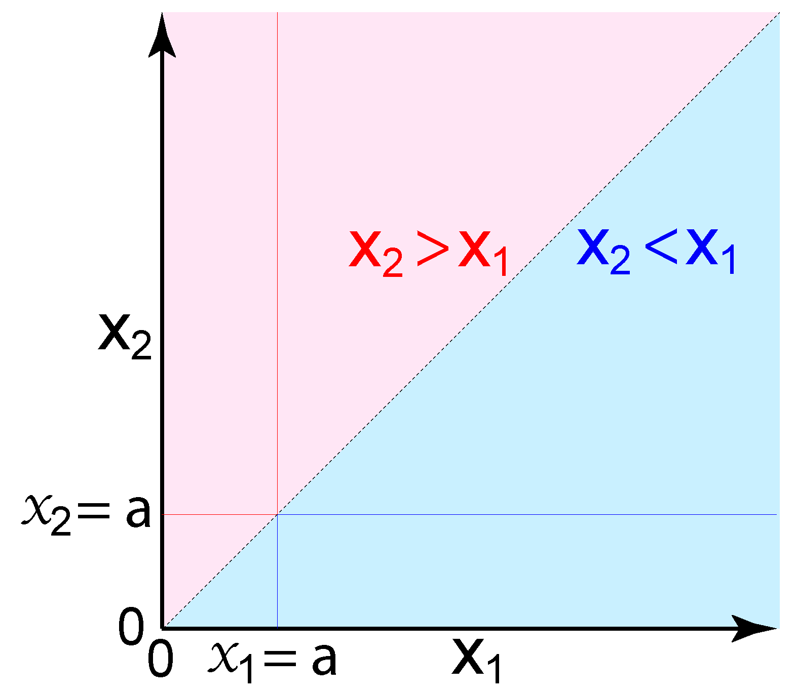
where and are positive and finite real numbers that exhibit a statistical dependence , and there is no additional information that is relevant to probability. These variables could represent physical sizes or magnitudes, such as distances, volumes, or energies. Given only one known size (a sample), what is the probability that an unknown size is larger versus smaller? The answer is not obvious, since there are infinitely more possible sizes corresponding to ‘larger’ than ‘smaller’ (Figure 1).
That such a basic question does not already have a recognized answer is explained not by its mathematical difficulty, but by the remarkable controversy that has surrounded the definition of probability over the last century. We cannot hope to overcome longstanding disputes here, but we try to clarify issues essential to our conclusion (at the cost of introducing substantial text to what would otherwise be concise and routine mathematics).
The question we pose does not involve any frequency; thus it is entirely nonsensical if probability measures frequency. The “frequentist” definition of probability dominates conventional statistics. It was promoted by Fisher and others in an effort to associate probability with objectivity and ontology, but it has severe faults and limitations [1]. We follow instead the Bayesian definition, in which probability concerns prediction (inference) and information (evidence) and epistemology.1
A precise definition of Bayesian probability requires one to specify the exact mathematical relation used to derive probability from information (using criteria such as indifference, transformation invariance, and maximum entropy). This divides Bayesians into two camps. The “objectivists” consider the relation between information and probability to be deterministic [1,2,3,4,5,6,7,8,9,10,11,12], whereas the “subjectivists” consider it to be indeterminate [13,14,15,16,17,18,19,20] (for discussion, see References [1,11,12,17]). We follow the objective Bayesian approach, developed most notably by Jeffreys, Cox, and Jaynes [1,2,3,4,5,6,7].
All Bayesians agree that information is subjective, insofar as it varies across observers (in our view, an observer is information, and information is matter, therefore being local in space and time). The objectivists consider probability to be objective in the sense that properly derived probabilities rationally and correctly quantify information and prediction, just as numbers can objectively quantify distance and energy. Therefore, once the information in our propositions (e.g., ) is rigorously defined, and sufficient axioms are established, there should exist a unique and objectively correct probability that is fully determined by the information. In contrast, subjective Bayesians do not accept that there exists such a uniquely correct probability [13,14,16,17,18,20]; therefore they are predisposed to reject our conclusion.2
Objectivity requires logical consistency. All rigorous Bayesians demand a mathematical system in which an observer with fixed information is logically consistent (e.g., never assigns distinct probabilities to the same proposition). However, subjectivists do not demand logical consistency across observers (Section 3.2). They accept that a Bayesian probability could differ between two observers despite each having identical evidence (see Reference [14], pp. 83–87). In that sense, they see probability as a local and personal measure of evidence, with the relation of probability to evidence across observers being indeterminate. In contrast, the objective Bayesian ideal is a universal mathematics of probability in which the same rules apply to all observers,3 so that probability measures evidence, and evidence uniquely determines probability.
The objective ideal can only be achieved by adopting a sufficient set of axioms (Section 3). We see failure to do so as the critical factor explaining why subjectivists believe the relation between information and probability to be indeterminate (Section 3.2). A mathematical system must be defined by axioms that are neither proven nor provable (they cannot be falsified). For example, there are axioms that define real numbers, and Kolmogorov’s axiom that a probability is a positive real number. These axioms are subjective insofar as others could have been chosen, and there is not a uniquely correct set of axioms.4 There may be any number of axiomatic systems that are each internally consistent and able to correctly (objectively) measure evidence across all observers. We believe the system of Jeffreys, Cox, and Jaynes to be one of these. Thus, we deduce from our axioms, but we do not claim that our axioms are uniquely correct. We claim only that they are commonly used and useful standards.
We are interested in knowledge of only a single ’sample’ because we believe it to be a simple yet realistic model of prediction by a physical observer, such as a sensor in a brain or robot (Section 10) [21,22]. Jaynes often used the example of an “ill informed robot” to clarify the relation of probabilities to information [1]. Unlike a robot, a scientist given only one sample can choose to collect more data before calculating probabilities and communicating results to other scientists. In contrast, a robot must continually predict and act upon its dynamically varying environment in “real time” given whatever internal information it happens to have here and now within its sensors and actuators. If the only information in a sensor at a single moment in time is a single energy , then the probability that an external or future energy is larger must be conditional on only , as expressed by . At that moment, is fixed, and it is not an option for the sensor to gain more information or to remain agnostic. This example helps to clarify the role of probability theory, for which the fundamental problem is not to determine what the relevant information is, or should be, but rather to derive probabilities once the information has been precisely and explicitly defined.
2. Notation
We use bold and stylized font for variables (samples) , and standard font for their corresponding state spaces (note that these are not technically “random variables”; see Section 4.2). Therefore is an element from the set of real numbers (). Whereas these represent dependent variables, are independent of one another (Section 6.3). The subscripts are arbitrary and exchangeable labels; therefore the implication of a sequence is an unintended consequence of this notation.
We denote arbitrary numbers . For each uppercase letter representing real-numbered “location”, we have a corresponding lowercase letter representing a positive real “scale”, (Section 4.2). Therefore lowercase letters symbolize positive real numbers (except , which symbolizes a physical size and is not a number).
As described in Section 4, all probabilities are conditional on prior information I and J, as well as K in cases involving both and (e.g., and ). For simplicity, this conditionality is not shown in notation.
We use uppercase P for the probability of discrete propositions, with defined intervals, , as in the case of a cumulative distribution function (CDF). We use the lowercase p for a probability density function (PDF), which is the derivative of its corresponding CDF, . Because our simplified notation omits the variable of interest and the propositions, for clarity, we define it for CDF and PDF as
where represents the set of possible values of the number ; thus represents an infinite set of propositions, one for each real number. For example, if we had discrete units of 0.1 rather than continuous real numbers, then , . Analogous notation applies to locations; thus, .
A joint distribution over two variables is a marginal distribution of the full joint distribution (following the sum rule),
where n approaches infinity. Likewise, is a marginal distribution of .
3. Axioms
Like other Bayesians, we take as axioms the product and sum rules of Cox (the product rule being Bayes’s Theorem), and Kolmogorov’s first axiom that a probability is a positive real number [1,4,5]. Kolmogorov’s second and third axioms together stipulate that a mutually exclusive set of probabilities must sum to one. Like Cox and Jaynes, we apply this normalization rule where convenient (including the conclusion in our title). However, we do not elevate it to an axiom, since to do so would be unnecessarily restrictive and inconvenient (see Reference [11]).
3.1. Axioms Determine the Non-Informative Prior Distribution
Since we choose to quantify a physical size using a real number , we need axioms that define real numbers. In particular, we need to measure the size of a subset of real numbers (a partition of the state space). For this, we would like to have a volume or integral that is invariant (a Haar measure) under addition (translation invariance; see Section 5). Since our particular interest concerns metric spaces, this Haar measure is essentially the same as a distance metric. We, therefore, choose our measure in one dimension to be the standard distance metric, which is almost universally assumed when using real numbers.
Thus the (uncountable) “number” of values could take between A and B is . We must also specify probability as a function of distance. Our probability measure need not necessarily be the same as our distance measure, as a matter of logic. However, the obvious choice is to equate them, so that the probability that lies within a distance will be that distance. For ,
We declare Equations (5) and (6) to be axioms. These may be seen as innocuous and trivial, but by explicitly asserting them to be axioms, we eliminate the appearance of indeterminacy that underlies the subjectivist view.
The axiom in Equation (6) can be expressed as a cumulative distribution , or in our more concise notation, (Equation (2)). Its derivative is the uniform density, (Equation (3)) (Section 6.1). This is known as a “non-informative prior” (or “reference prior” or “null distribution”), a term for probabilities that are, or are intended to be, conditional on a complete absence of information. Although the uniform prior has long been used, it is the only portion of our proofs that has been a matter of controversy, as we discuss next.
3.2. Controversies Concerning the Uniform Distribution
Whereas we have derived the uniform prior over real numbers, , from the standard distance metric, it has long been justified by “the principle of indifference”. We state this principle as the choice to represent equal evidence with equal probabilities, together with the rationale that a complete absence of evidence must correspond to equal evidence for each proposition (we treat each possible number equally). Although this principle has always been used, it has long been alleged to result in logical contradictions [23]. Whereas indifference only applies in the complete absence of evidence, alleged counterexamples invariably and unwittingly depend upon implicit evidence that discriminates amongst propositions and results in non-uniformity once properly utilized [1,9,24]. An example arises here because we consider two alternative numerical representations (parameterizations) of the same size, and (Section 4.2). Assigning uniformity over both and would result in logical contradictions. Instead, we begin with axioms that assign uniformity over , and then introduce information , so that is not uniform (Section 6.2).
Subjectivists have defended use of the uniform prior as a practical matter but have argued or implied that uniquely correct non-informative priors do not exist [13,14,16,17,18]. Objectivists have argued that the uniform prior is uniquely correct in the absence of information [1,2,3,9,11]. Here, we resolve this issue, at least as a practical matter, by declaring the standard distance metric and the uniform density as axioms. These axioms may be “uniquely correct” in the sense that they are the least complex and most convenient. However, we have no need to make that claim, and simplicity and convenience are not essential to an objective and logically consistent mathematics of probability. (see footnote 4).
Specifically, subjectivists have criticized the uniform prior on the grounds that it is not uniquely correct because, whether one derives uniformity from the principle of indifference or location invariance (Equation (16)), it has the general form , where c is any positive constant. Thus, the non-informative prior appears indeterminate, and if different observers choose different values of c, there will appear to be logical inconsistency across observers (see Reference [14], pp. 83–87). This trivial but undesirable sort of subjectivity is analogous to one observer choosing the metric system and another the English system of measurement. It is overcome by adopting an axiom that fixes c as a universal constant to apply to all observers. We have achieved the same end merely by declaring the standard distance metric an axiom, from which we deduce (Section 3.1). Our proofs would be unaltered were we to choose any specific constant . However, would be formerly equivalent to defining a non-standard distance metric, .
The uniform density has also caused confusion because it is unnormalizable (“improper”) and hence not a “probability” as defined by Kolmogorov’s axioms (Section 3). The semantic issue of whether to denote the function a “probability” is not critical (we do, but Norton does not [9]). The deeper issue concerns the rationale for, and form of, normalization. In geometry, one can only assign a number to a single distance between points in an arbitrary manner. The assignment of ‘1’ to ‘a meter’ is convenient but is otherwise arbitrary and meaningless. Numbers acquire meaning in applied mathematics only when there is a ratio of two sizes. Thus ‘8 m’ represents, by definition, the ratio 8/1. The numerator and denominator are each arbitrary and meaningless in isolation, but the ratio is not; therefore science measures relative size as ratio (or log ratio). The same applies to probability, as in , which has a perfectly clear meaning, even though both numerator and denominator are each “improper probabilities” that mean nothing in isolation. Whereas this ratio compares the probability of one ‘part’ to another, the standard ratio that has been chosen by convention to define a “proper probability” is ‘part / whole’, , where ‘+’ and ‘−’ indicate true and false propositions. Kolmogorov elevated this form of normalization to an axiom, but, like Cox and other objective Bayesians, we do not [1,4,5]. However, the conditional probabilities that are our ultimate interest, , do normalize in the conventional manner, since, although the numerator and denominator on the right are each “improper” (unnormalizable), the conditional probability is their ratio and is a properly normalized density.
4. Defining the Prior Information
We try to define the prior information as rigorously and explicitly as possible, since failure to do so has been a major source of confusion and conflict regarding probabilities. We distinguish information I about physical sizes, information J about our choice of numerical representation of size (the variables), and information K about the statistical dependence between variables. For clarity, we also distinguish the prior information from its absence (ignorance). Although it is the information that we seek to quantify with probabilities, it is its absence that leads directly to the mathematical expressions of symmetry that are the antecedents of our proofs.
4.1. Information I about Size
Information I is prior knowledge of physical ‘size’. Our working definition of a ‘size’ is a physical quantity that we postulate to exist, such as a distance, volume, or energy, which is usually understood to be positive and continuous. A ‘size’ need not have extension and is not distinguished from a ‘magnitude’. Critically, since a single size can be quantified by various numerical representations, and size is a relative rather than absolute quantity, a specific size is not uniquely associated with a specific number, and the space of possible sizes s is not a unique set of numbers. Information I concerns only prior knowledge of physical size , not its numerical representation (such as ).
We define I as the conjunction of three postulates.
- There exist a finite and countable number of distinct sizes .
- Each existing size is an element of a totally ordered space of possible sizes s.
- For each existing size , there are larger and smaller possible sizes within s.
Information I is so minimal that it could reasonably be called “the complete absence of information”. Being so minimal, I appears vague, but its consequence becomes more apparent once we consider its many corollaries of ignorance. These constrain our choice of numerical representation (Section 4.2) and provide the sufficient antecedents for our proofs (Section 4.4).
4.2. Information J about Numerical Measures of Size
We should not confuse our information I about physical sizes with our information J about our choice of numerical representation. J corresponds to our knowledge of numbers, which includes our chosen axioms. We will therefore use the term “size” for a physical attribute, and “variable” for a number we use to quantify it (we quantify size with variables and ). Our choice of numerical representation J cannot have any influence on the actual sizes, or our information I about them; thus probabilities must be invariant to our choice of numerical representation (parameterization) (Section 5.1) (although the density does depend on J).
Information I implies certain properties that are desirable if not necessary in our choice of J. Postulate 1 indicates that there must be an integer number of sizes (samples) that actually exist, . Since no number is postulated, n is unknown, and its state space is countably infinite. For example, each size could be the distance between a pair of particles, and the number of pairs n is unknown. For each of these n sizes, we define below two corresponding numerical quantities (variables). Postulate 2 specifies no minimal distance between neighboring sizes in the ‘totally ordered space’ s; thus s is continuous. Postulate 3 specifies that, for any given size , larger and smaller sizes are possible. Thus, no bound is known for space s, and the range of possibilities is infinite. We therefore choose to represent a physical size with real numbered variables ( and ), with more positive numbers representing larger sizes. We emphasize that, although the true value of each variable is finite, that value is entirely unknown given prior information I and J; therefore its state space is uncountably infinite.
We choose two numerical representations, one measuring relative size as difference, and the other as ratio, related to one another by exponential and logarithmic functions.
We define information J as the conjunction of these equations, together with the standard distance metric in one dimension.
We therefore represent a single physical size with two numbers (variables), “scale” and “location” , where . In common practice, a “scale” typically corresponds to a ratio (e.g., m is the ratio , by definition); therefore, a “location” corresponds to a log ratio, . Because we are free to choose any parameterization, and only one is necessary for a proof, it is not essential that we justify the relationship between parameterizations. However, the exponential relationship arises naturally and is at least a convenient choice.5
Since we follow the objective Bayesian definition of probability, our variables are not “random variables” in the standard sense (see Reference [1], especially p. 500). This is in part just semantic, since “random” is ill-defined in standard use and promotes misunderstanding. The technical distinction is that the standard definition of a “random variable” assumes there to be a function (known or unknown) that “randomly samples” from its state space following some “true probability distribution” (which could be determined by a physical process). We do not assume there to be any such function or true distribution. Information I and J leaves us entirely agnostic about any potential process that might have generated the physical size we quantify with . Such a process could just as well be deterministic as random, and even if we knew it to be one or the other, this alone would not alter the probabilities of concern here.
4.3. Information K about Dependence of Variables
Information K postulates that the variables are not independent but does not specify the exact form of dependence. The dependence between variables is typically specified as part of a statistical model. It relates to a measure of the state space in two or more dimensions. For example, the Euclidean distance metric, which exhibits rotational invariance, underlies what we call “Gaussian dependence”.
For independent variables and , , and therefore our conclusion that is obvious (although since is not normalizable, is not a unique median). Given our measures of distance (Equation (5)) and probability (Equation (6)) in one dimension, the measure in this two-dimensional state space is simply the product
where is the joint CDF in our simplified notation (Equation (2)). Information K postulates a dependence, which we define by the negation of Equation (11):
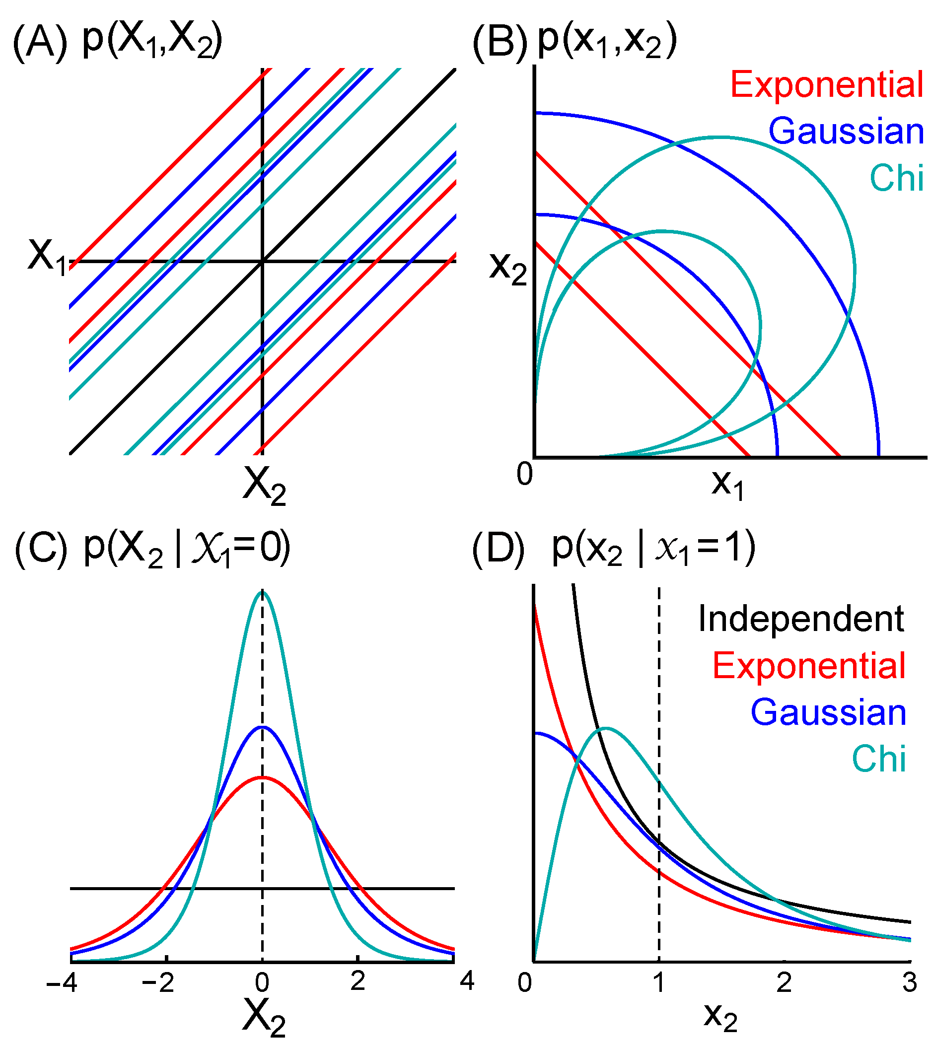
We further define K to be any form of dependence (measure) consistent with the two corollaries specified below that result from the conjunction of information I, J, and K (Section 4.4). These corollaries mandate symmetries (Section 5) that defines a set of joint distributions and . Our proofs apply to every member of this set. They demonstrate that every member of the set has the form , where h is any function consistent with our corollaries. Figure 2 illustrates three exemplary distributions in set . In Section 7, we present in detail the special case of an “exponential” dependence or model.
4.4. Corollaries of Ignorance Implied by I, J, and K
The conjunction of information I, J, and K is all prior knowledge, and its logical corollary is ignorance of all else. The consequence of ignorance is symmetry, which provides constraints that we use to derive probabilities.
Corollary.
There is no information beyond that in I, J, and K.
- 1.
- There is no information discriminating the location or scale of one variable from another.
- 2.
- There is no information about the location or scale of any variable.
Corollaries 1 and 2 make explicit two sorts of ignorance that are necessary and sufficient for our proofs. Corollary 1 requires that we treat variables equally, meaning that they are “exchangeable” (Equation (14)). Corollary 2 is sufficient to establish location and scale invariance (Equations (15)–(18)) and to derive non-informative priors over single variables (Equations (19)–(22)).
5. Invariance of Prior Probabilities
Given the minimal information defined above, prior probabilities must be invariant to the choice of parameters, exchange of variables, and changes to location and scale [1,2,3,8,9,10,11,13,14,16,26,27,28,29].
5.1. Invariance to Change of Parameters
Probability must not vary with our choice of parameters (Section 4.2). Therefore,
where the left and right sides represent size as locations and scales, respectively, related by . These probabilities are equal because these are two distinct formulations of the same proposition (this invariance does not extend to densities and , which have different domains, and thus different forms).
5.2. Exchangeability of Variables
Corollary 1 requires that we treat all variables equally. Therefore must exhibit “exchangeability of variables,”
for all positive numbers a and b. Exchangeability corresponds to symmetry of around the identity line, (Figure 1 and Figure 2B), and likewise for (Figure 2A). Here, we show only two variables, but exchangeability applies to all n variables in the joint distribution . Although n will be finite, it is unknown and unbounded (Section 4.1, postulate 1); we therefore consider the consequences of allowing n to approach infinity. As a result, we have “infinite exchangeability” of variables and can use de Finetti’s theorem, which ensures the existence of a set of parameters that, if known, cause the variables to be independent and identically distributed (i.i.d.) (see Section 8.3) [13,16,26] (see Chapter 4.3.3 in Reference [16]).
5.3. Location and Scale Invariance
Since corollary 2 stipulates no prior information about size, the prior probability that lies in an interval must be invariant to a change in the location of that interval (as in choosing a different origin). Therefore, we have location (translation) invariance
for any number . We can express this instead as integrals over densities, , or
Because we must have invariance to a change of parameters (Equation (13)), we can rewrite Equation (15) given , so that location invariance becomes scale invariance
Therefore , and scale invariance with respect to densities is
6. Prior Probabilities over Single Variables
6.1. The Prior over Locations
We express the non-informative prior over location (Equation (6)) more concisely as a CDF (following Equation (2)),
and its derivative, the uniform PDF
The uniform density is unique in exhibiting location (translation) invariance (Equation (16)), which provides an alternative derivation of it as the non-informative prior over real numbers [1,2,3]. Note that, since we derived the uniform prior from the standard distance metric (Equation (5)), it also applies to a positive variable, .
6.2. The Prior over Scales
Because the non-informative prior over scale is less obvious than the uniform prior, we provide three derivations of it. First, because probabilities must be invariant to a change in parameters (Equation (13)), we can find the prior over scales simply by transforming locations, (Equation (8)) (see Reference [14], p. 82). Therefore, (Equation (6)) becomes , and the CDF is
and the corresponding PDF is
A second and more famous derivation is based on the fact that , where is a constant, is the unique distribution that exhibits the scale invariance defined by Equation (18) [1,2,3]. The value of c is irrelevant to our proofs (Section 6.4), but is implied by Equations (19), (20), and Equation (8). Thus we have Equation (22), known as “Jeffreys prior over scale” (which applies whether the unknown is called a “scale parameter” or “variable”). A third derivation below considers a ratio of independent variables.
6.3. Independence and the Prior over Differences and Ratios
The priors over single variables derived above are sufficient for our proofs. However, we can gain additional insight by deriving the non-informative prior over difference and ratio. Complete absence of information requires that we do not have information K (Section 4.3) specifying a dependence, and instead have independent variables .
Given the joint CDF (Equation (11)), the joint PDF is uniform, ; therefore uniformity applies to all sums and differences,
which are also independent of one another. Transforming locations to scales (Equations (8) and (13)), we have the analogous equation , and the product is independent of ratios and . Thus non-informative priors over products and ratios, and sums and differences, have the same form as shown above for scales and locations, respectively. Indeed, we introduce no information about location or scale if we define and , and all numbered equations remain valid if we do so.
6.4. The Uniform Prior over Positive Variables
Here, we derive Jeffreys non-informative prior over scale (Equations (21) and (22)) from the uniform prior over positive and independent real numbers. Although less formal than the derivation above (Section 6.2), this derivation may be more appealing conceptually to some since it does not rely on negative numbers and the exponential function.
We begin with uniformity and independence of positive variables, . This gives (Equation (23)), and exchangeability (Equation (14)) requires . Combining these, we have for the subset of propositions , . This is easily seen to correspond to uniform density over the logarithm, (‘1’ is required by Equation (5), but any constant is sufficient for present purposes). By defining and , this becomes (Equation (20)), which we have shown above to be sufficient to derive (Equation (19)) and (Equation (22)) (Section 6.2). Therefore Jeffreys’s prior over scale (Equation (22)) is the distribution over a ratio of two independent and uniformly distributed positive real numbers.
This derivation appears to have failed to account for the possible combinations of and . For example, it would appear that a ratio ‘1’ could be achieved by any element of the set ‘1/1’, ‘2/2’, ‘3/3’,..., whereas a more extreme ratio, such as ‘1/527’, can be achieved only by a smaller set of combinations. However, the apparent multiplicity of combinations (degeneracy) is illusory here, a counter-intuitive property of independence and a complete absence of information. For example, rather that representing a distance between two geometric points with a single number , we could represent it by assigning two arbitrary numbers and to the two points, so that . The question then arises whether combinations of ‘’, such as ‘’ and ‘’, are distinguishable (degenerate) states, or indistinguishable states (Bose-Einstein statistics being a consequence of the latter). If one postulates that a single distance is associated with a uniquely correct number, but a single geometric point can only be assigned a number arbitrarily (as typically implied in trigonometry, in which similar triangles of different scales are distinguished, but identical triangles in different locations are not), then ‘’ and ‘’ are not distinguishable states, and there is only one way to achieve one distance . Thus, the state space ‘’, like that of , is effectively one-dimensional. Choosing to parameterize with ‘’ creates what could be called “pseudodegeneracy”, since we cannot expand the size or dimensionality of a state space by choosing to introduce a superfluous and potentially misleading variable. This contrasts with our case of dependent variables and , for which we treat ‘’ and ‘’ as two distinct combinations.
7. Exemplary Case of an Exponential Dependence
Before general proofs, we present here examples of dependence, and we summarize each of our three proofs for the special case of an “exponential” dependence or model.
7.1. Three Exemplary Forms of Dependence
Figure 2 shows distributions for three forms of dependence in set (Section 4.3). The joint distribution over two variables given an exponential dependence is
whereas “Gaussian” and “chi” dependence yields and , respectively. Transformation of Equation (24) according to (using Equation (13) after converting from PDF to CDF) gives
The sufficient statistic for the exponential model given samples and is , and the scale parameter given an infinite “population” of samples is . If is known, the sampling distribution is “the exponential distribution”, . Therefore, we refer to this dependence (or statistical model) as ‘exponential’, even though is unknown in our case (we have a non-informative prior over ). We apply the same rationale in denoting our “Gaussian” and “chi” dependencies.
7.2. Proofs 1 and 2 Given Exponential Dependence
If is known, Equation (24) becomes (given the product rule , and ). Its integral is the CDF , proving that is the median (Equation (1)). This distribution is known as‘log-logistic’ with scale parameter and shape parameter 1. However, proofs 1 and 2 take advantage of the greater symmetry present in compared to (although proof 2 begins with the latter). Logarithmic transformation converts the log-logistic distribution to the logistic distribution (Equation (25)), with location parameter and scale parameter 1. It can readily be shown that (Figure 2A,C), indicating that the logistic distribution is an even function, . Therefore, is its median, as well as mean and mode. Since the median is invariant to a change of parameters (Equation (13)), is the median of the log-logistic distribution.
7.3. Proof 3 Given Exponential Dependence
Proof 3 uses the “population” scale parameter , for which the sampling distribution is the exponential distribution, . From this and the prior over a scale parameter (Section 6.2), the posterior predictive distribution is
which is again the log-logistic distribution (Section 7.2) (Figure 2B,D). The median is , since . One can use the same approach to confirm that this is also true given any particular statistical model of positive real variables that is famous enough to have a name (e.g., gamma, chi, half-normal), so long as there is no prior information about scale (as in the case that .
8. General Proof
Proofs 1–3 all proceed from corollary 1, expressed in exchangeability (Equation (14)), and corollary 2, expressed in location and scale invariance (Equations (15)–(18)), and prior probabilities (Equations (6) and (19)–(22)). Proof 1 starts by observing that must be an even function. Proof 2 applies scale invariance across all dimensions of . Proof 3 uses a scale parameter that renders the variables conditionally independent and identically distributed (i.i.d.). Proof 1 is the simplest and proof 3 the most complex. It is interesting to note that we derived them in the opposite order chronologically, which is explained primarily by the fact that proof 3 uses the most common Bayesian methods.
We also note that proofs 2 and 3 begin with strictly positive numbers , and proof 3 never uses negative numbers. Furthermore, whereas we chose to present our axioms using the standard distance metric for all real numbers (locations), scale invariance (Equation (18)) is an alternative antecedent for our proofs. It can be understood as the consequence of beginning with a multiplicative metric, rather than the standard metric based on difference.
8.1. Proof 1 from the Joint Distribution
To characterize , it is useful to consider sums and differences, and (note that corresponds to rotating by 90 degrees). Given exchangeability (Equation (14)) from corollary 1, must be evenly distributed around the identity line for all forms of dependence (statistical models) in set , so that it is invariant to exchange of and . Therefore,
which must be an even function, .
Given corollary 2, we know nothing about the location of either or , and knowing that they exhibit a dependence contributes no information about their joint location (Section 4.3). Therefore, we know nothing about their sum, resulting in uniformity,
so that all lines through perpendicular to the identity line are equally probable, . Uniformity over sums (Equation (28)) is easily seen to be a consequence of location invariance (Equation (16)), since (Equation (20)), and we must have invariance of the distribution whether we add to either an arbitrary number C or location .
The combination of Equations (27) and (28) requires that must be a function only of the difference between variables for every statistical dependence (model) in set ,
meaning that equiprobability contours must be parallel to the identity line, as shown in Figure 2A.
Given a known sample , the conditional distribution is a slice through perpendicular to the axis. It can be seen in Figure 2A that the distribution over the difference is identical for all values of .
This proves that and have no information about one another and are therefore independent. From this and Equation (27), must be an even function with median (Figure 2C), proving our conclusion
Converting to scales (Equations (8) and (13)) shows that and must also be independent, and proves our conclusion that a known positive variable is the median over an unknown.
The conclusion in our title, that these probabilities equal , will be true only if has a finite integral (is normalizable). All forms of dependence of which we are aware do result in normalizable conditional distributions, but we do not rule out the possibility of a dependence in set that is an exception. If there is such a case, equations Equations (31) and (32) remain valid, but there will be no unique median.
8.2. Proof 2 from the Joint Distribution
The prior over scales (Equation (22)) can be derived as the unique distribution exhibiting invariance following scale transformation (Equation (18)), exemplifying the method of “transformation groups” [1,8,9,10,11,27,28,29]. Here we transform the scale of all variables simultaneously
where . This requires that the joint distribution exhibit a symmetry that could be termed “multidimensional scale invariance”, so that (where subscript ‘1’ is exchangeable with any other subscript). It is also sufficient to ensure that the joint distribution is a homogeneous function, so that multiplying each variable by c is equivalent to dividing the joint distribution by ,
We define the set of joint distributions to be those that satisfy both this multidimensional scale invariance (Equation (34)) and exchangeability (Equation (14)). We can find a general form for the set by first applying Euler’s homogeneous function theorem to Equation (34). In the case of two variables, this gives
and the general solution is , where and are two arbitrary functions. Whereas this equation was deduced solely from scale invariance (Equation (34)) (required by corollary 2), we next apply exchangeability of variables (Equation (14)) (required by corollary 1). This shows that , and likewise for , so that . Thus there is only one arbitrary function, , and the general solution for two variables becomes
where is any arbitrary function that satisfies this equation. We can find the general form of by dividing Equation (36) by (Equation (22)), which yields
Following logarithmic transformation , this becomes
8.3. Proof 3 from a Scale Parameter
Because of corollary 1, we have exchangeability (Equation (14)), and the theorem of de Finetti ensures the existence of a set of parameters that, if known, renders the variables independent and identically distributed (i.i.d.) (Section 5.2).
This set will include a scale parameter6 , and the non-informative prior will be (Section 6.2). We denote other parameters in set as , so that . The posterior predictive distribution can be expressed as
The general form of , which can be found using the method of transformation groups [1], is
where is an arbitrary normalizable function, the specific form of which depends on the types and values of parameters in (for example, the exponential distribution or gamma distribution ).
The remaining terms in Equation (40) are and . As a scale parameter, in Equation (41) determines only the width of the distribution, and is not informative with respect to its shape, which is determined by . Thus, and are independent such that . We need not assume anything about the form of , except that it normalizes so that .7
All terms in Equation (40) are now determined. Using the fact that , where is the cumulative distribution of , and by substituting , the median of the predictive distribution is
Since , it can be shown that . The same procedure can be used to demonstrate . This proves our conclusion
where ‘1/2’ applies because we have assumed in proof 3 that is normalized (see Section 8.1).
9. The Effect of Additional Information
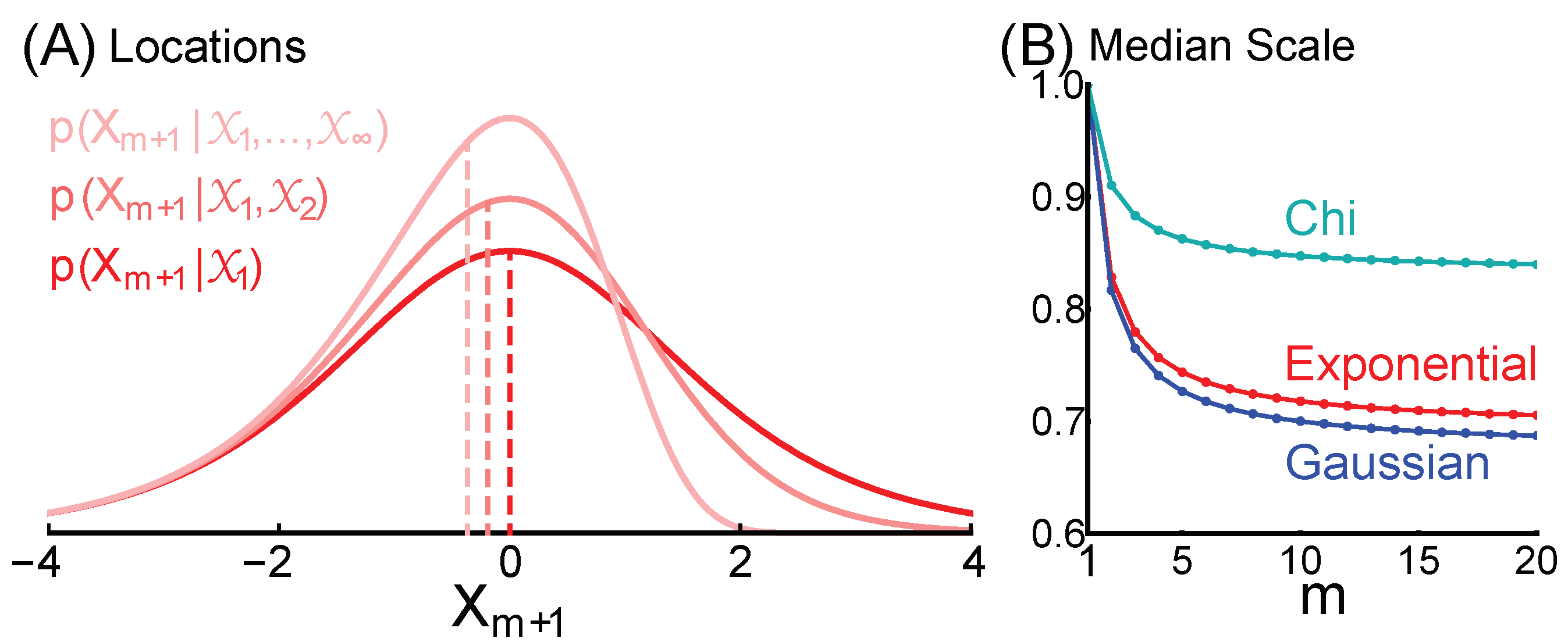
A single known number is the median over an unknown only as a result of ignorance (corollaries 1 and 2), and therefore additional information can result in loss of this symmetry. For example, is not the median of if and . This is because and are not exchangeable in the joint distribution . An interesting special case is that m variables are known and are equal to one another, . One might expect that the median will be the one known number, but this is only true if , at least for our exemplary forms of dependence. Scale information increases with m, causing the distribution to skew towards smaller numbers (Figure 3A). If , the median converges to a number between 0 and 1 that is determined by the form of dependence (Figure 3B). Given the exponential dependence, the median is , which is ≈ 0.828 for , and converges to as m goes to infinity.
There are forms of additional information that allow a single known to remain the median. For example, additional information could specify that and are each the mean or sum of m variables.8 We still must treat and equally, and we still know nothing about their scale; therefore, is still the median of . This remains true whether the number of summed variables m is itself known or unknown.
10. Discussion
Our proof advances the objective Bayesian foundation of probability theory, which seeks to quantify information (knowledge or evidence) with the same rigor that has been attained in other branches of applied mathematics. The ideal is to start from axioms, derive non-informative prior probabilities, and to then deduce probabilities conditional on any additional evidence. A probability should measure evidence just as objectively as numbers measure physical quantities (distance, energy, etc.).
The only aspect of our proofs that has been controversial is the issue of whether absence of information uniquely determines a prior distribution over real numbers. Formal criteria, including indifference, location invariance, and maximum entropy, have all been used to derive the uniform density , where (Section 6). Subjectivists view c as indeterminate, thus being a source of subjectivity (see Reference [14], pp. 83–87), whereas objectivists view it merely as a positive constant to be specified by convention (our proofs hold for any choice of c). In contrast, we deduced from the standard distance metric, which we declared an axiom (Equation (5)) (Section 3). In our opinion, the indeterminacy of the subjectivist view is the logical result of insufficient axioms.
Our conclusion appears surprising, since for any known and finite positive number, the space of larger numbers is infinitely larger than the space of smaller positive numbers (Figure 1). However, probability measures evidence, not its absence, and the space of possibilities only exists as the consequence of the absence of evidence (ignorance). A physical ‘size’ is evidence about other physical sizes, and we postulate that physical size and evidence exist (Section 4.1). This postulate implies that the absence of evidence (ignorance), and the corresponding state space, does not exist (or at least has a secondary and contingent status) and therefore carries no weight in reasoning. Reason requires that two physical sizes be treated equally (Section 4.4), and there is no evidence that one is larger than the other, even if one is known. In this way our proof that a known number (quantifying size) is the median over an unknown can be understood intuitively. Our result can also be understood by considering that there is no meaningful (non-arbitrary) number associated with a single “absolute” size (Section 3.2), but only with ratios of sizes, and we must have (Section 6.4), regardless of whether is known. Indeed, we have proven that has no information about or , and vice versa (Section 8.1), even though and are dependent variables and thus have information about one another.
Practical application of our result requires us to consider what information we actually have. The probability that the unknown distance to star B is greater than the known distance to star A is , and the probability is also that the unknown energy of particle B is greater than the known energy of particle A. However, this is only true in the absence of additional information. We do realistically have additional information that is implicit in the terms ‘star’ and ‘particle,’ since we know that the distance to a star is large, and the mass of a particle is small, relative to the human scale. Before inquiring about stars or particles, we already know the length and mass of a human, and that additional information changes the problem. Furthermore, we know the human scale with more certainty than we can ever know a much larger or smaller scale.
All scientific measurement and inference of size begins with knowledge of the human scale that is formalized in our standard units (m, kg, s, etc.). These standard units are only slightly arbitrary, since they were chosen from the infinite space of possible sizes to be extremely close to the human scale. Therefore members of the set of distributions that we have characterized here, each conditional on one known size, would be appropriate as prior distributions given only knowledge of standard units. One meter would then be the median over an unknown distance . If is then observed, and we ask “what is another distance ?”, we already know two distances, and neither will be the median (our central conclusion does not apply) (Figure 3) (Section 9).
A beautiful aspect of Bayesian probabilities is that they can objectively describe any knowledge of any observer, at least in principle. Probabilities are typically used to describe the knowledge of scientists, but they can also be used to describe the information in a cognitive or physical model of an observer. This is the basis of Bayesian accounts of biology and psychology that view an organism as a collection of observers that predict and cause the future [21,30,31,32,33,34,35,36,37,38,39,40].
All brains must solve inference problems that are fundamentally the same as those facing scientists. When humans must estimate the distance to a visual object in a minimally informative sensory context, such as a light source in the night sky, they perceive the most likely distance to be approximately one meter, and bias towards one meter also influences perception in more complex and typical sensory environments [41,42]. This is elegantly explained by the fact that the most frequently observed distance to visual objects in a natural human environment is about a meter [31]. The brain is believed to have learned the human scale from experience, and to integrate this prior information with incoming sensory ‘data’ to infer distances, in accord with Bayesian principles [30,31,32]. Therefore, a simple cognitive model, in which the only prior information of a human observer is a single distance of m, or an energy of joule (kg m2 s−2), might account reasonably well for average psychophysical data under typical conditions.
Such a cognitive model is extremely simplified, since the knowledge in a brain is diverse and changes dynamically over time. However, we do not think it is overly simplistic for a model of a physical observer to be just a single quantity at a single moment in time. The brain is a multitude of local physical observers, but our initial concern is just a single observer at a single moment [21,22,33,34,35]. The problem is greatly simplified by the fact that we equate an observer with information, and information with a physical quantity that is local in space and time, and is described by a single number. For example, a single neuron at a single moment has a single energy in the electrical potential across its membrane.9 Given this known and present internal energy, what is the probability distribution over the past external energy that caused it, or the future energy that will be its effect? Here, we have provided a partial answer by characterizing a set of candidate distributions, and demonstrating that a known energy will be the median over an unknown energy.
Author Contributions
In chronological order, C.D.F. conceived the hypothesis, S.L.K. derived proof 3 and then proof 2, C.D.F. derived proof 1, C.D.F. wrote the original manuscript, and C.D.F. and S.L.K. edited the manuscript. All authors have read and agreed to the published version of the manuscript.
Funding
This research was funded by a grant to C.D.F. from the National Research Foundation of the Republic of Korea (N01200562), and a KAIST Grand Challenge 30 grant (KC30, N11200122) to C.D.F. from KAIST and the Ministry of Science and ICT, Republic of Korea.
Acknowledgments
We thank Jaime Gomez-Ramirez for helpful discussions and comments on an early version of the manuscript.
Conflicts of Interest
The authors declare no conflict of interest. The funders had no role in the design of the study, in either the collection or analyses or interpretation of data, in the writing of the manuscript, or in the decision to publish the results.
References
- Jaynes, E.T. Probability Theory: The Logic of Science; Cambridge University Press: Cambridge, UK, 2003. [Google Scholar]
- Jeffreys, H. On the theory of errors and least squares. Proc. R. Soc. Lond. Ser. A 1932, 138, 48–55. [Google Scholar]
- Jeffreys, H. The Theory of Probability; The Clarendon Press: Oxford, UK, 1939. [Google Scholar]
- Cox, R. Probability, frequency and reasonable expectation. Am. J. Phys. 1946, 14, 1–13. [Google Scholar] [CrossRef]
- Cox, R. The Algebra of Probable Inference; Johns Hopkins University Press: Baltimore, MD, USA, 1961. [Google Scholar]
- Jaynes, E.T. Information theory and statistical mechanics. Phys. Rev. 1957, 106, 620–630. [Google Scholar] [CrossRef]
- Jaynes, E.T. Some random observations. Synthese 1985, 63, 115–138. [Google Scholar] [CrossRef]
- Goyal, P. Prior probabilities: An information-theoretic approach. AIP Conf. Proc. 2005, 803, 366–373. [Google Scholar]
- Norton, J.D. Ignorance and indifference. Philos. Sci. 2008, 75, 45–68. [Google Scholar] [CrossRef] [Green Version]
- Baker, R.; Christakos, G. Revisiting prior distributions, Part I: Priors based on a physical invariance principle. Stoch. Environ. Res. Risk Assess. 2007, 21, 427–434. [Google Scholar] [CrossRef]
- Stern, J.M. Symmetry, invariance and ontology in physics and statistics. Symmetry 2011, 3, 611–635. [Google Scholar] [CrossRef]
- Williamson, J. Objective Bayesianism, Bayesian conditionalisation and voluntarism. Synthese 2011, 178, 67–85. [Google Scholar] [CrossRef] [Green Version]
- de Finetti, B. Probability Theory: A Critical Introductory Treatment; John Wiley & Sons: Chichester, UK, 1975. [Google Scholar]
- Berger, J.O. Statistical Decision Theory and Bayesian Analysis; Springer: New York, NY, USA, 1985. [Google Scholar]
- Howson, C.; Urbach, P. Bayesian reasoning in science. Nature 1991, 350, 371–374. [Google Scholar] [CrossRef]
- Bernardo, J.M.; Smith, A.F. Bayesian Theory; John Wiley & Sons: Chichester, UK, 1994. [Google Scholar]
- Kass, R.E.; Wasserman, L. The selection of prior distributions by formal rules. J. Am. Stat. Assoc. 1996, 91, 1343–1370. [Google Scholar] [CrossRef]
- Irony, T.Z.; Singpurwalla, N.D. Non-informative priors do not exist: A dialogue with Jose M. Bernardo. J. Stat. Plan. Inference 1997, 65, 159–189. [Google Scholar] [CrossRef]
- Howson, C. Probability and logic. J. Appl. Log. 2003, 1, 151–165. [Google Scholar] [CrossRef] [Green Version]
- Berger, J.O.; Bernardo, J.M.; Sun, D. Overall Objective Priors. Bayesian Anal. 2015, 10, 189–221. [Google Scholar] [CrossRef]
- Fiorillo, C.D. Beyond Bayes: On the need for a unified and Jaynesian definition of probability and information within neuroscience. Information 2012, 3, 175–203. [Google Scholar] [CrossRef] [Green Version]
- Kim, S.L.; Fiorillo, C.D. Describing realistic states of knowledge with exact probabilities. AIP Conf. Proc. 2016, 1757, 060008. [Google Scholar]
- Keynes, J. A Treatise on Probability; Macmillan: London, UK, 1921. [Google Scholar]
- Tschirk, W. The principle of indifference does not lead to contradictions. Int. J. Stat. Probab. 2016, 5, 79–85. [Google Scholar] [CrossRef] [Green Version]
- Argarwal, R.P.; Karapınar, E.; Samet, B. An essential remark on fixed point results on multiplicative metric spaces. Fixed Point Theory Appl. 2016, 21, 1–3. [Google Scholar]
- Gelman, A.; Carlin, J.B.; Stern, H.S.; Rubin, D.B. Bayesian Data Analysis; CRC Press: Boca Raton, FL, USA, 2003. [Google Scholar]
- Arthern, R.J. Exploring the use of transformation group priors and the method of maximum relative entropy for Bayesian glaciological inversions. J. Glaciol. 2015, 61, 947–962. [Google Scholar] [CrossRef] [Green Version]
- Terenin, A.; Draper, D. A noninformative prior on a space of distribution functions. Entropy 2017, 19, 391. [Google Scholar] [CrossRef] [Green Version]
- Worthy, J.L.; Holzinger, M.J. Use of uninformative priors to initialize state estimation for dynamical systems. Adv. Space Res. 2017, 60, 1373–1388. [Google Scholar] [CrossRef]
- Weiss, Y.; Simoncelli, E.P.; Adelson, E.H. Motion illusions as optimal percepts. Nat. Neurosci. 2002, 5, 598–604. [Google Scholar] [CrossRef] [PubMed]
- Yang, Z.; Purves, D. A statistical explanation of visual space. Nat. Neurosci. 2003, 6, 632–640. [Google Scholar] [CrossRef]
- Kording, K.P.; Wolpert, D.M. Bayesian integration in sensorimotor learning. Nature 2004, 427, 244–247. [Google Scholar] [CrossRef]
- Fiorillo, C.D. Towards a general theory of neural computation based on prediction by single neurons. PLoS ONE 2008, 3, e3298. [Google Scholar] [CrossRef] [PubMed]
- Fiorillo, C.D.; Kim, J.K.; Hong, S.Z. The meaning of spikes from the neuron’s point of view: Predictive homeostasis generates the appearance of randomness. Front. Comput. Neurosci. 2014, 8, 49. [Google Scholar] [CrossRef] [PubMed] [Green Version]
- Kim, J.K.; Fiorillo, C.D. Theory of optimal balance predicts and explains the amplitude and decay time of synaptic inhibition. Nat. Commun. 2017, 8, 14566. [Google Scholar] [CrossRef] [Green Version]
- Friston, K. The free-energy principle: A unified brain theory? Nat. Rev. Neurosci. 2010, 11, 127–138. [Google Scholar] [CrossRef]
- Harris, A.J.; Osman, M. The illusion of control: A Bayesian perspective. Synthese 2012, 189, 29–38. [Google Scholar] [CrossRef]
- Clark, A. Whatever next? Predictive brains, situated agents, and the future of cognitive science. Behav. Brain Sci. 2013, 36, 181–204. [Google Scholar] [CrossRef]
- Nakajima, T. Probability in biology: Overview of a comprehensive theory of probability in living systems. Prog. Biophys. Mol. Biol. 2013, 113, 67–79. [Google Scholar] [CrossRef] [PubMed]
- Kim, C.S. Recognition dynamics in the brain under the free energy principle. Neural Comput. 2018, 30, 2616–2659. [Google Scholar] [CrossRef] [PubMed]
- Gogel, W.C.; Tietz, J.D. Absolute motion parallax and the specific distance tendency. Percept. Psychophys. 1973, 13, 284–292. [Google Scholar] [CrossRef] [Green Version]
- Owens, D.A.; Leibowitz, H.W. Oculomotor adjustments in darkness and the specific distance tendency. Percept. Psychophys. 1976, 20, 2–9. [Google Scholar] [CrossRef]
| 1. | The relation of Bayesian probability to ontology is irrelevant to our proofs. However, our interest in probability stems from our belief that evidence (information) exists, that it should therefore be intrinsic to ontological and physical models, and that it can be quantified using Bayesian probabilities. |
| 2. | The terms “objective” and “subjective” have had various uses in the Bayesian literature. In contrast to the distinction we make, some subjectivists have used “objective” (or “non-subjective”) to refer to any number purported to be a probability if it is derived by any formal mathematical criterion, regardless of whether that criterion is sensible let alone correct, and “subjective” for any other “probability” (such as a verbally expressed opinion) [18,20]. |
| 3. | That the same rules should apply to all observers is fundamental to physics. Likewise, the objective Bayesian view tends to be more prevalent among physical scientists, and the subjective Bayesian view among social scientists. |
| 4. | That distance is uniform over the real number line is so familiar and natural that it may appear to be an essential property of numbers. However, the real number line is a human invention, and uniformity is the intended result of axioms chosen for convenience. One could begin instead with an axiom that the distance between 2 and 3 is 6.87 times greater than the distance between 3 and 4. This would introduce needless complexity, but it is logically permissible and could be used to construct an internally consistent system. It would result in a non-informative prior density that is not uniform. |
| 5. | Whereas the standard distance metric measures size as a difference (Equation (5)), science and statistics measure it as ratio. To find the prior over ratio from the prior over difference (Equation (6)) requires that we transform the standard metric (Equation (5)) to a multiplicative metric (e.g., References [14,25]). The transformation should be invertible, and apply equally to each variable, so that and (Section 2). Therefore we have the functional equation , and the only solution is an exponential function, . The base does not matter for present purposes, so we choose the natural base for convenience (Equation (8)). |
| 6. | We assume that there will be one unknown scale parameter, since although one could distinguish as many as n “scale parameters” for n variables, these can be combined into one (for example, sample variances can be summed to give population variance). |
| 7. | This is sufficient to find the marginal distribution by integrating over and . Since this distribution is the prior over scale (Equation (22)), but it was not explicitly assumed in proof 3, its derivation here demonstrates the consistency of our reasoning. |
| 8. | Statistical mechanics provides a practical example of this sort of additional information, since macroscopic variables (e.g., temperature) are understood to be sums or means of microscopic variables (e.g., the energies of particles). |
| 9. | In a realistic and detailed model, a “single neuron” at a “single moment” means more precisely a space and time that is sufficiently small and brief that electrical potential is nearly constant and homogeneous, and thus well represented by a single number. This would be a single electrical compartment at a single time step in a model neuron, perhaps m and s, given the membrane length and time constants of a typical neuron. |
Figure 1.
A portion of the state space of two positive real variables and (the space has no upper bound). The sub-spaces highlighted correspond to the propositions (light blue), (light red), , and . Exchangeability of and (Equation (14)) corresponds to symmetry of probabilities around the identity line ; thus , and . If is known, the subspace is infinitely larger than . However, we prove that remains equally likely to be larger versus smaller than .

Figure 2.
Exemplary distributions for exponential (red), Gaussian (blue), and chi (cyan) dependencies. (A) Equiprobability contours of , which we prove are parallel to the identity line for all distributions in set (Equation (29)). (B) Contours of . (C) Conditional distributions . This is uniform in the case of independence (black). The distributions given exponential and Gaussian dependence are the standard logistic (Equation (25)) and Cauchy distributions, respectively, with location parameter and scale parameter 1. (D) . This is in the case of independence (black). The exponential dependence results in the log-logistic distribution with scale parameter and shape parameter 1 (Equation (26)).

Figure 3.
A known number is not the median if there is additional information about location or scale. We illustrate the special case that there are m knowns, all equal to one another. (A) The density over locations for m of and ∞, given the exponential dependence. Vertical lines indicate medians. We show distributions over location rather than scale so that the asymmetry is easily seen. (B) The median scale decreases as m increases, for exponential (red), Gaussian (blue), and chi (cyan) dependencies.

Publisher’s Note: MDPI stays neutral with regard to jurisdictional claims in published maps and institutional affiliations. |
© 2021 by the authors. Licensee MDPI, Basel, Switzerland. This article is an open access article distributed under the terms and conditions of the Creative Commons Attribution (CC BY) license (http://creativecommons.org/licenses/by/4.0/).
Share and Cite
MDPI and ACS Style
Fiorillo, C.D.; Kim, S.L. The Objective Bayesian Probability that an Unknown Positive Real Variable Is Greater Than a Known Is 1/2. Philosophies 2021, 6, 24. https://doi.org/10.3390/philosophies6010024
AMA Style
Fiorillo CD, Kim SL. The Objective Bayesian Probability that an Unknown Positive Real Variable Is Greater Than a Known Is 1/2. Philosophies. 2021; 6(1):24. https://doi.org/10.3390/philosophies6010024
Chicago/Turabian StyleFiorillo, Christopher D., and Sunil L. Kim. 2021. "The Objective Bayesian Probability that an Unknown Positive Real Variable Is Greater Than a Known Is 1/2" Philosophies 6, no. 1: 24. https://doi.org/10.3390/philosophies6010024