
Abstract
This paper proposes a matrix operation method for modeling the three-phase transformer by phase-coordinates. Based on decoupling theory, the 12 × 12 dimension primitive admittance matrix is obtained at first employing the coupling configuration of the windings. Under the condition of asymmetric magnetic circuits, according to the boundary conditions for transformer connections, the transformers in different connections enable to be modeling by the matrix operation method from the primitive admittance matrix. Another purpose of this paper is to explain the differences of the phase-coordinates and the positive sequence parameters in the impedances of the transformers. The numerical testing results in IEEE-4 system show that the proposed method is valid and efficient.
1 Introduction
The distribution systems are unbalanced naturally. With the rapid development of the distributed generators and the wide use of electric vehicles, the unbalanced condition of distribution systems are getting worse by those single-phase power supply and loads increasingly [1, 2]. In this case, it is great need to promote the research and analysis of the unbalanced distribution systems. But for the unbalanced distribution systems, this unbalanced nature makes it difficult to generate the decoupled (1–2–0) networks for analysis. Consequently, it is direct and convenient to employ phase (a–b–c) coordinates for the analysis and solution of the unbalanced distribution system [3]. There are many connections and different neutral point states for the three-phase transformers. In modern distribution system analysis, models of the transformers play an important role in power-flow analysis and short-circuit studies. Therefore, it is necessary to study a new approach modeling three-phase transformer connections by phase-coordinates in unified matrix analysis.
There are several representative approaches for modeling the three-phase distribution transformer connections in the admittance matrix form by phase-coordinates proposed in [4,5,6,7,8,9,10]. Reference [4] developed an approach from the KCL and KVL, which was able to generate the 6 × 6 matrix in different transformer connections according to single-phase transformer symmetrical lattice equivalent circuits as the units grouping up. In the paper, the authors described the transformer in model relationship between the phase-coordinates and component coordinates as well. However, the interphase coupling did not be considered in this approach. Later, the improved models proposed in [5,6,7] derived from this approach of assembling single-phase transformer equivalent circuits by different connections. Another representative approach generated a primitive matrix by the six coins equivalent circuit of the transformer in (YN, yn0) connection [8, 9].The main characteristic of this approach was that the models were obtained from product relations between the primitive matrix and the incidence matrix in different connections, while it was not accurate description that the left incidence matrix and the right one were same. Reference [10] accounted for a method of handling matrix singularity in the use of the transformer power-flow models. And the modified augmented nodal analysis (MANA) [11] was proposed, which enriched the model application of transformers.
There were several flaws in the previous approaches for modeling the three-phase transformers by phase-coordinates. For one thing, the phase self-impedances and mutual-impedances come from the transformer positive impedances directly, though the phase impedances are much closed to the positive impedances. For another, the most of models described the parameters of 6 coins by 6 × 6 dimension to 7 × 7 dimension matrix in the models for transformer, only consider the injection currents at a–b–c phase between the primary and the secondary sides, but not all the currents. In this case, the models did not enable to cover the use of both in power-flow and short circuit calculations under the asymmetric magnetic circuits.
The three-phase AC transmission theory used to be generated from the single-phase models of the system equipment by the AC circuit theory based on the symmetrical characteristics of the three-phase voltages and currents, which the three-phase symmetry is the characteristic of traditional power system analysis. And the unavoidable asymmetry conditions of the transformers are even more serious than the lines. The purpose of this paper is to model the three-phase transformers in different connections by phase-coordinates by matrix operation method. The main work for studying is show as follows:
-
Generated the primitive admittance matrix from the coupling windings by decoupling method.
-
Modeling the transformers in different connections by matrix operation method based on the asymmetric magnetic circuits.
-
Method for obtaining phase-coordinate modified parameters for the models of the transformers.
2 Methods/experimental
The aim of this paper is to solve the problem for winding connections modeling of three-phase transformer by phase-coordinates based on matrix operation method.
Firstly, we introduced the steps to obtain transformer admittance matrix by matrix operation method. Then we analyzed the modeling for the connections of three-phase distribution transformer, and also we analyzed the differences of the impedance parameters between phase-coordinates and sequence-coordinates. Finally, we verified the effectiveness of the modeling methods by simulation.
3 Modeling methodology
In this section, the modeling approach for a transformer is described by the matrix operation method from the 12 × 12 dimension primitive admittance matrix. The complex variables and the values of parameters are given in per-unit system. Firstly, the coupling configuration used prefers to describe and analyze the coupling phenomenon by comparing with the two circuit topologies for a single-phase double-winding transformer. And then the phase-coordinates construction methodology for the three-phase model is described by the following steps.
-
Definition of the transformer primitive admittance matrix YP.
-
Definition of the transformer admittance matrix YT by the matrix operation method in different connections.
Figure 1 shows the main steps of the conceptual scheme of the construction methodology [12]. Firstly, the primitive matrix is generated from the coupling windings shown as the inner blue frame. And then, according to the boundary conditions of the connections at the windings, the transformers are modeled by the matrix operation method.

Conceptual scheme of the construction; In red box, the model of the transformer is showed. Besides three-phase coins connections in Primary side and secondary side, there are self-inductance and mutual inductance in transformer windings (green box and small black box showed)
Nomenclature
Subscripts
- i or 1:
-
Bus i or Bus 1 (Transformer primary side)
- j or 2:
-
Bus j or Bus 2 (Transformer secondary side)
- A, B, C or ABC (ia, ib, ic or iabc):
-
Transformer primary phases
- a, b, c or abc (ja, jb, jc or jabc):
-
Transformer secondary phases
Variables
- V :
-
Voltage complex vector.
- I :
-
Current complex vector.
Matrices
- [Z], Z:
-
Impedance matrix, element of impedance matrix.
- [Y] or Y, y:
-
Admittance matrix, element of admittance matrix.
3.1 Primitive admittance matrix Y P
The two kinds of single-phase equivalent circuits are shown in Fig. 2. Figure 2a is the T-configuration, and Fig. 2b is the coupled configuration. In Fig. 2, “A”, “X” are the two buses at the primary side, “a”, “x” are the two buses at the secondary side respectively. I1, I2 (IA, Ia) are the Injection currents, and V1, V2 (VA, Va) stand for the node voltages at the windings. In Fig. 2a, Z1, Z2 are the windings self-impedances, and jwM is the mutual-impedance between windings. w is the angular acceleration. In Fig. 2b, RA, Ra, LA, La are the resistances and self-inductances at the windings. M is the mutual-inductance. And g0 + jb0 is the no-load admittance. The circuit relationship in Fig. 2a (in p.u system) can be given by
There is potential difference between Bus “X” and “x” in transformer testing experiment. The T-configuration fails to express the electrical characteristics of the transformer, although the calculation enables to equipotential potential. When running in symmetrical operation, the two buses (X, x) are the same at "zero" potential point, so they can be connected in the form of equipotential. Generally, the two buses are not the same at the zero potential point when they run in three-phase asymmetric operation. In order to reflect the potential offset phenomenon of neutral point and consider the various connections of transformers, three-phase transformers for modeling should adopt the form of Fig. 2b.

Single-phase equivalent circuits of the double-winding transformer; a is the model of T-configuration, Z1 and Z2 are connected together, and The mutual impedance is connected between them. They form a T-shaped connection. b Model of Coupling configuration, which mutual impedance is generated by coupling
Consequently, there is no electrical connection between Bus X and Bus x in Fig. 2b, which can indicate the potential difference between the two buses. The floating phenomenon without buses grounding and the different connections of the transformer enable to explain as well. While the T-configuration equivalent circuit of transformer in Fig. 2a utilizes the equipotential characteristics at the symmetrical operation, which is not suitable for asymmetrical operation analysis.
The application of Fig. 2b at Fig. 1, the three-phase transformer contains 6 coins and 12 buses (A–B–C buses and X–Y–Z buses at the primary side; a–b–c buses and x–y–z buses at the secondary side) shown as Fig. 3, and the generalized primitive model can be given by a 12 × 12 matrix using the decoupling methodology. The branch current equation can be given as
where \(\left[ {Z_{Prim} } \right]_{6 \times 6} = \left[ {\begin{array}{*{20}l} {Z_{AA} } \hfill & {Z_{AB} } \hfill & {Z_{AC} } \hfill & {Z_{Aa} } \hfill & {Z_{Ab} } \hfill & {Z_{Ac} } \hfill \\ {Z_{BA} } \hfill & {Z_{BB} } \hfill & {Z_{BC} } \hfill & {Z_{Ba} } \hfill & {Z_{Bb} } \hfill & {Z_{Bb} } \hfill \\ {Z_{CA} } \hfill & {Z_{CB} } \hfill & {Z_{CC} } \hfill & {Z_{Ca} } \hfill & {Z_{Cb} } \hfill & {Z_{Cc} } \hfill \\ {Z_{aA} } \hfill & {Z_{aB} } \hfill & {Z_{aC} } \hfill & {Z_{aa} } \hfill & {Z_{ab} } \hfill & {Z_{ac} } \hfill \\ {Z_{bA} } \hfill & {Z_{bB} } \hfill & {Z_{bC} } \hfill & {Z_{ba} } \hfill & {Z_{bb} } \hfill & {Z_{bc} } \hfill \\ {Z_{cA} } \hfill & {Z_{cB} } \hfill & {Z_{cC} } \hfill & {Z_{ca} } \hfill & {Z_{cb} } \hfill & {Z_{cc} } \hfill \\ \end{array} } \right]_{6 \times 6}\), which presents the impedance relationship of the transformer, and its admittance is \(y_{prim} = Z_{prim}^{ - 1}\).

A three-phase transformer; It describes the arrangement of 12 coins of a three-phase transformer
The node voltage equation of the transformer can be shown as
where \(\left[ {\begin{array}{*{20}l} {y_{prim} } & { - y_{prim} } \\ { - y_{prim} } & {y_{prim} } \\ \end{array} } \right]_{12 \times 12} = Y_{P}\), which is the full primitive model of the transformer in Y-bus form.
3.2 Transformer admittance matrix Y T
According to different connections, we obtain the admittance models based on the matrix operation method from the derivation of the initial admittance matrix YP.
Figure 4 is used to describe the (YN, d11) connection of transformer. According to potential relations, we obtains
The Eq. (4) presents the boundary conditions of the transformer in YN,d11 connection. The admittance matrix can be calculated by the matrix operation method according to the connected relationship of the transformer in YN,d11 connection.

YN, d11 connection of the transformer; In the left side, YN, d11 connection of the transformer is showed.In the middle, it shows the vector relationship between voltage and terminal in the Y side. And the right side of the figure it shows the vector relationship between voltage and terminal in the D side of the transformer
Steps to obtain transformer admittance matrix by matrix operation method can be shown as follows:
-
(1)
YN connection of primary side: Bus X, Y and Z are grounding, and the rows and columns of them are retained in the primitive admittance matrix YP.
-
(2)
d11 connection of secondary side:
-
(3)
Block 1: Unchanged (the changes of secondary winding connection do not affect the array of the primary side at YP);
-
(4)
Block 2: For the ja column in YT, sum with the elements of the j.jy column, (i.e.\(j.ja = j.ja + j.jy\)) in YP;
-
(5)
Block 3: For ja rows in YT, sum with the jy row element jy.j, (i.e. \(ja.j = ja.j + jy.j\)) in YP;
-
(6)
Block 4
Non-diagonal elements in YP:
a–y: column element: YP * (jb,jy) → YTΔ(jb,ja),row element: YP * (jy,jb) → YTΔ(ja,jb);
b–z: column element: YP * ( jc,jz) → YTΔ(jc,jb),row element: YP * (jz,jc) → YTΔ(jb,jc);
c–x: column element: YP * (ja,jx) → YTΔ(ja,jc),row element: YP *(jx,ja) → YTΔ(jc,ja);
Diagonal elements:
(in YT): \(y_{ja,ja} = - \sum\nolimits_{k \ne ja} {Y_{ja,k} }\) (in YP) (Ring network without grounding branch);
Preserve three-phase voltage variables, and delete Buses (X, Y, Z, x, y, z) by needed, which can be obtained a 6 × 6 standard matrix (shown as Fig. 5) to a 7 × 7 matrix by retention of neutral buses.

Blocks of the transformer admittance matrix YT; the blocks of YT are showed. The self-impedance and mutual-impedance are reflected in Block 1 on the primary side. And self-impedance and mutual-impedance are reflected in Block 4 on the secondary side. Mutual-impedance are reflected in Block 2, 3 on the primary and secondary side
Based on matrix operation method instead of scanning the branch, the models of the transformer are derived from the relationship of the connections, which directly forms the nodal admittance matrix. The analysis method can be used to three-winding transformers as well.
In accordance with the above rules, we can obtain two incidence matrixes (CY and Cd11). The Y-bus model relationship (containing neutral voltage variable) of the transformer in YN,d11 connection between (CY,Cd11) and YP can be given by
where
The model in the Eq. (5) is the complete full transformer admittance model. Generally, we need to retain the related parameters of the three-phase voltage variables. Repeat Step 3, we can enable to obtain a 6 × 6 matrix.
4 Modeling of three-phase transformers
In this section, the generalized modeling methodology is applied to represent the three-phase constructions of transformers. The aim is to demonstrate the matrices of the models in derivation process. All the three-phase two winding transformers are defined in magnetic circuits of asymmetry configurations in this paper, and symmetric configuration is a special kind of asymmetric configurations.
There are the magnetic circuits connecting closely of the transformer in three-phase three-limb core, besides the magnetic coupling of the primary and secondary windings of each phase, as well as the magnetic circuits coupling of the different phase windings as shown Fig. 6. The effects of the coupling of the inter-phase windings are obvious when the transformer runs asymmetrically.

Three-phase two winding transformer in magnetic circuit asymmetry configuration; Three-phase two winding transformer in magnetic circuit asymmetry configuration shows that there are coupling in windings, as well as the coupling between phases
Considering mutual inductance between the windings, the branch current equation for conveniently analyzing mutual inductance is
Bus X and x, Bus Y and y, Bus Z and z are checked in unequal potentials, and those buses do not connect together. The self-impedance of each winding is nearly equal in no-load test, and the relationship of the self-impedance can be given as
According to the nodal voltage Eqs. (6) and (7), the nodal admittance matrix can be shown by 12 × 12 dimensions as

where \(y_{m}^{\prime }\) is the mutual admittance between the primary and secondary sides of windings on the same iron-core. \(\dot{y}_{m}\) is the mutual admittance among different phases primary (secondary) sides of windings on the different iron-cores.\(\ddot{y}_{m}\) is the mutual admittance among different phases from the primary sides to secondary sides of windings on different iron-cores. ys is the self-admittance on the primary sides or the secondary sides of windings.
The Bus X, Y, Z and Bus x, y, z of transformer can be connected according to the connection of transformer to express the corresponding voltages in neutral points, based on the method of Sect. 2.
-
(1)
YN,yn0 connection
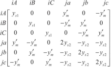
The network topology of the transformer in YN,yn0 connection can be shown as Fig. 7. And its 6 × 6 Y-bus matrix can be given by the matrix operation method as

Ignoring mutual-inductances among the three phases (\(\dot{y} = 0,\ddot{y} = 0,y_{m}^{\prime } = y_{m}\)), the 6 × 6 admittance matrix can be given by

The network topology of the transformer in the Eq. (10) can be shown as Fig. 8.
-
(2)
YN,d11 connection
In Fig. 9, the connected topology of the transformer in YN,d11 connection is presented. For the transformer in the asymmetric magnetic circuits (such as the transformer in three-phase three-limb cores), the node admittance matrix is full because of the coupling among the windings.

Topology of the three-phase three-limb core transformer; the three-phase three-limb core transformer has asymmetric magnetic circuits. The topology shows the relationship between equivalent reactance and connection of the transformer

Topology of the transformer by ignoring mutual-inductances; Ignoring mutual-inductances (When the magnetic circuits is balanced), Topology of the transformer is showed like this

YN,d11 Connection of the transformer; YN,d11 Connection of the transformer in the coins is showed like this. In primary side, Coin X, Y, Z are connected; and (Coin a & z), (Coin b & x) and (Coin c & y) are connected together in secondary side
The boundary condition is given by the Eq. (4). And the Buses X, Y, Z are grounded. We enable to obtain the 6 × 6 Y-bus matrix by the matrix operation method retaining the three-phase variables, shown as

where
According to different magnetic circuits, the Y-bus model can be given from analyzing the Eq. (11):
-
(1)
Ignoring mutual-inductances among the three phases, the model is able to be seen as the connection by three single-phase transformers assembling. The 6 × 6 admittance matrix can be given as
 (12)
(12)

The network topology of the transformer in the Eq. (12) can be shown as Fig. 10.
-
(2)
Same iron-core magnetic circuit: \(y_{m}^{\prime } = \ddot{y}_{m} = \dot{y}_{m} = y_{m}\); and the admittance matrix can be given by
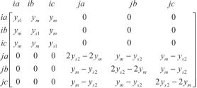 (13)
(13) -
(3)
Plane magnetic circuit layout: \(\dot{y}_{mab} = \dot{y}_{mbc} = \frac{2}{3}y_{m}^{\prime } ,\dot{y}_{mac} = \frac{1}{3}y_{m}^{\prime }\), \(\ddot{y}_{mab} = \ddot{y}_{mbc} = \frac{2}{3}y_{m}^{\prime } ,\ddot{y}_{mac} = \frac{1}{3}y_{m}^{\prime }\); the admittance matrix can be given by
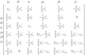 (14)
(14) -
(4)
Three dimensional split magnetic circuit: \(\dot{y}_{mab} = \dot{y}_{mbc} = \dot{y}_{mac} = 0.5y_{m}^{\prime }\), \(\ddot{y}_{mab} = \ddot{y}_{mbc} = \ddot{y}_{mac} = 0.5y_{m}^{\prime }\), and the admittance matrix can be given by
 (15)
(15)


5 Method obtaining the admittances by phase-coordinates
References in this paper attempt to convert directly the parameters of symmetry test into phase-coordinate parameters. In principle, unsymmetrical static three-phase equipment fails to form decoupled 1–2–0 sequence circuits. As a result, the phase-coordinate parameters converted by the decoupled 1–2–0 parameters are approximate values. Compensation method enables to reduce the errors, but it cannot be equivalent. In order to distinguish between nominal values in this section, variables and symbols representing per-unit values are marked “*” in the subscript. In this section, the admittance matrix in the Eq. (6) needs to analyze and calculate.

Topology network of the transformer by ignoring mutual-inductances; Topology network of the transformer by ignoring mutual-inductances is showed in the connection of YN,d11 transformer
5.1 Impedances obtained in the symmetry
Considering the symmetry of structural parameters for three-phase Transformer, the relationship of the Eq. (6) in per-unit system enables to be expressed by
where
\(Z_{P*}\) is the self-admittance on the primary winding;
\(Z_{s*}\) is the self-admittance on the secondary winding;
\(Z_{m*}\) is the mutual-admittance between the primary and the secondary windings at the same iron-core;
\(Z^{\prime}_{m*}\) is the mutual-admittance between the primary windings.
\(Z^{\prime\prime}_{m*}\) is the mutual-admittance between the primary and the secondary windings at the different iron-cores.
\(Z^{\prime\prime\prime}_{m*}\) is the mutual-admittance between the secondary windings.
-
(1)
No-load test: The test enables to obtain the two groups of data, and they are no-load current I0 and no-load loss P0.The relationships of parameters in no-load state can be given by
where
y0* is the no-load admittance; z0* is no-load impedance;
g0* is the no-load conductance;
b0* is the no-load susceptance;
STN is the transformer’s rated capacity.
The no-load impedance can be expressed by
-
(2)
Short circuit test: The test enables to obtain the two groups of data, they are the percentage of short-circuit voltage Vs% and short circuit power loss Pk. The relationships of parameters at short-circuit state can be given by
$$\left\{ {\begin{array}{*{20}l} {R_{T*} = P_{k*} } \\ {\left| {z_{T*} } \right| = V_{s*} } \\ {x_{T*} = \sqrt {\left| {z_{T*} } \right|^{2} - R_{T*}^{2} } } \\ \end{array} } \right.$$(19)where
RT* is the transformer winding resistance; \(\left| {z_{T*} } \right|\) is the leakage reactance; xT* is the winding reactance. And the impedance in short-circuit state can be given by
The Eqs. (10)–(20) deduced under the condition of the symmetrical currents or voltages, the above parameters stand for the positive sequence parameters. The steps for extrapolating the phase-coordinate parameters can be shown as follows:
Considering the same values of leakage reactance on the primary side and secondary side, the relationship (in value system) can be shown by
where
\(Z_{\sigma 1}\),\(Z_{\sigma 2}\) are the leakage reactances on the primary and secondary sides as Fig. 2b shown. The basic parameters in the symmetry in no load test can be given by
The reluctances of transformer’s magnetic circuit are mainly from the air gap between iron cores. According to the principle of magnetic circuit of phase separation test method, there is the relationship shown as follows:
The leakage fluxes run in the air different from those run in the iron-cores. The three-phase symmetrical currents have the effect of magnetization. Similar to three-phase transmission lines, they have the basic relationships of positive sequence impedance and zero sequence impedance. The relationship between positive sequence leakage reactance and phase separation leakage reactance of transformer obtained from short circuit test is as follows:
where
\(x_{\sigma s}\) is self-inductance leakage flux;
\(x_{\sigma m}\) is mutual-inductance leakage flux.
The self-impedance and mutual impedance of the leakage reactance from the short current test can be given by
By substituting the Eqs. (14)–(25), the relationship of the impedance matrix by phase-coordinates in YN,yn0 connection can be given by the modified equation in per-unit system shown as
Figure 11 presents the relationships of the vectors in the parametric systems. The relationships for the parameters in References are shown in Fig. 11a. While the relationships for our modified parameters are shown in Fig. 11b, which enable to explain the work in this section intuitively.

Vector relations in parametric systems; Unmodified parametric system is used to describe vector relations by sequence-coordinates, which only the coupling relationship among windings is considered in (a).While Modified parametric system is used to describe vector relations by phase-coordinates, which coupling relationship among windings is considered containing the tree-phase coupling relations in (b)
5.2 Impedances and admittances obtained in the asymmetry
The magnetic circuits of the three-phase three-limb core transformer can be shown in Fig. 12. The branch Eq. (6) enables to express the relationships of the transformer conveniently.

Magnetic circuits of the three-phase three-limb core transformer; Magnetic circuits of the three-phase three-limb core transformer is showed when The current IA0 is bring to bear on A-phase winding in primary side
Considering the relations of the linear circuits without magnetic saturation, the impedance parameters in the Eq. (6) can be obtained by the open circuit test. Figure 13 shows the coupling relations between the primary side and the secondary side.
-
(1)
At wye side for the open circuit test, when the voltage \(V_{AX} = V_{N}\)(where VN stand for the rated voltage) is applied at the winding “AX”, and the rest windings in opening. We enable to obtain test data for the Eq. (6) shown as
$$\left[ {\begin{array}{*{20}l} {V_{AX}^{0} = V_{N} } \\ {V_{BY}^{0} } \\ {V_{CZ}^{0} } \\ {V_{ax}^{0} } \\ {V_{by}^{0} } \\ {V_{cz}^{0} } \\ \end{array} } \right] = \left[ {\begin{array}{*{20}l} {z_{AA} } & {z_{AB} } & {z_{AC} } & {z_{Aa} } & {z_{Ab} } & {z_{Ac} } \\ {z_{BA} } & {z_{BB} } & {z_{BC} } & {z_{Ba} } & {z_{Bb} } & {z_{Bc} } \\ {z_{CA} } & {z_{CB} } & {z_{CC} } & {z_{Ca} } & {z_{Cb} } & {z_{Cc} } \\ {z_{aA} } & {z_{aB} } & {z_{aC} } & {z_{aa} } & {z_{ab} } & {z_{ac} } \\ {z_{bA} } & {z_{bB} } & {z_{bC} } & {z_{ba} } & {z_{bb} } & {z_{bc} } \\ {z_{cA} } & {z_{cB} } & {z_{cC} } & {z_{ca} } & {z_{cb} } & {z_{cc} } \\ \end{array} } \right]\left[ {\begin{array}{*{20}l} {I_{A0} } \\ 0 \\ 0 \\ 0 \\ 0 \\ 0 \\ \end{array} } \right]$$(27)
where
\(V_{AX}^{0} ,V_{BY}^{0} ,V_{CZ}^{0} ,V_{ax}^{0} ,V_{by}^{0} ,V_{cz}^{0}\) are the testing voltages;
\(I_{A0}^{0}\) is the testing current.

Coupling relations between the primary side and the secondary side by phase-coordinates; Vector graph of the relationship between voltage and coupling is used to describe the Coupling relations between the primary side and the secondary side by phase-coordinates
We can obtain the impedances by per-unit system from the Eq. (20) expressed as
The rest impedances can be obtained by repeating the test two more again.
-
(2)
At delta side for the open circuit test, when the voltage \(V_{ax} = V_{NII}\) (where VNII stands for the rated voltage at the delta side) is applied at the winding “ax”, and the rest windings in opening. We enable to obtain test data for the Eq. (6) shown as
$$\left[ {\begin{array}{*{20}l} {V_{AX}^{d0} } \\ {V_{BY}^{d0} } \\ {V_{CZ}^{d0} } \\ {V_{ax}^{d0} = V_{NII} } \\ {V_{by}^{d0} } \\ {V_{cz}^{d0} } \\ \end{array} } \right] = \left[ {\begin{array}{*{20}l} {z_{AA} } & {z_{AB} } & {z_{AC} } & {z_{Aa} } & {z_{Ab} } & {z_{Ac} } \\ {z_{BA} } & {z_{BB} } & {z_{BC} } & {z_{Ba} } & {z_{Bb} } & {z_{Bc} } \\ {z_{CA} } & {z_{CB} } & {z_{CC} } & {z_{Ca} } & {z_{Cb} } & {z_{Cc} } \\ {z_{aA} } & {z_{aB} } & {z_{aC} } & {z_{aa} } & {z_{ab} } & {z_{ac} } \\ {z_{bA} } & {z_{bB} } & {z_{bC} } & {z_{ba} } & {z_{bb} } & {z_{bc} } \\ {z_{cA} } & {z_{cB} } & {z_{cC} } & {z_{ca} } & {z_{cb} } & {z_{cc} } \\ \end{array} } \right]\left[ {\begin{array}{*{20}l} 0 \\ 0 \\ 0 \\ {I_{a0}^{d} } \\ 0 \\ 0 \\ \end{array} } \right]$$(29)
where
\(V_{AX}^{d0} ,V_{BY}^{d0} ,V_{CZ}^{d0} ,V_{ax}^{d0} ,V_{by}^{d0} ,V_{cz}^{d0}\) are the testing voltages;
\(I_{a0}^{d0}\) is the testing current. And the impedances in per-unit system from the Eq. (22) can be expressed as
The rest impedances can be obtained by repeating the test two more again. Consequently, the impedance matrix by phase-coordinates (in per-unit system) in the Fig. 13 can be given as
6 Results and discussion
6.1 Results
-
(1)
Test by experiment
There are the transformers given as (Type I: Capacity: 60 k VA, Ratio: 400 V/110 V; Type II: Capacity: 1000 k VA, Ratio: 6300 V/400 V). In the Table 1, the mutual inductance coefficient is inversely proportional to the length of magnetic circuit. Ignore measurement errors, the mutual inductance (reactance) coefficients can be approximated as: a-phase [1 0.66 0.33]; b-phase [0.5 1 0.5]; c-phase [0.33 0.66 1] (shown as Fig. 12).
-
(2)
Simulation calculation
The IEEE 4 node feeder test system network is shown in the Fig. 14. The parameters of the test system are as follows: transformer ratio is 12.47(kV):24.9 (kV), and the parameters of transformer and line present in [13]. The tolerance for calculation is 10−5 for testing. The unbalanced loads in bus 4 of the test system are 1250 kW, 1800 kW, 2375 kW, and the power factors are − 0.85, − 0.9 and − 0.95 respectively (Complex power of load marked as S1).

IEEE 4 feeder test system; IEEE 4 feeder test system consists of four nodes, a generator, a transformer, two lines and a load
There are 6 types and parameters of the transformers for testing by power flow calculations. Table 2 presents the types and the parameters of the transformers. In Table 2, The admittance matrix in No. 1 and No. 2 groups of the transformers employ the method in [8] and [12]. And the rest of the transformers use the method in this paper. Table 3 lists the results of power flow calculation for the transformers in D,yn1 connection. And Table 4 presents the results of power flow calculation for the transformers in YN,yn0 connection. Table 5 lists the power flow results for the different power supply in the transformer in YN,yn0 connection.
6.2 Discussion
The calculated results of No. 1 groups at Tables 3 and 4 are the same as [13].Comparing with the results in No. 1 groups of Tables 3 and 4, The results of No. 2 groups are merely smaller, but less errors considering no-load parameters. While both the admittance matrix parameters in the two groups of transformers are calculated by the method in [8] and [12], which the parameters essentially are the positive sequence ones. The method employed in Sect. 5 of this paper is used to calculate the three-phase admittance matrix parameters, and the experiments also show the differences in the test. Comparing with the previously results, the results in No. 3 group and No. 4 group at Tables 3 and 4 are a little smaller and closer in the same condition. Analysis from the physical definition, the true phase admittances are different from the positive sequence ones due to the demagnetization by three-phase symmetrical currents. And the results of different magnetic circuits are given in Tables 3 and 4 as well. Those results also are different from each other.
In Table 5, comparing with the No. 1 group, c-phase voltages are increasing gradually by the changes of loads in No. 6 group, due to the increased unbalances of loads’ currents. Comparing with symmetric component parameters, the effect of node voltages is more different by the phase-coordinates parameters.
Consequently, the three-phase symmetrical currents have the demagnetization, which make the phase-impedances slightly smaller than the synthetic impedances (positive sequence impedance). In addition, the mutual-impedances effect significantly by asymmetry.
7 Conclusions
In this paper, the authors propose the phase-coordinate modeling method by a 12 × 12 primitive full admittance matrix to structure the 6 × 6 admittance matrix (7 × 7 matrix by retention of 1 neutral point) for three-phase transformers in different connections from asymmetric magnetic circuits by the matrix operation method. The phase-coordinate impedances have been corrected by considering the magnetization of three-phase symmetrical currents. There are the advantages shown as follows:
-
Modeling the transformers in different connections and asymmetric magnetic circuits;
-
Real phase-coordinates parameters, which enable calculations accurately.
Finally, the matrix operation method also enables to use for modeling three-phase three-winding transformers usefully, besides the three-phase double-winding transformers. And the method applies to model the non-standard transformers as well.
Availability of data and materials
Data sharing is not applicable to this article as no datasets were generated or analyzed during the current study.
References
Y. Zhu, K. Tomsovic, Adaptive power flow method for distribution systems with dispersed generation. IEEE Trans. Power Delivery 17(3), 822–915 (2002)
M.J.E. Alam, K.M. Muttaqi, D. Sutanto, A three-phase power flow approach for integrated 3-wire MV and 4-wire multigrounded LV networks with rooftop solar PV. IEEE Trans. Power Syst. 17(4), 1238–1244 (2002)
Z. Wang, F. Chen, J. Li, Implementing transformer nodal admittance matrices into backward/forward sweep-based power flow analysis for unbalanced radial distribution system. IEEE Trans. Power Syst. 19(4), 1831–1836 (2004)
M.A. Laughton, Analysis of unbalanced polyphase networks by the method of phase coordinates. Part 1: phase coordinates. Proc. IEE 8(115), 1163–1172 (1968)
T.H. Chen, W.C. Yang, T.Y. Guo, G.C. Pu, Modelling and analysis of asymmetrical three-phase distribution transformer banks with mid-tap connected to the secondary neutral conductor. Electric Power Syst. Res. 19(54), 83–89 (2000)
T. Alinjak, I. Pavic, K. Trupinic, Improved three-phase power flow method for calculation of power losses in unbalanced radial distribution network, in 24th International Conference & Exhibition on Electricity Distribution (CIEED), Session 5: Planning of Power Distribution Systems, pp. 12–15, June, 2017.
J.A. Peralta, F. de LeÓn, J. Mahseredjian, Unbalanced multiphase load-flow using a positive-sequence load-flow program. IEEE Trans. Syst. 23(2), 469–476 (2008)
W. Kersting, Distribution Systems Modeling and Analysis (CRC Press, Boca Raton, FL, 2002).
T.H. Chen, M.S. Chen, T. Inoue, P. Kotas, E.A. Chebli, Three-phase co-generator and transformer models for distribution system analysis. IEEE Trans. Power Del. 6(4), 1671–1681 (1991)
W.H. Kersting, W.H. Phillips, W. Carr, A new approach to modeling three-phase transformer connections. IEEE Trans. Ind. Appl. 35(1), 169–175 (1998)
I. Kocar, J.S. Lacroix, Implementation of a modified augmented nodal analysis based transformer model in the backward forward sweep solver. IEEE Trans. Power Syst. 27(2), 663–670 (2012)
M. Coppo, F. Bignucolo, R. Turri, Generalized transformer modeling for power flow calculation in multi-phase unbalanced networks. IET Gener. Transm. Distrib. 11(4), 3843–3852 (2017)
W.H. Kersting, Radial distribution test feeders. IEEE Trans. Power Syst. 6(3), 975–985 (1991)
Acknowledgements
Not applicable.
Funding
Not applicable. There is no any funding for our research in the paper.
Author information
Authors and Affiliations
Contributions
ZZ finished the algorithm. MM put forward the idea of this paper and English writing of the paper. CW finished the experiments. All authors read and approved the final manuscript.
Corresponding author
Ethics declarations
Competing interests
The authors declare that they have no competing interests.
Additional information
Publisher's Note
Springer Nature remains neutral with regard to jurisdictional claims in published maps and institutional affiliations.
Rights and permissions
Open Access This article is licensed under a Creative Commons Attribution 4.0 International License, which permits use, sharing, adaptation, distribution and reproduction in any medium or format, as long as you give appropriate credit to the original author(s) and the source, provide a link to the Creative Commons licence, and indicate if changes were made. The images or other third party material in this article are included in the article's Creative Commons licence, unless indicated otherwise in a credit line to the material. If material is not included in the article's Creative Commons licence and your intended use is not permitted by statutory regulation or exceeds the permitted use, you will need to obtain permission directly from the copyright holder. To view a copy of this licence, visit http://creativecommons.org/licenses/by/4.0/.
About this article

Cite this article
Zhang, Z., Mo, M. & Wu, C. Three-phase distribution transformer connections modeling based on matrix operation method by phase-coordinates. J Wireless Com Network 2021, 66 (2021). https://doi.org/10.1186/s13638-021-01945-z
Received:
Accepted:
Published:
DOI: https://doi.org/10.1186/s13638-021-01945-z