Dynamics of a stochastic population model with predation effects in polluted environments

Abstract

The present paper puts forward and probes a stochastic single-species model with predation effect in a polluted environment. We propose a threshold between extermination and weak persistence of the species and provide sufficient conditions for the stochastic persistence of the species. In addition, we evaluate the growth rates of the solution. Theoretical findings are expounded by some numerical simulations.

1 Introduction

Environmental pollution because of industry, commerce, agriculture, and the rapid growth of human population has been increasingly prominent and has become an global problem. Pollutants have threatened the health of living organisms. For instance, Amoco Cadiz incident carried off more than 260 thousands tonnes of sea animals in one month [1]; Bhopal disaster killed about 15 thousands people and injured about 560 thousands people [2]; according to the United States Fish and Wildlife Service, pesticides carried off more than 72 million birds every year in US [3].

To probe the influence of pollutants on the evolution of populations, many mathematical models have been put forward. In the 1980s, Hallam and his co-workers [4–6] first constructed a series of deterministic models with pollution and uncovered that environmental pollution has serious influence on the persistence and extermination of the species. These results were improved and extended [7–17]. Particularly, motivated by the fact that the evolution of populations often encounters environmental perturbations [18], several authors (see, e.g., [9, 12–17]) paid attention to stochastic population models with pollution and uncovered that environmental perturbations have vital functions on the persistence and extermination of the species.

On the other hand, most populations have parasites and predators [19]. In general, these predation effects have negative functions on the growth of populations. Therefore we need to test population models with predation effects in polluted environments. However, little research has been conducted to exploit this problem (even for deterministic models).

The objective of this paper is testing the above problem. We construct a population model with predation effects in polluted environments in Sect. 2 and testify that the model has a unique global positive solution in Sect. 3. Then we offer a threshold between extermination and weak persistence of the species and provide conditions under which the species is stochastically persistent in Sect. 4. In Sect. 5, we estimate the growth rates of the solution of the model. Finally, we give the conclusions of this paper and numerically expound the theoretical findings in Sect. 6.

2 The model

Without pollution and predation effects, suppose that the growth of the species follows the logistic role:

$$ \frac{\mathrm{d}\Phi (t)}{\mathrm{d}t}=\Phi (t)\bigl[b-\xi \Phi (t)\bigr], $$

(1)

where $\Phi (t)$ is the population size at time t, and $b>0$ and $\xi >0$ stand for the growth rate and the intraspecific competition rate, respectively.

We consider the predation effects. In general, the predation effects saturate at high prey density and vanish quadratically as the prey density tends to zero [19]. Therefore it is reasonable to model the predation effects by the following function:

$$ \frac{\lambda \Phi ^{2}(t)}{\rho ^{2}+ \Phi ^{2}(t)}, $$

where λ is the upper limit of the predation effects, and $\rho ^{2}$ measures the saturate effect. Then model (1) is replaced by

$$ \frac{\mathrm{d}\Phi (t)}{\mathrm{d}t}=\Phi (t)\bigl[b-\xi \Phi (t)\bigr]- \frac{\lambda \Phi ^{2}(t)}{\rho ^{2}+ \Phi ^{2}(t)}. $$

(2)

As said before, the evolution of populations often encounters environmental perturbations [18]. In general, we can take advantage of a color noise process to portray the environmental perturbations [20], and it is suitable to utilize a Gaussian white noise process to depict a weakly correlated color noise [21]. Various ways were developed to incorporate the white noise into deterministic population models. A widely accepted way is to suppose that some parameters in the model are influenced by the white noise (see, e.g., [22–32]). Adopting these approaches,

$$ b\rightarrow b+\beta _{1}\dot{\psi }_{1}(t),\qquad -\xi \rightarrow -\xi + \beta _{2}\dot{\psi }_{2}(t),\qquad -\lambda \rightarrow \lambda +\beta _{3} \dot{\psi }_{3}(t), $$

where $\psi _{1}(t)$, $\psi _{2}(t)$, and $\psi _{3}(t)$ are independent standard Wiener processes defined on a certain complete probability space $(\Omega,\mathcal{F},\{\mathcal{F}_{t}\}_{t\geq 0},\mathrm{P})$, and $\beta _{i}$, $i=1,2,3$, stand for the intensities. As a result, model (2) is replaced by

$$ \begin{aligned} \mathrm{d} \Phi (t) ={}& \Phi (t) \biggl(b- \xi \Phi (t) - \frac{\lambda \Phi (t)}{\rho ^{2}+ \Phi ^{2}(t)} \biggr){\,\mathrm{d}t} \\ &{}+\beta _{1} \Phi (t)\,\mathrm{d}\psi _{1}(t)+ \beta _{2} \Phi ^{2}(t)\,\mathrm{d}\psi _{2}(t) + \frac{\beta _{3} \Phi ^{2}(t)}{\rho ^{2}+ \Phi ^{2}(t)}\,\mathrm{d} \psi _{3}(t).\end{aligned} $$

(3)

To characterize the influence of pollution, we hypothesize that the populations suck up the pollutants into their bodies [4–6]. Denote by $T(t)$ the concentration of pollutants in the species, which can lead to a descent of the growth rate [4]:

$$ b\rightarrow b-H_{1}\bigl(T(t)\bigr), $$

where $H_{1}(T)$ is a positive continuous increasing function of T. Accordingly, model (3) is replaced by

$$ \begin{aligned} \mathrm{d} \Phi (t) ={}& \Phi (t) \biggl(b-H_{1}\bigl(T(t)\bigr)-\xi \Phi (t) -\frac{\lambda \Phi (t)}{\rho ^{2}+ \Phi ^{2}(t)} \biggr){ \,\mathrm{d}t} \\ &{}+\beta _{1} \Phi (t)\,\mathrm{d}\psi _{1}(t)+ \beta _{2} \Phi ^{2}(t)\,\mathrm{d}\psi _{2}(t) + \frac{\beta _{3} \Phi ^{2}(t)}{\rho ^{2}+ \Phi ^{2}(t)}\,\mathrm{d} \psi _{3}(t).\end{aligned} $$

(4)

To depict the pollutants in the species, we pay attention to the following equation:

$$ \frac{\mathrm{d}T(t)}{\mathrm{d}t}=H_{2}\bigl(T_{e}(t) \bigr)-H_{3}\bigl(T(t)\bigr), $$

(5)

where $T_{e}(t)$ represents the concentration of pollutants in the environment, $H_{2}(T_{e}(t))>0$ characterizes the suck up of pollutants from the environment, $H_{3}(T(t))>0$ measures the loss of pollutants because of excretion and detoxication. Both $H_{2}\in C^{1}$ and $H_{3}\in C^{1}$ are increasing functions.

Finally, we portray the changes of $T_{e}(t)$. Denote by $u(t)$ a continuous and bounded function of t, the input of pollutants from the outside of the environment. Suppose that the changes of $T_{e}(t)$ are governed by the following equation:

$$ \frac{\mathrm{d}T_{e}(t)}{\mathrm{d}t}=u(t)-H_{4}\bigl(T_{e}(t) \bigr), $$

(6)

where $H_{4}\in C^{1}$, measuring the loss of the pollutants from the environment, is an increasing positive function of $T_{e}$.

According to (4)–(6), we derive the following model:

$$ \textstyle\begin{cases} \mathrm{d} \Phi (t) = \Phi (t) (b-H_{1}(T(t))- \xi \Phi (t) -\frac{\lambda \Phi (t)}{\rho ^{2}+ \Phi ^{2}(t)} ){ \,\mathrm{d}t} \\ \phantom{\mathrm{d} \Phi (t) =}{} +\beta _{1} \Phi (t)\,\mathrm{d}\psi _{1}(t)+ \beta _{2} \Phi ^{2}(t)\,\mathrm{d}\psi _{2}(t) + \frac{\beta _{3} \Phi ^{2}(t)}{\rho ^{2}+ \Phi ^{2}(t)}\,\mathrm{d} \psi _{3}(t), \\ \frac{\mathrm{d}T(t)}{\mathrm{d}t}=H_{2}(T_{e}(t))-H_{3}(T(t)), \\ \frac{\mathrm{d}T_{e}(t)}{\mathrm{d}t}=u(t)-H_{4}(T_{e}(t)). \end{cases} $$

(7)

The objectives of this paper is probing some dynamical properties of $\Phi (t)$. Note that the last two equations in model (7) do not depend on $\Phi (t)$, and they have a unique solution $(T(t), T_{e}(t))$ for certain initial value. As a result, from now on we concentrate on Eq. (4).

3 The existence and uniqueness of the solution

Theorem 1

For any initial value $\Phi (0)>0$, Eq. (4) possesses a unique global positive solution $\Phi (t)$ almost surely (a.s.).

Proof

We first concentrate on the equation

$$ \begin{aligned} \mathrm{d}x(t) ={}& \biggl[b-H_{1} \bigl(T(t)\bigr)- \frac{\beta _{1}^{2}}{2}-\xi e^{x(t)} - \frac{\lambda e^{x(t)}}{\rho ^{2}+e^{2x(t)}} - \frac{\beta _{2}^{2}}{2}e^{2x(t)} - \frac{\beta _{3}^{2}e^{2x(t)}}{2(\rho ^{2}+e^{2x(t)})^{2}} \biggr]{ \,\mathrm{d}t} \\ &{} +\beta _{1}\,\mathrm{d}\psi _{1}(t)+\beta _{2}e^{x(t)} \,\mathrm{d}\psi _{2}(t) + \frac{\beta _{3}e^{x(t)}}{\rho ^{2}+e^{2x(t)}}\,\mathrm{d}\psi _{3}(t) \end{aligned} $$

(8)

with $x(0)=\ln \Phi (0)$. By the locally Lipschitz continuity of the coefficients in Eq. (8) we deduce that Eq. (8) possesses a unique solution on $[0,\tau _{e})$, where $\tau _{e}\leq +\infty$. It then follows from Itô’s formula (see [33], p. 32, Theorem 6.2) that $\Phi (t)=e^{x(t)}$ is the unique positive solution of (4).

Now we testify that $\tau _{e}=+\infty$. Let $m_{0}$ be a positive constant such that $m_{0}>\Phi (0)$. For each integer m, define

$$ \tau _{m}=\inf \bigl\{ t\in [0,\tau _{e}): \Phi (t)\geq m \bigr\} . $$

Let $\tau _{\infty }=\lim_{m\rightarrow +\infty }\tau _{m}$. We can deduce that $\tau _{\infty }\leq \tau _{e}$. If $\tau _{e}<+\infty$, then we can find out constants $\hat{T}>0$ and $\epsilon \in (0,1)$ such that

$$ \mathrm{P}\{\tau _{\infty }\leq \hat{T}\}>\epsilon. $$

It then follows that we can find out an integer $m_{1}\geq m_{0}$ such that for any $m\geq m_{1}$,

$$ \mathrm{P}\{\Omega _{m}\}\geq \epsilon, $$

(9)

where $\Omega _{m}=\{\omega:\tau _{m}\leq \hat{T}\}$. Define

$$ W_{1}(\Phi )=\Phi ^{\gamma },\quad \Phi >0, 0< \gamma < 1. $$

Then we deduce by Itô’s formula that

$$ \begin{aligned} &\mathrm{d}W_{1}(\Phi ) \\ & \quad=\gamma \Phi ^{\gamma } \biggl[b-H_{1}\bigl(T(t)\bigr)-\xi \Phi - \frac{\lambda \Phi }{\rho ^{2}+\Phi ^{2}}+ \frac{\gamma -1}{2} \beta _{1}^{2}+ \frac{\gamma -1}{2}\beta _{2}^{2} \Phi ^{2}+ \frac{(\gamma -1)\beta _{3}^{2} \Phi ^{2}}{2(\rho ^{2}+\Phi ^{2})^{2}} \biggr]\,\mathrm{d}t \\ &\qquad{} +\gamma \beta _{1} \Phi ^{\gamma }\,\mathrm{d}\psi _{1}(t)+ \gamma \beta _{2} \Phi ^{\gamma +1} \,\mathrm{d} \psi _{2}(t)+ \frac{\gamma \beta _{3} \Phi ^{\gamma +1} }{\rho ^{2}+\Phi ^{2}} \,\mathrm{d}\psi _{3}(t) \\ &\quad \leq \gamma b W_{1}(\Phi )\,\mathrm{d}t+\gamma W_{1}( \Phi ) \biggl[\beta _{1} \,\mathrm{d}\psi _{1}(t)+\beta _{2} \Phi \,\mathrm{d}\psi _{2}(t)+\frac{\beta _{3}\Phi }{\rho ^{2}+\Phi ^{2}} \, \mathrm{d}\psi _{3}(t) \biggr]. \end{aligned} $$

Accordingly,

$$ \begin{aligned} \mathbb{E}W_{1}\bigl(\Phi (\tau _{m}\wedge \hat{T})\bigr)&\leq W_{1}\bigl( \Phi (0)\bigr)+ \gamma b \int _{0}^{\tau _{m}\wedge \hat{T}}\mathbb{E}W_{1}\bigl( \Phi (s)\bigr)\,\mathrm{d}s \\ &\leq W_{1}\bigl(\Phi (0)\bigr)+\gamma b \int _{0}^{\hat{T}} \mathbb{E}W_{1}\bigl(\Phi ( \tau _{m}\wedge s)\bigr)\,\mathrm{d}s. \end{aligned} $$

By Gronwall’s inequality (see [33], p. 45, Theorem 8.1) we get

$$ \mathbb{E}W_{1}\bigl(\Phi (\tau _{m}\wedge \hat{T})\bigr)\leq W_{1}\bigl(\Phi (0)\bigr)e^{ \gamma b \hat{T}}.$$

(10)

For $\omega \in \Omega _{m}$, $W_{1}(\Phi (\tau _{m},\omega ))\geq m^{\gamma }$. Then by (9) and (10) we can see that

$$ W_{1}\bigl(\Phi (0)\bigr)e^{\gamma b\hat{T}}\geq \mathbb{E} \bigl[1_{\Omega _{m}}( \omega )W_{1}(\Phi (\tau _{m},\omega )\bigr]\geq \epsilon m^{\gamma }. $$

Letting $m\rightarrow +\infty$ gives

$$ W_{1}\bigl(\Phi (0)\bigr)e^{\gamma b\hat{T}}= \infty.$$

(11)

However, by the definitions of $W_{1}(\Phi )$ and T̂ we have

$$ W_{1}\bigl(\Phi (0)\bigr)e^{\gamma b\hat{T}}< +\infty, $$

which is a contradiction with (11). Thereby, $\tau _{e}=+\infty$. □

4 Extinction and persistence

Theorem 2

If $\Lambda <0$, then $\lim_{t\rightarrow +\infty } \Phi (t)=0$ a.s., that is, the species is extinct, where

$$ \Lambda =\Lambda _{1}-\liminf_{t\rightarrow +\infty }t^{-1} \int _{0}^{t} H_{1}\bigl(T(s)\bigr)\, \mathrm{d}s,\quad \Lambda _{1}=b-\frac{1}{2} \beta _{1}^{2}. $$

Proof

We can deduce from Itô’s formula that

$$ \begin{aligned} \mathrm{d}\ln \Phi = {}&\biggl[\Lambda _{1}-H_{1}\bigl(T(t)\bigr)- \xi \Phi -\frac{\lambda \Phi }{\rho ^{2} + \Phi ^{2}}- \frac{\beta _{2}^{2} }{2} \Phi ^{2} - \frac{\beta _{3}^{2} \Phi ^{2}}{2(\rho ^{2} +\Phi ^{2})^{2}} \biggr]{ \,\mathrm{d}t} \\ &{} +\beta _{1} \,\mathrm{d}\psi _{1}(t)+\beta _{2} \Phi \,\mathrm{d}\psi _{2}(t)+\frac{\beta _{3}\Phi }{\rho ^{2} + \Phi ^{2}} \,\mathrm{d}\psi _{3}(t), \end{aligned} $$

that is,

$$ \begin{aligned}& \ln \Phi (t)-\ln \Phi (0)\\ &\quad =\Lambda _{1} t- \int _{0}^{t}H_{1}\bigl(T(s)\bigr) \, \mathrm{d}s \\ &\qquad{}- \int _{0}^{t} \biggl[\xi \Phi (s)+ \frac{\lambda \Phi (s)}{\rho ^{2} + \Phi ^{2}(s)} + \frac{\beta _{2}^{2} }{2} \Phi ^{2}(s)+ \frac{\beta _{3}^{2} \Phi ^{2}(s)}{2(\rho ^{2} + \Phi ^{2}(s))^{2}} \biggr]\,\mathrm{d}s \\ &\qquad{} +\Gamma _{1}(t)+\Gamma _{2}(t)+\Gamma _{3}(t), \end{aligned} $$

(12)

where

$$ \Gamma _{1}(t)=\beta _{1} \psi _{1}(t),\qquad \Gamma _{2}(t)= \int _{0}^{t} \beta _{2} \Phi (s)\, \mathrm{d}\psi _{2}(s),\qquad \Gamma _{3}(t)= \int _{0}^{t} \frac{\beta _{3} \Phi (s)}{\rho ^{2} + \Phi ^{2}(s)}\,\mathrm{d}\psi _{3}(s). $$

The quadratic variations of $\Gamma _{2}(t)$ and $\Gamma _{3}(t)$ are

$$ \bigl\langle \Gamma _{2}(t),\Gamma _{2}(t)\bigr\rangle = \int _{0}^{t}\beta _{2}^{2} \Phi ^{2}(s)\,\mathrm{d}s $$

and

$$ \bigl\langle \Gamma _{3}(t),\Gamma _{3}(t)\bigr\rangle = \int _{0}^{t} \frac{\beta _{3}^{2} \Phi ^{2}(s)}{(\rho ^{2} + \Phi ^{2}(s))^{2}} \,\mathrm{d}s\leq \frac{\beta _{3}^{2}}{2\rho ^{2}} t, $$

respectively. We can easily obtain that

$$ \lim_{t\rightarrow +\infty }t^{-1}\Gamma _{i}(t)=0 \quad\text{a.s., } i=1,3. $$

(13)

By the exponential martingale inequality (see [33], p. 44, Theorem 7.4) we deduce that

$$ \mathrm{P} \biggl\{ \sup_{0\leq t\leq M} \biggl[\Gamma _{2}(t)- \frac{1}{2}\bigl\langle \Gamma _{2}(t),\Gamma _{2}(t) \bigr\rangle \biggr]>2\ln M \biggr\} \leq 1/M^{2}. $$

By the Borel–Cantelli lemma (see [33], p. 7, Lemma 2.4), for almost all $\omega \in \Omega$, there exists an integer $M_{0}=M_{0}(\omega )$ such that for $M\geq M_{0}$,

$$ \sup_{0\leq t\leq M} \biggl[\Gamma _{2}(t)-\frac{1}{2} \bigl\langle \Gamma _{2}(t), \Gamma _{2}(t)\bigr\rangle \biggr]\leq 2\ln M. $$

Therefore, for any $0\leq t\leq M, M\geq M_{0}$,

$$ \Gamma _{2}(t)\leq 2\ln M+\frac{1}{2}\bigl\langle \Gamma _{2}(t),\Gamma _{2}(t) \bigr\rangle =2\ln M+ 0.5 \int _{0}^{t}\beta _{2}^{2} \Phi ^{2}(s) \,\mathrm{d}s.$$

(14)

Then we deduce from (12) and (14) that for any $0\leq t\leq M, M\geq M_{0}$,

$$ \ln \Phi (t)-\ln \Phi (0) \leq \Lambda _{1} t- \int _{0}^{t}H_{1}\bigl(T(s)\bigr) \, \mathrm{d}s -\xi \int _{0}^{t} \Phi (s)\,\mathrm{d}s+2 \ln M+\Gamma _{1}(t)+\Gamma _{3}(t).$$

(15)

For $0< M-1\leq t\leq M, M\geq M_{0}$, we have

$$ t^{-1} \bigl\{ \ln \Phi (t)-\ln \Phi (0) \bigr\} \leq \Lambda _{1}- t^{-1} \int _{0}^{t}H_{1}\bigl(T(s)\bigr)\, \mathrm{d}s+2(M-1)^{-1} \ln M+t^{-1}\Gamma _{1}(t)+t^{-1}\Gamma _{3}(t). $$

Then (13) shows that

$$ \limsup_{t\rightarrow +\infty }t^{-1}\ln \Phi (t)\leq \Lambda _{1}- \liminf_{t\rightarrow +\infty }t^{-1} \int _{0}^{t}H_{1}\bigl(T(s)\bigr) \, \mathrm{d}s=\Lambda < 0. $$

Therefore, for any $\epsilon \in (0,-\Lambda )$, there is $T_{1}$ such that for all $t>T_{1}$,

$$ t^{-1}\ln \Phi (t)\leq \epsilon +\Lambda < 0, $$

That is, for all $t>T_{1}$

$$ \Phi (t)\leq e^{(\epsilon +\Lambda )t}. $$

Hence $\lim_{t\rightarrow +\infty } \Phi (t)=0$ a.s. □

Theorem 3

If $\Lambda \geq 0$, then

$$ \limsup_{t\rightarrow +\infty }t^{-1} \int _{0}^{t} \Phi (s) \,\mathrm{d}s\leq \frac{\Lambda }{\xi }\quad \textit{a.s.}$$

(16)

In particular, $\Lambda =0\Rightarrow$ $\lim_{t\rightarrow +\infty }t^{-1}\int _{0}^{t} \Phi (s) \,\mathrm{d}s=0$, that is, the species is nonpersistent in the mean.

Proof

For arbitrary $\epsilon >0$, we can find $\tilde{T}>0$ such that for $0<\tilde{T}<M-1\leq t\leq M, M\geq M_{0}$,

$$ t^{-1} \biggl[\ln \Phi (0)+\Lambda _{1}- \int _{0}^{t}H_{1}\bigl(T(s)\bigr) \, \mathrm{d}s+2\ln M+\Gamma _{1}(t)+\Gamma _{3}(t) \biggr]\leq \Lambda + \epsilon. $$

Set $\Xi =\Lambda +\epsilon$. In view of (15), for arbitrary $0<\tilde{T}<M-1\leq t\leq M, M\geq M_{0}$, we obtain

$$ \begin{aligned} \ln \Phi (t)& \leq \ln \Phi (0)+\Lambda _{1} t- \int _{0}^{t}H_{1}\bigl(T(s)\bigr) \, \mathrm{d}s-\xi \int _{0}^{t} \Phi (s)\,\mathrm{d}s+2\ln M+\Gamma _{1}(t)+ \Gamma _{3}(t) \\ &\leq \Xi t-\xi \int _{0}^{t} \Phi (s)\,\mathrm{d}s.\end{aligned} $$

Set $\alpha (t)=\int _{0}^{t} \Phi (s)\,\mathrm{d}s$. Then we can see that

$$ e^{\xi \alpha (t)}(\mathrm{d}\alpha /\mathrm{d}t)\leq e^{\Xi t},\quad t \geq \tilde{T}. $$

Integrating both sides from T̃ to t, we get

$$ \int _{\tilde{T}}^{t} e^{\xi \alpha (s)}\,\mathrm{d}\alpha (s)\leq \int _{\tilde{T}}^{t} e^{\Xi s} \,\mathrm{d}s. $$

Therefore

$$ e^{\xi \alpha (t)}\leq e^{\xi \alpha (\tilde{T})}+\xi \Xi ^{-1}e^{ \Xi t}- \xi \Xi ^{-1}e^{\Xi \tilde{T}}. $$

Taking logarithms leads to

$$ \alpha (t)\leq (\xi )^{-1}\ln \bigl\{ \xi \Xi ^{-1}e^{\Xi t}+e^{\xi \alpha (\tilde{T})}- \xi \Xi ^{-1}e^{\epsilon \tilde{T}} \bigr\} . $$

As a result,

$$ \limsup_{t\rightarrow +\infty } t^{-1} \int _{0}^{t} \Phi (s)\,\mathrm{d}s\leq \xi ^{-1}\limsup_{t\rightarrow + \infty } \bigl\{ t^{-1}\ln \bigl\{ \xi \Xi ^{-1}e^{\Xi t}+e^{\xi \alpha ( \tilde{T})}-\xi \Xi ^{-1}e^{\Xi \tilde{T}} \bigr\} \bigr\} . $$

It then follows from L’Hospital’s rule that

$$ \limsup_{t\rightarrow +\infty } t^{-1} \int _{0}^{t} \Phi (s)\,\mathrm{d}s\leq \frac{\Xi }{\xi }=\frac{\Lambda +\epsilon }{\xi }. $$

Since ϵ is arbitrary, we get (16). □

Theorem 4

If $\Lambda >0$, then $\limsup_{t\rightarrow +\infty } \Phi (t)>0$, that is, the species is weakly persistent.

Proof

Denote

$$ L= \Bigl\{ \omega:\lim_{t\rightarrow +\infty } \Phi (t,\omega )=0 \Bigr\} . $$

We hypothesize that $\mathrm{P}\{L\}>0$. For arbitrary $\omega \in L$, $\lim_{t\rightarrow +\infty } \Phi (t,\omega )=0$. Therefore, for any $\epsilon \in (0,1)$, there is T such that $\Phi (t,\omega )\leq \epsilon$ for all $t\geq T$. As a result, for sufficiently large t,

$$\begin{aligned} &t^{-1}\bigl[\ln \Phi (t,\omega )-\ln \Phi (0)\bigr]\leq \ln \epsilon /t\leq 0, \\ &\int _{0}^{t}\beta _{2}^{2} \Phi ^{2}(s,\omega )\,\mathrm{d}s= \int _{0}^{T} \beta _{2}^{2} \Phi ^{2}(s,\omega )\,\mathrm{d}s+ \int _{T}^{t}\beta _{2}^{2} \Phi ^{2}(s,\omega )\,\mathrm{d}s\\ &\phantom{\int _{0}^{t}\beta _{2}^{2} \Phi ^{2}(s,\omega )\,\mathrm{d}s}\leq \beta _{2}^{2}M_{1}+ \beta _{2}^{2} \epsilon (t-T)\leq 2\beta _{2}^{2} \epsilon t, \end{aligned}$$

and

$$ \begin{aligned} & \int _{0}^{t} \biggl[\xi \Phi (s,\omega )+ \frac{\lambda \Phi (s,\omega )}{\rho ^{2} + \Phi ^{2}(s,\omega )} + \frac{\beta _{2}^{2} }{2} \Phi ^{2}(s,\omega )+ \frac{\beta _{3}^{2} \Phi ^{2}(s,\omega )}{2(\rho ^{2} + \Phi ^{2}(s,\omega ))^{2}} \biggr]\,\mathrm{d}s \\ &\quad = \int _{0}^{T} \biggl[\xi \Phi (s,\omega )+ \frac{\lambda \Phi (s,\omega )}{\rho ^{2} + \Phi ^{2}(s,\omega )} + \frac{\beta _{2}^{2} }{2} \Phi ^{2}(s,\omega )+ \frac{\beta _{3}^{2} \Phi ^{2}(s,\omega )}{2(\rho ^{2} + \Phi ^{2}(s,\omega ))^{2}} \biggr]\,\mathrm{d}s \\ &\qquad{} + \int _{T}^{t} \biggl[\xi \Phi (s,\omega )+ \frac{\lambda \Phi (s,\omega )}{\rho ^{2} + \Phi ^{2}(s,\omega )} + \frac{\beta _{2}^{2} }{2} \Phi ^{2}(s,\omega )+ \frac{\beta _{3}^{2} \Phi ^{2}(s,\omega )}{2(\rho ^{2} + \Phi ^{2}(s,\omega ))^{2}} \biggr]\,\mathrm{d}s \\ & \quad\leq M_{2}+ \biggl(\xi +\lambda /\rho ^{2}+ \frac{\beta _{2}^{2} }{2}\epsilon +\frac{\beta _{3}^{2}}{2\rho ^{4}} \epsilon \biggr)\epsilon (t-T) \\ &\quad \leq 2 \biggl(\xi +\lambda /\rho ^{2}+ \frac{\beta _{2}^{2} }{2}+ \frac{\beta _{3}^{2}}{2\rho ^{4}} \biggr) \epsilon t,\end{aligned} $$

where $M_{1}$ and $M_{2}$ are positive constants. Consequently,

$$\begin{aligned} &\limsup_{t\rightarrow +\infty }t^{-1}\bigl[\ln \Phi (t,\omega )- \ln \Phi (0)\bigr]\leq 0, \qquad\lim_{t\rightarrow +\infty }t^{-1} \int _{0}^{t} \beta _{2} \Phi (s,\omega ) \,\mathrm{d}\psi _{2}(s)=0, \\ &\lim_{t\rightarrow +\infty }t^{-1} \int _{0}^{t} \biggl[\xi \Phi (s,\omega )+ \frac{\lambda \Phi (s,\omega )}{\rho ^{2} + \Phi ^{2}(s,\omega )} + \frac{\beta _{2}^{2} }{2} \Phi ^{2}(s,\omega )+ \frac{\beta _{3}^{2} \Phi ^{2}(s,\omega )}{2(\rho ^{2} + \Phi ^{2}(s,\omega ))^{2}} \biggr]\,\mathrm{d}s=0. \end{aligned}$$

We then deduce from (12) and (13) that

$$ 0>\limsup_{t\rightarrow +\infty }t^{-1}\ln \Phi (t,\omega )= \Lambda >0, $$

a contradiction. As a result, $\mathrm{P}\{L\}=0$.

Denote

$$ \widetilde{L}= \Bigl\{ \omega:\limsup_{t\rightarrow +\infty } \Phi (t,\omega )>0 \Bigr\} , $$

and hence $\widetilde{L}\cap L=\emptyset$. Note that $\Phi (t)>0$, and therefore $\widetilde{L}\cup L=\Omega$. Then we deduce from $\mathrm{P}\{L\}=0$ that $\mathrm{P}\{\widetilde{L}\}=1$, which is the required statement. □

Theorems 2–4 uncover that Λ is the threshold between extermination and weak persistence of the species. Now let us test the permanence of the species.

Theorem 5

If $\bar{\Lambda }:=\Lambda _{1}-\limsup_{t\rightarrow +\infty }H_{1}(T(t))>0$, then the species is stochastically permanent, that is, for any $\epsilon \in (0,1)$, we can find two constants $\sigma _{1}=\sigma _{1}(\epsilon )>0$ and $\sigma _{2}=\sigma _{2}(\epsilon )>0$ such that

$$ \liminf_{t\rightarrow +\infty }\mathrm{P} \bigl\{ \Phi (t)\geq \sigma _{1} \bigr\} \geq 1-\epsilon, \qquad\liminf_{t\rightarrow + \infty }\mathrm{P} \bigl\{ \Phi (t)\leq \sigma _{2} \bigr\} \geq 1- \epsilon. $$

Proof

Set

$$ W_{2}(\Phi )=1/ \Phi ^{2},\quad \Phi >0. $$

Then we deduce by Itô’s formula that

$$ \begin{aligned}& \mathrm{d}W_{2}( \Phi )\\ &\quad= 2W_{2}( \Phi ) \biggl[\xi \Phi + \frac{\lambda \Phi }{\rho ^{2} +\Phi ^{2}}-b+H_{1}\bigl(T(t)\bigr) \biggr] \,\mathrm{d}t \\ &\qquad{} +3\beta _{1}^{2} W_{2}( \Phi )\,\mathrm{d}t+3 \beta _{2}^{2} \,\mathrm{d}t + \frac{3\beta _{3}^{2}}{(\rho ^{2} +\Phi ^{2})^{2}}\,\mathrm{d}t \\ &\qquad{} -2\beta _{1} W_{2}( \Phi )\,\mathrm{d}\psi _{1}(t)-2 \beta _{2} \Phi ^{-1}\,\mathrm{d}\psi _{2}(t) - \frac{2\beta _{3} \sqrt{W_{2}( \Phi )}}{\rho ^{2} +\Phi ^{2}} \,\mathrm{d}\psi _{3}(t) \\ &\quad= 2W_{2}( \Phi ) \biggl\{ 1.5\beta _{2}^{2} \Phi ^{2}+\xi \Phi -b+H_{1}\bigl(T(t)\bigr) +1.5\beta _{1}^{2} + \frac{\lambda \Phi }{\rho ^{2} +\Phi ^{2}}+ \frac{1.5\beta _{3}^{2}\Phi ^{2}}{(\rho ^{2} +\Phi ^{2})^{2}} \biggr\} \, \mathrm{d}t \\ &\qquad{} -2\beta _{1} W_{2}( \Phi )\,\mathrm{d}\psi _{1}(t)-2 \beta _{2} \Phi ^{-1}\,\mathrm{d}\psi _{2}(t) - \frac{2\beta _{3} \sqrt{W_{2}( \Phi )}}{\rho ^{2} +\Phi ^{2}} \,\mathrm{d}\psi _{3}(t).\end{aligned} $$

Choose a constant $\varpi \in (0,1)$ that satisfies

$$ \varpi < \bar{\Lambda }/\beta ^{2}_{1}.$$

(17)

Set

$$ W_{3}( \Phi )=\bigl(1+W_{2}( \Phi )\bigr)^{\varpi }. $$

Then we deduce by Itô’s formula that for sufficiently large t,

$$ \mathbb{E}W_{3}\bigl( \Phi (t)\bigr)=W_{3}\bigl( \Phi (0) \bigr)+\mathbb{E} \int _{0}^{t} \mathcal{L}W_{3}\bigl( \Phi (s)\bigr)\,\mathrm{d}s, $$

where

$$\begin{aligned} &\mathcal{L}W_{3}( \Phi ) \\ &\quad= 2\varpi \bigl(1+W_{2}( \Phi )\bigr)^{\varpi -2} \biggl\{ \bigl(W_{2}( \Phi )+W_{2}^{2}( \Phi )\bigr) \biggl[1.5\beta _{2}^{2} \Phi ^{2} +\xi \Phi + \frac{\lambda \Phi }{\rho ^{2} +\Phi ^{2}}\\ &\qquad{}+ \frac{1.5\beta _{3}^{2} \Phi ^{2}}{(\rho ^{2} +\Phi ^{2})^{2}}-b+H_{1}\bigl(T(t)\bigr)+1.5 \beta _{1}^{2} \biggr] \\ &\qquad{} + (\varpi -1)W_{2}^{2}( \Phi )\beta _{1}^{2} +( \varpi -1)W_{2}( \Phi )\beta _{2}^{2} + \frac{(\varpi -1)W_{2}( \Phi )\beta _{3}^{2}}{(\rho ^{2} +\Phi ^{2})^{2}} \biggr\} \\ &\quad=2\varpi \bigl(1+W_{2}( \Phi )\bigr)^{\varpi -2} \biggl\{ \biggl[-b+H_{1}\bigl(T(t)\bigr) +\frac{\beta _{1}^{2} }{2} + \varpi \beta _{1}^{2} \biggr]W_{2}^{2}(\Phi ) \\ &\qquad{}+\xi W_{2}^{1.5}( \Phi ) + \frac{\lambda }{\rho ^{2} +\Phi ^{2}}W_{2}^{1.5}( \Phi ) \\ &\qquad{} + \biggl[-b+H_{1}\bigl(T(t)\bigr) +1.5\beta _{1}^{2} + \frac{\lambda \Phi }{\rho ^{2} +\Phi ^{2}} + \frac{(\varpi +0.5)\beta _{3}^{2}}{(\rho ^{2} +\Phi ^{2})^{2}} +( \varpi +0.5)\beta _{2}^{2} \biggr]W_{2}( \Phi )\\ &\qquad{}+\xi W_{2}^{0.5}( \Phi ) +1.5\beta _{2}^{2} + \frac{1.5\beta _{3}^{2}}{(\rho ^{2} +\Phi ^{2})^{2}} \biggr\} \\ &\quad\leq 2\varpi \bigl(1+W_{2}( \Phi )\bigr)^{\varpi -2} \biggl\{ \Bigl[-\Lambda _{1}+\limsup_{t\rightarrow + \infty }H_{1} \bigl(T(t)\bigr)+\epsilon +\varpi \beta _{1}^{2} \Bigr]W_{2}^{2}( \Phi )\\ &\qquad{}+ \biggl(\xi +\frac{\lambda }{\rho ^{2} } \biggr)W_{2}^{1.5}( \Phi ) \\ &\qquad{} + \biggl[\limsup_{t\rightarrow +\infty }H_{1}\bigl(T(t)\bigr)+ \epsilon +1.5\bigl(\beta _{1}^{2} +\beta _{2}^{2}+ \beta _{3}^{2}/\rho ^{4} \bigr)+ \frac{\lambda }{2\rho } \biggr]W_{2}( \Phi )\\ &\qquad{} +\xi W_{2}^{0.5}( \Phi )+1.5 \beta _{2}^{2}+1.5\beta _{3}^{2}/ \rho ^{4} \biggr\} \\ &\quad=2\varpi \bigl(1+W_{2}(\Phi )\bigr)^{\varpi -2} \biggl\{ - \bigl[ \overline{\Lambda }-\varpi \beta _{1}^{2}- \epsilon \bigr]W_{2}^{2}(a)+ \biggl(\xi +\frac{\lambda }{\rho ^{2} } \biggr)W_{2}^{1.5}( \Phi ) \\ &\qquad{} + \biggl[\limsup_{t\rightarrow +\infty }H_{1}\bigl(T(t)\bigr)+ \epsilon +1.5\bigl(\beta _{1}^{2} +\beta _{2}^{2}+ \beta _{3}^{2}/\rho ^{4} \bigr)+ \frac{\lambda }{2\rho } \biggr]W_{2}( \Phi )\\ &\qquad{}+\xi W_{2}^{0.5}( \Phi )+1.5 \beta _{2}^{2} +1.5\beta _{3}^{2}/ \rho ^{4} \biggr\} . \end{aligned}$$

Here $\epsilon <\bar{\Lambda }-\varpi \beta _{1}^{2}$. Choose a constant $\nu >0$ that satisfies

$$ \overline{\Lambda }-\varpi \beta _{1}^{2}- \epsilon - \frac{\nu }{2\varpi }>0.$$

(18)

Set

$$ W_{4}( \Phi )=e^{\nu t}W_{3}(\Phi ). $$

Then we deduce bymItô’s formula that for sufficiently large t,

$$ \mathbb{E}W_{4}\bigl(\Phi (t)\bigr)=W_{3}\bigl( \Phi (0) \bigr)+\mathbb{E} \int _{0}^{t} \mathcal{L}W_{4}\bigl( \Phi (s)\bigr)\,\mathrm{d}s, $$

where

$$\begin{aligned} \mathcal{L}W_{4}(\Phi )={}&\nu e^{\nu t}\bigl(1+W_{2}(\Phi )\bigr)^{\varpi }+e^{ \nu t} \mathcal{L}W_{3}(\Phi ) \\ \leq{}& 2 e^{\nu t}\varpi \bigl(1+W_{2}( \Phi ) \bigr)^{\varpi -2} \biggl\{ - \biggl[\overline{\Lambda }-\varpi \beta _{1}^{2}- \frac{\nu }{2\varpi }-\epsilon \biggr]W_{2}^{2}( \Phi )\\ &{}+ \biggl(\xi + \frac{\lambda }{\rho ^{2} } \biggr)W_{2}^{1.5}(\Phi ) \\ &{} + \biggl[\limsup_{t\rightarrow +\infty }H_{1}\bigl(T(t)\bigr)+ \epsilon +1.5\bigl(\beta _{1}^{2} +\beta _{2}^{2}+ \beta _{3}^{2} /\rho ^{4} \bigr)+ \frac{\lambda }{2\rho }+\frac{\nu }{\varpi } \biggr]W_{2}(\Phi ) \\ &{} +\xi W_{2}^{0.5}(\Phi )+1.5\beta _{2}^{2}+1.5 \beta _{3}^{2}/ \rho ^{4} +\frac{\nu }{2\varpi } \biggr\} \\ =:{}&e^{\nu t}\sigma (\Phi ). \end{aligned}$$

According to (18),

$$ \tilde{\sigma }:= \sup_{\Phi >0}\sigma ( \Phi )< +\infty. $$

Thereby

$$ \mathbb{E}\bigl[e^{\nu t}\bigl(1+W_{2}\bigl(\Phi (t)\bigr) \bigr)^{\varpi }\bigr]\leq \bigl(1+ \Phi ^{-2}(0) \bigr)^{\varpi }+\nu ^{-1}\tilde{\sigma }\bigl(e^{\nu t}-1 \bigr). $$

Accordingly,

$$ \begin{aligned}\limsup_{t\rightarrow +\infty }\mathbb{E}\bigl[ \Phi ^{-2\varpi }(t)\bigr]&= \limsup_{t\rightarrow +\infty }\mathbb{E} \bigl[W_{2}^{\varpi }\bigl(\Phi (t)\bigr)\bigr] \\ &\leq \limsup _{t\rightarrow +\infty }\mathbb{E}\bigl[\bigl(1+W_{2}\bigl(\Phi (t) \bigr)\bigr)^{\varpi }\bigr]\leq \tilde{\sigma }.\end{aligned} $$

(19)

For any $\epsilon >0$, set $\sigma _{1}= (\epsilon /\tilde{\sigma } )^{\frac{1}{2\varpi }}$. By Chebyshev’s inequality (see [33], p. 5),

$$ \mathrm{P} \bigl\{ \Phi (t)< \sigma _{1} \bigr\} =\mathrm{P} \bigl\{ \Phi ^{-2 \varpi }(t)>\sigma _{1}^{-2\varpi } \bigr\} \leq \frac{\mathbb{E}[ \Phi ^{-2\varpi }(t)]}{\sigma _{1}^{-2\varpi }}= \sigma _{1}^{2\varpi } \mathbb{E}\bigl[ \Phi ^{-2\varpi }(t)\bigr]. $$

Thereby

$$ \limsup_{t\rightarrow +\infty }\mathrm{P} \bigl\{ \Phi (t)< \sigma _{1} \bigr\} \leq \epsilon. $$

Accordingly,

$$ \liminf_{t\rightarrow +\infty }\mathrm{P} \bigl\{ \Phi (t)\geq \sigma _{1} \bigr\} \geq 1-\epsilon. $$

Now we testify

$$ \liminf_{t\rightarrow +\infty }\mathrm{P} \bigl\{ \Phi (t)\leq \sigma _{2} \bigr\} \geq 1-\epsilon.$$

(20)

Set

$$ W_{5}(\Phi )= \Phi ^{c}, \quad\Phi >0, 0< c< 1. $$

Then we deduce by Itô’s formula that

$$\begin{aligned} &\mathrm{d}\bigl(e^{t}W_{5}( \Phi )\bigr)\\ &\quad =e^{t} \biggl\{ \Phi ^{c}+c \Phi ^{c} \biggl[b -\xi \Phi -\frac{\lambda \Phi }{\rho ^{2} +\Phi ^{2}}+ \frac{c-1}{2}\beta _{1}^{2} +\frac{c-1}{2}\beta _{2}^{2} \Phi ^{2}+ \frac{(c-1)\beta _{3}^{2}\Phi ^{2}}{2(\rho ^{2} +\Phi ^{2})^{2}} \biggr] \biggr\} \,\mathrm{d}t \\ & \qquad{}+c\beta _{1}e^{t}\Phi ^{c}\,\mathrm{d}\psi _{1}(t)+c \beta _{2}e^{t} \Phi ^{ c+1} \, \mathrm{d}\psi _{2}(t)+c \beta _{3} e^{t} \frac{\Phi ^{ c+1}}{\rho ^{2} +\Phi ^{2}}\,\mathrm{d} \psi _{3}(t) \\ &\quad \leq e^{t}\sigma _{3}\,\mathrm{d}t+ c e^{t} \Phi ^{c} \biggl[\beta _{1} \,\mathrm{d}\psi _{1}(t)+\beta _{2}\Phi \,\mathrm{d} \psi _{2}(t)+ \frac{ \beta _{3}\Phi }{\rho ^{2} +\Phi ^{2}}\,\mathrm{d} \psi _{3}(t) \biggr], \end{aligned}$$

where $\sigma _{3}>0$ is a constant. Accordingly,

$$ \limsup_{t\rightarrow +\infty }\mathbb{E}\bigl[ \Phi ^{c}(t)\bigr] \leq \sigma _{3}. $$

By Chebyshev’s inequality we derive (20). □

5 Upper- and lower-growth rates

Theorem 6

For model (4), we have

$$ \limsup_{t\rightarrow +\infty }\frac{\ln \Phi (t)}{\ln t} \leq 1, \quad \textit{a.s.}$$

(21)

Proof

We deduce from Itô’s formula that

$$ \begin{aligned} &\mathrm{d}\bigl[e^{t}\ln \Phi \bigr] \\ &\quad = e^{t} \biggl[ \ln \Phi +b-H_{1}\bigl(T(t)\bigr)- \frac{\beta _{1}^{2} }{2}-\xi \Phi - \frac{\beta _{2}^{2} }{2}\Phi ^{2}- \frac{\lambda \Phi }{\rho ^{2} +\Phi ^{2}}- \frac{\beta _{3}^{2} \Phi ^{2}}{2(\rho ^{2} +\Phi ^{2})^{2}} \biggr]{ \,\mathrm{d}t} \\ &\qquad{} +\beta _{1} e^{t} \,\mathrm{d}\psi _{1}(t)+ \beta _{2} e^{t} \Phi \,\mathrm{d}\psi _{2}(t) + \frac{\beta _{3} e^{t}\Phi }{\rho ^{2} +\Phi ^{2}}\,\mathrm{d}\psi _{3}(t). \end{aligned} $$

Accordingly,

$$ \begin{aligned} &e^{t} \ln \Phi (t)-\ln \Phi (0) \\ &\quad= \int _{0}^{t} e^{s} \biggl[\ln \Phi (s)+b-H_{1}\bigl(T(s)\bigr)-\frac{\beta _{1}^{2} }{2}-\xi \Phi (s)- \frac{\beta _{2}^{2} }{2}\Phi ^{2}(s) - \frac{\lambda \Phi (s)}{\rho ^{2} +\Phi ^{2}(s)} \\ &\qquad{} - \frac{\beta _{3}^{2} \Phi ^{2}(s)}{2(\rho ^{2} +\Phi ^{2}(s))^{2}} \biggr]{\,\mathrm{d}s} +\Gamma _{4}(t)+\Gamma _{5}(t)+\Gamma _{6}(t),\end{aligned} $$

(22)

where

$$\begin{aligned} &\Gamma _{4}(t)= \int _{0}^{t}\beta _{1}e^{s}\, \mathrm{d}\psi _{1}(s),\qquad \Gamma _{5}(t)= \int _{0}^{t}\beta _{2}e^{s} \Phi (s)\,\mathrm{d}\psi _{2}(s), \\ &\Gamma _{6}(t)= \int _{0}^{t} \frac{\beta _{3}e^{s}\Phi (s)}{\rho ^{2} +\Phi ^{2}(s)}\,\mathrm{d} \psi _{3}(s). \end{aligned}$$

Set

$$ \Gamma (t)=\Gamma _{4}(t)+\Gamma _{5}(t)+\Gamma _{6}(t). $$

Thereby

$$ \bigl\langle \Gamma (t),\Gamma (t)\bigr\rangle = \int _{0}^{t} e^{2s} \biggl[\beta _{1}^{2} +\beta _{2}^{2} \Phi ^{2}(s)+ \frac{\beta _{3}^{2} \Phi ^{2}(s)}{(\rho ^{2} +\Phi ^{2}(s))^{2}} \biggr]\,\mathrm{d}s.$$

By the exponential martingale inequality (see [33], p. 44, Theorem 7.4), for any $\kappa >1$ and $\varrho >0$,

$$ \mathrm{P} \biggl\{ \sup_{0\leq t\leq \varrho m} \biggl[\Gamma (t)- \frac{e^{-\varrho m}}{2} \bigl\langle \Gamma (t),\Gamma (t)\bigr\rangle \biggr]> \kappa e^{\varrho m} \ln m \biggr\} \leq m^{-\kappa }. $$

By Borel–Cantelli’s lemma (see [33], p. 7, Lemma 2.4) we deduce that for almost all $\omega \in \Omega$, there is $m_{2}$ such that for any $m\geq m_{2}$,

$$ \Gamma (t)\leq \frac{e^{-\varrho m}}{2} \bigl\langle \Gamma (t),\Gamma (t) \bigr\rangle + e^{\varrho m} \ln m,\quad 0\leq t\leq \varrho m. $$

Accordingly, for $m\geq m_{2}$ and $0\leq t\leq \varrho m$,

$$ \Gamma (t) \leq \frac{e^{-\varrho m}}{2} \int _{0}^{t} e^{2s} \biggl[\beta _{1}^{2} +\beta _{2}^{2} \Phi ^{2}(s)+ \frac{\beta _{3}^{2} \Phi ^{2}(s)}{(\rho ^{2} +\Phi ^{2}(s))^{2}} \biggr]\,\mathrm{d}s+\kappa e^{\varrho m} \ln m.$$

Then from (22) it follows that for $m\geq m_{2}$ and $0\leq t\leq \varrho m$,

$$ \begin{aligned} &e^{t} \ln \Phi (t)-\ln \Phi (0) \\ &\quad\leq \int _{0}^{t} e^{s} \biggl[\ln \Phi (s)+b-H_{1}\bigl(T(s)\bigr) -\frac{\beta _{1}^{2} }{2}-\xi \Phi (s)- \frac{\beta _{2}^{2} }{2} \Phi ^{2}(s)\\ &\qquad{} -\frac{\lambda \Phi (s)}{\rho ^{2} +\Phi ^{2}(s)}- \frac{\beta _{3}^{2}\Phi ^{2}(s))}{2(\rho ^{2} +\Phi ^{2}(s))^{2}} \biggr]{\,\mathrm{d}s} \\ &\qquad{} +\frac{e^{-\varrho m}}{2} \int _{0}^{t} e^{2s} \biggl[\beta _{1}^{2}+\beta _{2}^{2} \Phi ^{2}(s)+ \frac{\beta _{3}^{2} \Phi ^{2}(s))}{(\rho ^{2} +\Phi ^{2}(s))^{2}} \biggr]\,\mathrm{d}s+\kappa e^{\varrho m} \ln m \\ &\quad = \int _{0}^{t} e^{s} \biggl[\ln \Phi (s)+b-H_{1}\bigl(T(s)\bigr) - \xi \Phi (s)\\ &\qquad{}-\frac{1-e^{s-\varrho m}}{2} \biggl( \beta _{1}^{2}+\beta _{2}^{2} \Phi ^{2}(s)+ \frac{\beta _{3}^{2}\Phi ^{2}(s)}{\rho ^{2} +\Phi ^{2}(s))^{2}} \biggr) \biggr]{\,\mathrm{d}s}+\kappa e^{\varrho m} \ln m \\ &\quad \leq \int _{0}^{t} e^{s} \bigl[\ln \Phi (s)+b-\xi \Phi (s) \bigr]{\,\mathrm{d}s}+\kappa e^{\varrho m} \ln m \\ & \quad\leq \sigma _{4}\bigl(e^{t} -1\bigr)+\kappa e^{\varrho m} \ln m,\end{aligned} $$

where $\sigma _{4}=\max \{1,-\ln \xi +b-1\}$. As a result, for $0<\varrho (m-1)\leq t\leq \varrho m$ and $m\geq m_{2}$, we derive

$$ \frac{\ln \Phi (t)}{\ln t}\leq \frac{e^{-t} \ln \Phi (0)}{\ln t}+ \frac{\sigma _{4}(1- e^{-t})}{\ln t}+ \frac{\kappa e^{-\varrho (m-1)} e^{\varrho m}\ln m}{\ln (\varrho (m-1))}. $$

Note that

$$ \lim_{m\rightarrow +\infty }\frac{\ln m}{\ln (\varrho (m-1))} = \lim_{m\rightarrow +\infty } \frac{\ln m}{\ln \varrho +\ln (m-1)}=1. $$

Accordingly,

$$ \limsup_{t\rightarrow +\infty }\frac{\ln \Phi (t)}{\ln t} \leq \kappa e^{\varrho }. $$

Letting $\kappa \rightarrow 1$ and $\varrho \rightarrow 0$, we obtain (21). □

Theorem 6 probes the upper-growth rate of $\Phi (t)$. Now let us consider the lower-growth rate of $\Phi (t)$.

Theorem 7

If $\bar{\Lambda }>0$, then

$$ \liminf_{t\rightarrow +\infty } \frac{\ln \Phi (t)}{\ln t}\geq - \frac{1}{2\varpi }. $$

(23)

Proof

We can deduce from (19) that there is a constant $\sigma _{5}>0$ such that

$$ \mathbb{E} \bigl[ \bigl(1+W_{2}\bigl( \Phi (t)\bigr) \bigr)^{\varpi } \bigr]\leq \sigma _{5},\quad t\geq 0. $$

(24)

By Itô’s formula,

$$ \begin{aligned} &\mathrm{d}\bigl[\bigl(1+W_{2}( \Phi ) \bigr)^{\varpi }\bigr] \\ &\quad =2\varpi \bigl(1+W_{2}( \Phi )\bigr)^{\varpi -2} \biggl\{ \biggl[-b+H_{1}\bigl(T(t)\bigr) +\frac{\beta _{1}^{2}}{2}+ \frac{\lambda \Phi }{\rho ^{2} +\Phi ^{2}}+ \varpi \beta _{1}^{2} \biggr]W_{2}^{2}( \Phi ) \\ &\qquad{} +\xi W_{2}^{1.5}( \Phi )+ \biggl[-b+H_{1} \bigl(T(t)\bigr)+1.5 \beta _{1}^{2} +\frac{\lambda \Phi }{\rho ^{2} +\Phi ^{2}}\\ &\qquad{}+ \frac{(\varpi +1/2)\beta _{3}^{2}}{(\rho ^{2} +\Phi ^{2})^{2}}+( \varpi +1/2)\beta _{2}^{2} \biggr]W_{2}( \Phi ) \\ &\qquad{} +\xi W_{2}^{0.5}( \Phi ) +1.5\beta _{2}^{2}+ \frac{1.5\beta _{3}^{2} }{(\rho ^{2} +\Phi ^{2})^{2}} \biggr\} \\ &\qquad{} -2\varpi \bigl(1+W_{2}( \Phi )\bigr)^{\varpi -1} \biggl[\beta _{1} W_{2}( \Phi )\,\mathrm{d}\psi _{1}(t) +\beta _{2} \Phi ^{-1} \,\mathrm{d}\psi _{2}(t)+ \frac{\beta _{3} \Phi ^{-1}}{\rho ^{2} +\Phi ^{2}}\,\mathrm{d}\psi _{3}(t) \biggr] \\ &\quad \leq 2\varpi \bigl(1+W_{2}( \Phi )\bigr)^{\varpi -2} \bigl\{ \mu _{1} W_{2}^{2}( \Phi )+\mu _{2}W_{2}^{1.5}( \Phi )+\mu _{3}W_{2}( \Phi )+\mu _{2}W_{2}^{0.5}( \Phi )+\mu _{4} \bigr\} \\ &\qquad{} -2\varpi \bigl(1+W_{2}( \Phi )\bigr)^{\varpi -1} \biggl[\beta _{1} W_{2}( \Phi )\,\mathrm{d}\psi _{1}(t) +\beta _{2} \Phi ^{-1} \,\mathrm{d}\psi _{2}(t)+ \frac{\beta _{3} \Phi ^{-1}}{\rho ^{2} +\Phi ^{2}}\,\mathrm{d}\psi _{3}(t) \biggr], \end{aligned} $$

where

$$\begin{aligned} &\mu _{1}=-b+\limsup_{t\rightarrow +\infty }H_{1}\bigl(T(t) \bigr)+ \epsilon + \biggl(\varpi +\frac{1}{2} \biggr)\beta _{1}^{2} + \frac{\lambda }{2\rho },\qquad \mu _{2}=\xi, \\ &\mu _{3}=-b+\limsup_{t\rightarrow +\infty }H_{1}\bigl(T(t) \bigr)+ \epsilon +1.5 \biggl(\beta _{1}^{2} + \frac{\beta _{3}^{2} }{2\rho ^{2} } \biggr)+\frac{\lambda }{2\rho }+ \biggl(\varpi +\frac{1}{2} \biggr)\beta _{2}^{2}, \\ &\mu _{4}=1.5 \biggl\{ \beta _{2}^{2} +\frac{\beta _{3}^{2} }{2\rho ^{2} } \biggr\} . \end{aligned}$$

Choose a positive constant $\sigma _{6}$ such that

$$ 2\varpi \bigl(\mu _{1} W_{2}^{2}( \Phi )+\mu _{2}W_{2}^{1.5}( \Phi )+\mu _{3}W_{2}( \Phi )+\mu _{2}W_{2}^{0.5}( \Phi )+\mu _{4}\bigr)\leq \sigma _{6}\bigl(1+W_{2}( \Phi ) \bigr)^{2}. $$

Accordingly,

$$ \begin{aligned} \mathrm{d}\bigl(\bigl(1+W_{2}( \Phi )\bigr)^{\varpi }\bigr) \leq{}& \sigma _{6} \bigl(1+W_{2}( \Phi )\bigr)^{\varpi }\,\mathrm{d}t-2\varpi \bigl(1+W_{2}( \Phi )\bigr)^{\varpi -1} \\ &{} \times \biggl[\beta _{1} W_{2}(\Phi )\,\mathrm{d}\psi _{1}(t)+ \beta _{2} \Phi ^{-1}\,\mathrm{d}\psi _{2}(t)+ \frac{\beta _{3} \Phi ^{-1}}{\rho ^{2} +\Phi ^{2}}\,\mathrm{d}\psi _{3}(t) \biggr]. \end{aligned} $$

(25)

Choose a positive constant θ such that

$$ \sigma _{6}\theta +12\varpi \theta ^{0.5} \bigl(\beta _{1}+\beta _{2}+ \beta _{3}/\rho ^{2} \bigr)< \frac{1}{2}. $$

(26)

Let $N=1,2,\dots$. Then from (25) we deduce that

$$ \begin{aligned} & \mathbb{E} (\sup_{(N-1)\theta \leq t\leq N\theta } \bigl(1+W_{2}\bigl( \Phi (t)\bigr)^{\varpi } \bigr) \\ &\quad \leq \mathbb{E} \bigl(1+W_{2}\bigl( \Phi \bigl((N-1)\theta \bigr) \bigr) \bigr)^{\varpi }\\ &\qquad{}+ {\sigma _{6}}\mathbb{E} \biggl(\sup _{(N-1)\theta \leq t \leq N\theta } \biggl\vert \int _{(N-1)\theta }^{t} \bigl(1+W_{2}\bigl( \Phi (s)\bigr) \bigr)^{\varpi }\,\mathrm{d}s \biggr\vert \biggr) \\ & \qquad{}+2\varpi \mathbb{E} \biggl(\sup_{(N-1)\theta \leq t \leq N\theta } \biggl\vert \int _{(N-1)\theta }^{t} \bigl(1+W_{2}\bigl( \Phi (s)\bigr) \bigr)^{\varpi -1} \biggl[\beta _{1} W_{2}\bigl( \Phi (s)\bigr)\,\mathrm{d}\psi _{1}(s) \\ &\qquad{} +\beta _{2} \Phi ^{-1}(s)\,\mathrm{d}\psi _{2}(s)+ \frac{\beta _{3} \Phi ^{-1}(s)}{\rho ^{2} +\Phi ^{2}(s)}\,\mathrm{d} \psi _{3}(s) \biggr] \biggr\vert \biggr). \end{aligned} $$

(27)

By the Burkholder–Davis–Gundy inequality (see [33], p. 40, Theorem 7.3) we have

$$ \begin{aligned} & \mathbb{E} \biggl(\sup _{(N-1)\theta \leq t\leq N\theta } \biggl\vert \int _{(N-1)\theta }^{t} \bigl(1+W_{2}\bigl( \Phi (s)\bigr) \bigr)^{\varpi -1} \biggl[\beta _{1} W_{2}\bigl( \Phi (s)\bigr)\,\mathrm{d}\psi _{1}(s) \\ &\qquad{} +\beta _{2} \Phi ^{-1}(s)\,\mathrm{d}\psi _{2}(s)+ \frac{\beta _{3} \Phi ^{-1}(s)}{\rho ^{2} +\Phi ^{2}(s)}\,\mathrm{d} \psi _{3}(s) \biggr] \biggr\vert \biggr) \\ &\quad\leq \mathbb{E} \biggl(\sup_{(N-1)\theta \leq t\leq N \theta } \biggl\vert \int _{(N-1)\theta }^{t} \bigl(1+W_{2}\bigl( \Phi (s)\bigr) \bigr)^{ \varpi -1} \bigl[\beta _{1} W_{2}\bigl( \Phi (s)\bigr) \bigr]\,\mathrm{d}\psi _{1}(s) \biggr\vert \biggr) \\ &\qquad{} +\mathbb{E} \biggl(\sup_{(N-1)\theta \leq t\leq N \theta } \biggl\vert \int _{(N-1)\theta }^{t} \bigl(1+W_{2}\bigl( \Phi (s)\bigr) \bigr)^{ \varpi -1} \bigl[\beta _{2} \Phi ^{-1}(s) \bigr] \,\mathrm{d}\psi _{2}(s) \biggr\vert \biggr) \\ &\qquad{} +\mathbb{E} \biggl(\sup_{(N-1)\theta \leq t\leq N \theta } \biggl\vert \int _{(N-1)\theta }^{t} \bigl(1+W_{2}\bigl( \Phi (s)\bigr) \bigr)^{ \varpi -1} \biggl[ \frac{\beta _{3} \Phi ^{-1}(s)}{\rho ^{2} +\Phi ^{2}(s)} \biggr] \,\mathrm{d} \psi _{3}(s) \biggr\vert \biggr) \\ &\quad\leq 6 \mathbb{E} \biggl( \int _{(N-1)\theta }^{N \theta } \bigl(1+W_{2}\bigl( \Phi (s)\bigr) \bigr)^{2\varpi -2} \bigl[\beta _{1} W_{2}\bigl( \Phi (s)\bigr) \bigr]^{2}\,\mathrm{d}s \biggr)^{0.5} \\ &\qquad{} + 6 \mathbb{E} \biggl( \int _{(N-1)\theta }^{N \theta } \bigl(1+W_{2}\bigl( \Phi (s)\bigr) \bigr)^{2\varpi -2} \bigl[\beta _{2} \Phi ^{-1}(s) \bigr]^{2}\,\mathrm{d}s \biggr)^{0.5} \\ &\qquad{} +6 \mathbb{E} \biggl( \int _{(N-1)\theta }^{N \theta } \bigl(1+W_{2}\bigl( \Phi (s)\bigr) \bigr)^{2\varpi -2} \biggl[ \frac{\beta _{3} }{\rho ^{2} } \Phi ^{-1}(s) \biggr]^{2} \,\mathrm{d}s \biggr)^{0.5} \\ &\quad\leq 6\theta ^{0.5} \bigl[\beta _{1}+\beta _{2}+ \beta _{3}/ \rho ^{2} \bigr]\mathbb{E} \Bigl(\sup _{(N-1)\theta \leq t\leq N\theta } \bigl(1+W_{2}\bigl( \Phi (t)\bigr) \bigr)^{\varpi } \Bigr). \end{aligned} $$

(28)

Moreover,

$$ \begin{aligned}& \mathbb{E} \biggl(\sup _{(N-1)\theta \leq t\leq N\theta } \biggl\vert \int _{(N-1)\theta }^{t} \bigl(1+W_{2}\bigl( \Phi (s)\bigr) \bigr)^{\varpi } \,\mathrm{d}s \biggr\vert \biggr) \\ &\quad \leq \mathbb{E} \biggl( \int _{(N-1) \theta }^{N\theta } \bigl\vert \bigl(1+W_{2} \bigl( \Phi (s)\bigr) \bigr)^{\varpi } \bigr\vert \,\mathrm{d}s \biggr) \\ & \quad\leq \theta \mathbb{E} \Bigl(\sup_{(N-1)\theta \leq t \leq N\theta } \bigl(1+W_{2}\bigl( \Phi (t)\bigr) \bigr)^{\varpi } \Bigr). \end{aligned} $$

(29)

Then from (27), (28), and (29) it follows that

$$ \begin{aligned} &\mathbb{E} ( \sup_{(N-1)\theta \leq t\leq N\theta } \bigl(1+W_{2}\bigl( \Phi (t)\bigr)^{\varpi } \bigr)\\ &\quad\leq \mathbb{E} \bigl(1+W_{2} \bigl( \Phi \bigl((N-1)\theta \bigr) \bigr) \bigr)^{\varpi } \\ &\qquad{} + \bigl[ \sigma _{6}\theta +12\varpi \theta ^{0.5} \bigl( \beta _{1}+\beta _{2}+\beta _{3}/\rho ^{2} \bigr) \bigr] \mathbb{E} \Bigl(\sup_{(N-1)\theta \leq t\leq N\theta } \bigl(1+W_{2}\bigl( \Phi (t)\bigr) \bigr)^{\varpi } \Bigr). \end{aligned} $$

By (24) and (26) we get that

$$ \mathbb{E} (\sup_{(N-1)\theta \leq t\leq N\theta }\bigl(1+W_{2}\bigl( \Phi (t) \bigr)^{\varpi } \bigr)\leq 2\sigma _{5}. $$

For any $\epsilon >0$, Chebyshev’s inequality suggests that

$$ \mathrm{P} \Bigl\{ \sup_{(N-1)\theta \leq t\leq N\theta } (1+W_{2}\bigl(\Phi (t) \bigr)^{\varpi }>(N\theta )^{1+\epsilon } \Bigr\} \leq \frac{2\sigma _{5}}{(N\theta )^{1+\epsilon }},\quad N=1,2,\dots. $$

By the Borel–Cantelli lemma, for almost all $\omega \in \Omega$, we can find an integer $N_{0}$ such that for any $N\geq N_{0}$ and $(N-1)\theta \leq t\leq N\theta$,

$$ \frac{\ln (1+W_{2}( \Phi (t))^{\varpi }}{\ln t}\leq \frac{(1+\epsilon )\ln (N\theta )}{\ln ((N-1)\theta )}. $$

Accordingly,

$$ \limsup_{t\rightarrow +\infty } \frac{\ln (1+W_{2}( \Phi (t))^{\varpi }}{\ln t}\leq 1+\epsilon. $$

Letting $\epsilon \rightarrow 0$ results in

$$ \limsup_{t\rightarrow +\infty } \frac{\ln (1+W_{2}( \Phi (t))^{\varpi }}{\ln t}\leq 1. $$

Thereby

$$ \limsup_{t\rightarrow +\infty } \frac{\ln ( \Phi ^{-2\varpi }(t))}{\ln t}\leq 1, $$

which is (23). □

6 Conclusions and simulations

In this paper, we have constructed a stochastic single-species model with predator effects in polluted environments. We have probed some dynamical properties of the model, including the existence and uniqueness of the solution (Theorem 1), the threshold between extermination and persistence (Theorems 2–4), stochastic permanence (Theorem 5), and upper- and lower-growth rates (Theorems 6 and 7). To our best knowledge, this paper is the first one to probe population models with predation effect in a polluted environment.

Now let us numerically expound the theoretical findings by the Milstein method [34]. We choose $H(T(t))=b_{1}T(t)$ and pay attention to the following discretization equation of model (4):

$$ \begin{aligned} \Phi _{k+1} ={}&\Phi _{k}+\Phi _{k} \biggl(b-b_{1}T(k \Delta t)-\xi \Phi _{k}- \frac{\lambda \Phi _{k}}{\rho ^{2}+\Phi _{k}^{2}} \biggr)\Delta t \\ &{} +\beta _{1}\Phi _{k}\sqrt{\Delta t}\xi _{1k}+0.5\beta _{1}^{2} \Phi _{k}^{2} \bigl(\xi _{1k}^{2}\Delta t-\Delta t\bigr) \\ &{} +\beta _{2}\Phi _{k}^{2}\sqrt{\Delta t}\xi _{2k}+0.5 \beta _{2}^{2}\Phi _{k}^{4} \bigl(\xi _{2k}^{2}\Delta t-\Delta t\bigr) \\ &{} + \frac{\beta _{3}\Phi _{k}^{2}}{\rho ^{2}+\Phi _{k}^{2}}\sqrt{\Delta t} \xi _{3k}+ \frac{\beta _{3}^{2}\Phi _{k}^{4}}{2(\rho ^{2}+\Phi _{k}^{2})^{2}} \sqrt{\Delta t}\bigl(\xi _{3k}^{2}\Delta t-\Delta t\bigr), \end{aligned} $$

where $\xi _{1k}$, $\xi _{2k}$, and $\xi _{3k}$ are standard Gaussian random variables. We set $b=0.4$, $b_{1}=1$, $T(t)=0.25+0.1\sin t$, $\xi =0.3$, $\lambda =0.2$, $\rho =0.1$, $\beta _{2}^{2}=0.1$, $\beta _{3}^{2}=0.2$. For different $\beta _{1}$, we plot the trajectories of $\Phi (t)$ in Fig. 1(a)–(d).

• 1. In Fig. 1(a), $\beta _{1}^{2}=0.36$, and hence

  $$ \Lambda =b-\frac{1}{2} \beta _{1}^{2}-\liminf _{t\rightarrow + \infty }t^{-1} \int _{0}^{t} H_{1}\bigl(T(s)\bigr)\, \mathrm{d}s=-0.03. $$

  Then from Theorem 2 we deduce that $\lim_{t\rightarrow +\infty }\Phi (t)=0$. See Fig. 1(a).

  Figure 1

  

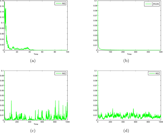
  Trajectories of model (4) with $b=0.4$, $b_{1}=0.2$, $T(t)=0.25+0.1\sin t$, $\xi =0.3$, $\lambda =0.2$, $\rho =0.1$, $\beta _{2}^{2}=0.1$, $\beta _{3}^{2}=0.2$. (a) $\beta _{1}^{2}=0.36$, which reflects the extermination of the species. (b) $\beta _{1}^{2}=0.3$, which reflects the nonpersistence in mean of the species. (c) $\beta _{1}^{2}=0.25$, which reflects the weak persistence of the species. (d) $\beta _{1}^{2}=0.04$, which reflects the permanence of the species

• 2. In Fig. 1(b), $\beta _{1}^{2}=0.3$, and hence $\Lambda =0$. Then from Theorem 3 we deduce that $\lim_{t\rightarrow +\infty }t^{-1}\int _{0}^{t} \Phi (s) \,\mathrm{d}s=0$. See Fig. 1(b).

• 3. In Fig. 1(c), $\beta _{1}^{2}=0.25$, and hence $\Lambda =0.025$. Then from Theorem 4 we deduce that $\limsup_{t\rightarrow +\infty }\Phi (t)>0$. See Fig. 1(c).

• 4. In Fig. 1(d), $\beta _{1}^{2}=0.04$, and hence

  $$ \overline{\Lambda }=b-\frac{1}{2} \beta _{1}^{2}- \limsup_{t \rightarrow +\infty }H_{1}\bigl(T(t)\bigr)=0.03. $$

  Then from Theorem 5 we deduce that $\Phi (t)$ is permanent. See Fig. 1(d).

To finish this paper, we want to point out that our model (7) may be used to describe the effect of pollution in the usual situation, but it may not well describe some extreme pollution cases (for instance, some extreme examples given in Sect. 1). For these extreme cases, more complicate models should be constructed. We leave these problems for further research.