
Depth Contours and Coastline Generalization for Harbour and Approach Nautical Charts


1
Cartography Laboratory, School of Rural and Surveying Engineering, National Technical University of Athens, 15780 Zografou, Greece
2
National Ocean Service NOAA Office of Coast Survey, Silver Spring, MD 20910, USA
*
Author to whom correspondence should be addressed.
ISPRS Int. J. Geo-Inf. 2021, 10(4), 197; https://doi.org/10.3390/ijgi10040197
Submission received: 16 January 2021
/
Revised: 8 March 2021
/
Accepted: 22 March 2021
/
Published: 25 March 2021
Abstract
:Generalization of nautical charts and electronic nautical charts (ENCs) is a critical process which aims at the safety of navigation and clear cartographic presentation. This paper elaborates on the problem of depth contours and coastline generalization—natural and artificial—for medium-scale charts (harbour and approach) taking into account International Hydrographic Organization (IHO) standards, hydrographic offices’ (HOs) best practices and cartographic literature. Additional factors considered are scale, depth, and seafloor characteristics. The proposed method for depth contour generalization utilizes contours created from high-resolution digital elevation models (DEMs) or those already portrayed on nautical charts. Moreover, it ensures consistency with generalized soundings. Regarding natural coastline generalization, the focus was on managing the resolution, while maintaining the shape, and on the islands. For the provision of a suitable generalization solution for the artificial shoreline, it was preprocessed in order to automatically recognize the shape of each structure as perceived by humans (e.g., a pier that looks like a T). The proposed generalization methodology is implemented with custom-developed routines utilizing standard geo-processing functions available in a geographic information system (GIS) environment and thus can be adopted by hydrographic agencies to support their ENC and nautical chart production. The methodology has been tested in the New York Lower Bay area in the U.S.A. Results have successfully delineated depth contours and coastline at scales 1:10 K, 1:20 K, 1:40 K and 1:80 K.
1. Introduction
The cartographic rules are different for depth areas and contours in paper charts and their digital form (raster navigational chart) compared to electronic nautical charts (ENCs). In ENCs, it is important to define depth areas (i.e., contiguous depth contours bounding the depth areas), whereas in paper charts there is no need to define depth areas and broken sections of contour lines can be used for the chart. Data to derive water depths are collected using tidally-referenced surveys, also known as hydrographic surveys, that measure the bottom and detect objects that are dangerous for navigation (e.g., rocks and wrecks). Common survey technologies to map the seafloor are acoustic technologies (such as multibeam echosounders, MBES) and optical technologies (such as, airborne lidar bathymetry, ALB). Using rounding rules, cartographers extract contours (and soundings) for portrayals on nautical charts from these data sources. Although one would expect a fully automated process to be already available, depth contours and soundings portrayal is still a (semi-)manual process [1]. The two main reasons are the data volume and the resulting shape of the depth contours that need to contain all soundings within a value range of the two bounding contours. It is quite a challenge to address these two issues, while trying to maintain the contour line portrayal on a number of scales. In addition to bathymetry, high-resolution accurate coastline data are collected from detailed light detection and ranging (lidar) survey measurements, high-resolution tidally-referenced imagery and topographic surveys. Similar to depth contours, the coastline needs to be generalized according to chart scale [2]. The use of the coastline is not limited only for nautical charts. A frequently updated shoreline supports various applications including coastal and marine spatial planning, tsunami and storm surge modeling, hazard delineation and mitigation, environmental studies, and assists in updated nautical chart production [3].
This paper addresses depth contours and coastline generalization based on published International Hydrographic Organization (IHO) standards and cartographic practices adopted by hydrographic organizations (HOs). The proposed methods deal with the generalization problem in the following framework:
- A high-resolution digital elevation model (DEM, 5 m) vertically referenced to the chart datum as a source for depth contours.
- High-resolution measurements for the coastline.
- The scales of the target nautical charts are 1:10 K, 1:20 K, 1:40 K and 1:80 K (harbour and approach scale ranges).
- The generalization procedures developed in this study should be standard geoprocessing functions available in a geographic information system (GIS) environment in order to allow easy implementation and support chart production, thus reducing production time and costs.
- Soundings, which are the most critical features in nautical charting and have a strict topological relationship with both shoreline and depth contours, are also generalized to show the configuration of the seafloor for safe navigation [7]. The generalized soundings are used as a critical element in the contours generalization procedure as it will be documented in this paper.
The paper is organized as follows: Section 2 provides background material on depth contours and coastline generalization; Section 3 and Section 4 elaborate on the proposed methodology for depth contours and coastline generalization; Section 5 describes the case study and Section 6 discusses the results and presents plans for future research. Appendix A is a detailed guide for the generalization steps followed. Appendix B provides key artificial coastline features, generalization practices, measures and procedures utilized for shape identification and generalization. Appendix C describes the proposed contours generalization procedure utilizing ArcGIS geoprocessing tools along with the values of the parameters involved.
2. Background
The purpose of depth contours and elevation points in a nautical chart are different than those of a topographic map. The depth values in a chart are rounded to less depth for safety of navigation. For similar reasons, depth content in nautical charts provides a more schematic representation of the seafloor morphology. Starting from the seafloor modeled by a set of soundings and contours extracted from the bathymetric database, the cartographer would work in practice by selecting spot soundings and contours according to the relevance of the submarine features they model [8]. Thus, distinct generalization approaches in terms of constraints, rules, operators etc. are applied. In the following paragraphs, standards, constraints and existing practices for depth contours and coastline generalization are reviewed.
2.1. Depth Contours Standards and Constraints
The study uses a number of guidelines for contours generalization that are made available through the IHO standards, namely IHO S-4, IHO S-57, and IHO S-58 [5,6,7]. Constraints result from the need for safe navigation and clear presentation. The generalization requirements can be organized according to different classes of constraint [9]. Referring to Ruas and Plazanet’s classification [10], constraints in depth contour generalization for nautical charts can be categorized as follows:
- The legibility constraint: generalized contours must be legible by observing a minimum size or distance between them;
- The position and shape constraints: absolute position and shape of contours must be maintained as much as possible;
- The structural and topological constraints: spatial relationships between contours and soundings are maintained;
- The functional constraint specific to the purpose of the map: on a nautical chart, functional constraints are the safety constraint indicating that a reported depth cannot be greater than the real depth and the preservation of navigation routes.
Nautical chart generalization proceeds with the inclusion of shoals lying seaward of the principal contour [4]. Contours should be smoothed (i.e., reduce sharp angles in polylines or polygons in order to improve aesthetic or cartographic quality) only where it is necessary and eliminate confusion to mariners. For example, the removal of intricacies, which would confuse mariners and the smoothing of the severely indented contours and pushing the contours seaward to include deeper water depths within shallower contours [4]. In addition, generalized depth contours must not cross areas shallower than the depth area (e.g., values shallower than depth range value i.e., “DRVAL 1” Feature Object Attribute in S-57). Depth contours can be omitted in very steep slopes, if space permits the deepest and the shallowest contours should be retained. More specific constraints for depth contour generalization cover special cases e.g., channels [11]. Depth contours as linear features must not be encoded with a vertex density greater than 0.3 mm at compilation scale [6]. This restriction is further elaborated by United States’ National Oceanic and Atmospheric Administration (NOAA) and a threshold of 0.4 mm is proposed [12].
An important aspect is the relation between contours and soundings. Soundings and contours must be used to complement each other in giving a reasonable representation of the seafloor, including all significant breaks of slope. Depth contours must be drawn in such a way that no sounding having exactly the same value as the contour line will appear on the deep-water side of the contour, except where the soundings represent isolated shoals [4,6]. In this case, they must be encircled by a depth contour of the same value or by a danger line. Depth contours shall not “touch” the sounding figures and shall be drawn around them [11].
2.2. Depth Contours Generalization-Related Work
In cartographic literature, two main approaches can be used as guidelines for contour generalization [1]. In the first approach, the seafloor surface is generalized and depth contours are extracted from the simplified surface. This approach pertains to model generalization as it is robust, fast and allows depth contours to be generated at various scales. In the second approach, contours from a larger scale chart or extracted from a DEM are directly generalized. In this study, the second approach is followed because it is more reliable, thus contributing to the safety of navigation. Furthermore, it results in clear presentation and aesthetics with respect to the input contours and the aforementioned constraints that provide the mariner with a concise understanding of the sea bottom.
In the framework of the second approach, an important issue for depth contour generalization is the selection of the appropriate generalization operators. By examining the way nautical cartographers manually perform depth contour generalization from a large scale to a small scale chart, it is observed that contours are simplified and smoothed [13]. Changes to the shape of polyline (open contours) and polygon contours (closed contours) can only result in moving the curves seaward compared to the original location of the curve [11]. Based on a minimum threshold distance, polygon contours are aggregated with each other. Eventually the polygon contours are aggregated with the polyline contour in the vicinity. Comparison of contours extracted directly from the DEM and those displayed on a hydrographic chart from the Royal Australian Navy [1] showed that pits contained in the DEM are removed from the chart, while peaks are either preserved in the chart or integrated with another contour, and groups of nearby contours are aggregated [1]. In [14], the seafloor is described using a feature tree that provides a hierarchical structure built from a depth contour graph. Generalization operators such as smoothing, displacement, deletion, aggregation and enlargement are applied to depth contours to improve map legibility and aesthetics [15]. Based on this idea, Zhang and Guilbert [16] introduced a multi-agent system (MAS) for depth contours generalization, which was implemented and tested on a set of contours at 1:50,000 scale provided by the French Hydrographic and Oceanographic Service (Service Hydrographique et Océanographique de la Marine, SHOM) [15]. The results satisfy the legibility constraint, however the morphology of the seafloor seems to be over-smoothed due to regular distances between depth contours. The need of extending the definition of features to deal with segmented contours and adding a segment removal operator is necessary.
Regarding depth contour smoothing, two methods observe the shoal-bias constraint [2]: double buffering and spline-snake. Double-buffering is a common GIS function, commonly employed in commercial hydrographic software, where a new line is created within a specified distance from the nearest point on the original line (or polygon) [1]. If the new line is then buffered back in the opposite direction, a generalized version of the original line is created. It effectively takes into account the safety constraint as well as performs a form of aggregation [1]. It is important to note that the generalized line honors the seaward extent of the contour [17]. In the second method, the spline-snake model, a spline which is a piecewise polynomial function that is by definition smooth is used. Guilbert and Lin [18] and Guilbert and Saux [19] use splines in combination with a snake model to perform smoothing and displacement. Their method observes the safety constraint and results in smooth contours at the same time. Moreover, Miao and Calder [20] proposed an improved method of using B-splines for gradual contour generalization for nautical charts.
From the review of the aforementioned depth contour generalization methods, it was revealed that the seafloor description is a critical factor that guides depth contour generalization. Additionally, information was collected on the operators that can be applied and the available smoothing algorithms that observe the shoal-bias constraint. However, the proposed methodologies [14,15,16] require specific data encoding structures and tools that do not exist in a standard GIS. As a result, it is difficult to apply them in a nautical chart production environment because they lack compatibility with IHO encoding standards [4,5,6] that use Open Geospatial Consortium (OGC) Simple features enhanced with specific attributes. Moreover, existing methodologies address depth contours that are portrayed on nautical charts [15], whereas currently the trend is to generalize raw contours extracted from high-resolution DEMs. In conjunction with the conclusions extracted from the review of papers on soundings generalization [7], it was revealed that soundings and depth contours generalization are not addressed within the same framework in order to ensure consistency. Regarding commercial-off-the-shelf (COTS) tools that are utilized for nautical chart production, to authors’ knowledge, there is no solution that efficiently solves the nautical chart generalization problem of the above features. This research approach adopts seafloor description as an important factor that guides depth contours generalization. At the same time, it proposes a generalization method that can handle depth contours already portrayed on nautical charts but also those extracted from DEMs, integrates them with generalized soundings and can be implemented in a standard GIS environment.
2.3. Coastline Standards and Constraints Implementation
General guidelines for coastline generalization [4] refer to two main requirements: safe navigation and clear presentation. Safe navigation is ensured if the coastline is displaced only seawards and clear presentation when the line symbol does not self-intersect/self-overlap or overlaps/intersects with neighbor features. In addition to this, the cartographer is encouraged to “eliminate the least essential information” by the application of simplification and smoothing. The coastline axis displacement limit [11] should be also taken into consideration. More specifically, one-half the symbol line weight plus a +/−0.15 millimeter maximum displacement is acceptable. Based on ENC validation checks [6], the coastline as a line feature must not be encoded at a point density higher than 0.3 mm at compilation scale. This restriction is further elaborated by NOAA and an upper limit of 0.4 mm is proposed [12]. Consequently, the deletion of vertices based on the vertex distance criteria is strongly recommended. In bays and embayments, vertex points that push the shoreline ashore (within a 0.3 mm/scale tolerance) should be selected.
Islands and islets are considered more complex for cartographic judgment and require special handling. If the width and the length of the islands are both greater than 0.8 mm/scale (i.e., the width and length are both greater than 8 m for 1:10 K, 16 m for 1:20 K, 32 m for 1:40 K and 64 m for 1:80 K), the islands are maintained and a land area is created [21]. If the width and the length of an islet are both less than 0.8 mm/scale, the islet collapses to a point feature. Finally, if the width and the length of an islet are greater than 0.8 mm/scale along one direction but less than 0.8 mm/scale along the other, the elongated islet collapses to a single line. In cases that the detached features are close to the shoreline (e.g., land areas or points that are less than 8 m for 1:10 K, 16 m for 1:20 K, 32 m for 1:40 K and 64 m for 1:80 K to the shoreline), the detached features are merged to the shoreline (i.e., the modified shoreline should be on the outer boundary of the features).
Regarding man-made coastline (i.e., IHO S-57 ShoreLine CONStruction object, SLCONS [5]), specific details for the management of piers or other structures are based on their shape, geometric characteristics, such as size, width and relative position to the coastline [21]. When the width of a pier or a structure is less than 0.4 mm, then only one side of the man-made feature is selected. Piers or other structures that are smaller than 0.8 mm or are less than 0.8 mm from the shoreline are deleted.
2.4. Coastline Generalization-Related Work
Coastline generalization is considered a popular research topic in cartography. A number of line simplification algorithms appear in literature and are applied in coastline simplification such as geometric measures methods [22], topological objective methods [23], natural principle method [24], the shape-preserving method [25], etc. In this research, the focus is set on compliance with the IHO standards. As a result, natural coastline vertex density that is of high importance for ENCs is given priority. Regarding artificial coastline generalization, a major issue towards automation is the need to describe the shape of each structure as perceived by humans (e.g., a pier that looks like a T) in order to apply the appropriate generalization solution/algorithm. This paper proposes a new method that automatically recognizes the shape of key artificial coastline structures through preprocessing and thus supports the automation of the generalization process.
3. Depth Contours Generalization across Scales
The analysis of rules, constraints and proposed procedures for depth contour generalization lead to the design and development of a comprehensive generalization framework that is discussed in the following paragraphs.
3.1. Depth Contours Generalization Framework
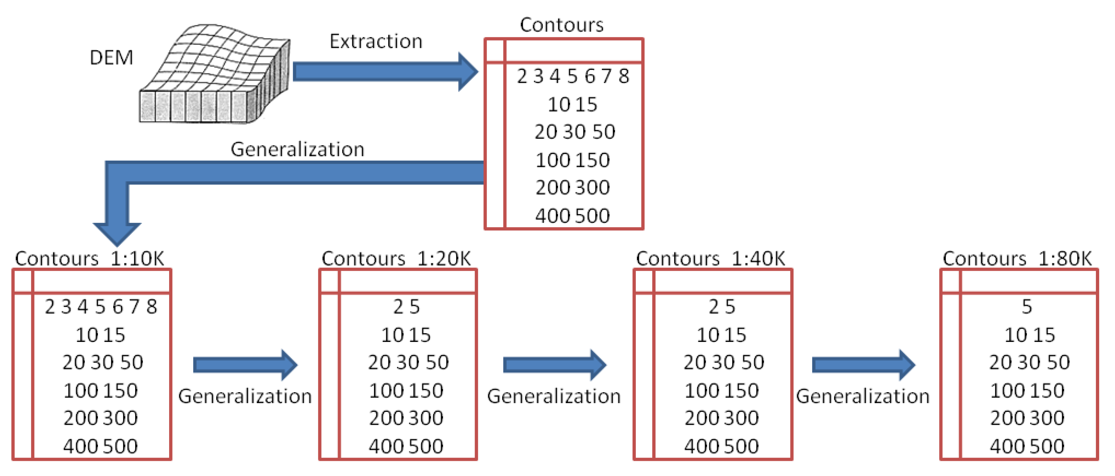
Metric depth curves portrayed on ENCs are set in relation to the compilation scale. This study addresses scales for harbour and approach nautical charts. Τhe standard set of integer meter depth values for new gridded ENC depth contours [12] are based on depth intervals specified in the IHO S-101 Product Specification [26]. A group of contours (e.g., 2, 3, 4, 5, 6, 7, 8, 10, 15, 20, 30, 50, 100, 150, 200, 300, 400, and 500 m) is recommended for portrayal at the largest scale (in this case, 1:10 K) and a subset from this initial group is portrayed at smaller scales (see Figure 1). Τhe selection of a subgroup of the contours portrayed at the larger scale for portrayal at the smaller scale is compliant with the “ladder approach” (Figure 1). This implies that depth contours portrayed at a smaller scale will be the result of the generalization of those portrayed at the larger scale. Thus contour consistency across scales is ensured. Moreover, depth areas are created following the completion of depth contour generalization.
This approach is also in accordance with the adoption of the “ladder approach” for soundings generalization [7]. The need to portray a subset of the extremely dense original soundings from the DEM on charts across scales downgrades DEM generalization as a solution. Thus, any sounding portrayed at a smaller scale chart is also depicted at the larger scale as required by IHO specifications. Eventually the “ladder approach” is satisfied by both depth contours and soundings resulting from generalization.
3.2. Depth Contours Generalization Methodology
Nowadays, high-accuracy seafloor measurement methods lead to the creation of high-resolution DEMs. As a result, it is a common practice to extract depth contours directly from the DEM by intersecting at certain depth values. The extracted depth contours are usually subject to generalization. Depth contours generalization refers to the following two cases:
- Those extracted from the DEM need to be generalized for portrayal at the largest scale of the nautical charts series e.g., 1:10 K. Depending on the gridding interpolation method, these contours can seem “jagged”, especially as the morphology of the seafloor changes abruptly. They contain many “island” contours due to local minima and maxima. These artifacts are the result of measurement noise that is present in the MBES or ALB datasets; that is, the variation in depth between two close samples can be different than in reality. The artifact can be observed even after the dataset has been statistically cleaned [1,27].
- Those portrayed at the larger scale of the nautical charts series need to be generalized for portrayal at smaller scales (e.g., 1:20 K for NOAA) according to the ladder approach. In the same way, the 1:20 K scale contours are generalized for portrayal at 1:40 K scale and others.
In this research, both generalization cases are confronted and a common generalization restriction is applied: each depth contour line should be generalized individually. Generalization starts with the processing of the shallow contours and continues with the deep ones. This is in accordance to the general principle of ensuring safe navigation in order to guarantee displacement of the generalized depth contours seaward to the deep-sea areas [11]. Therefore, each contour will depend on the already generalized shallower ones.
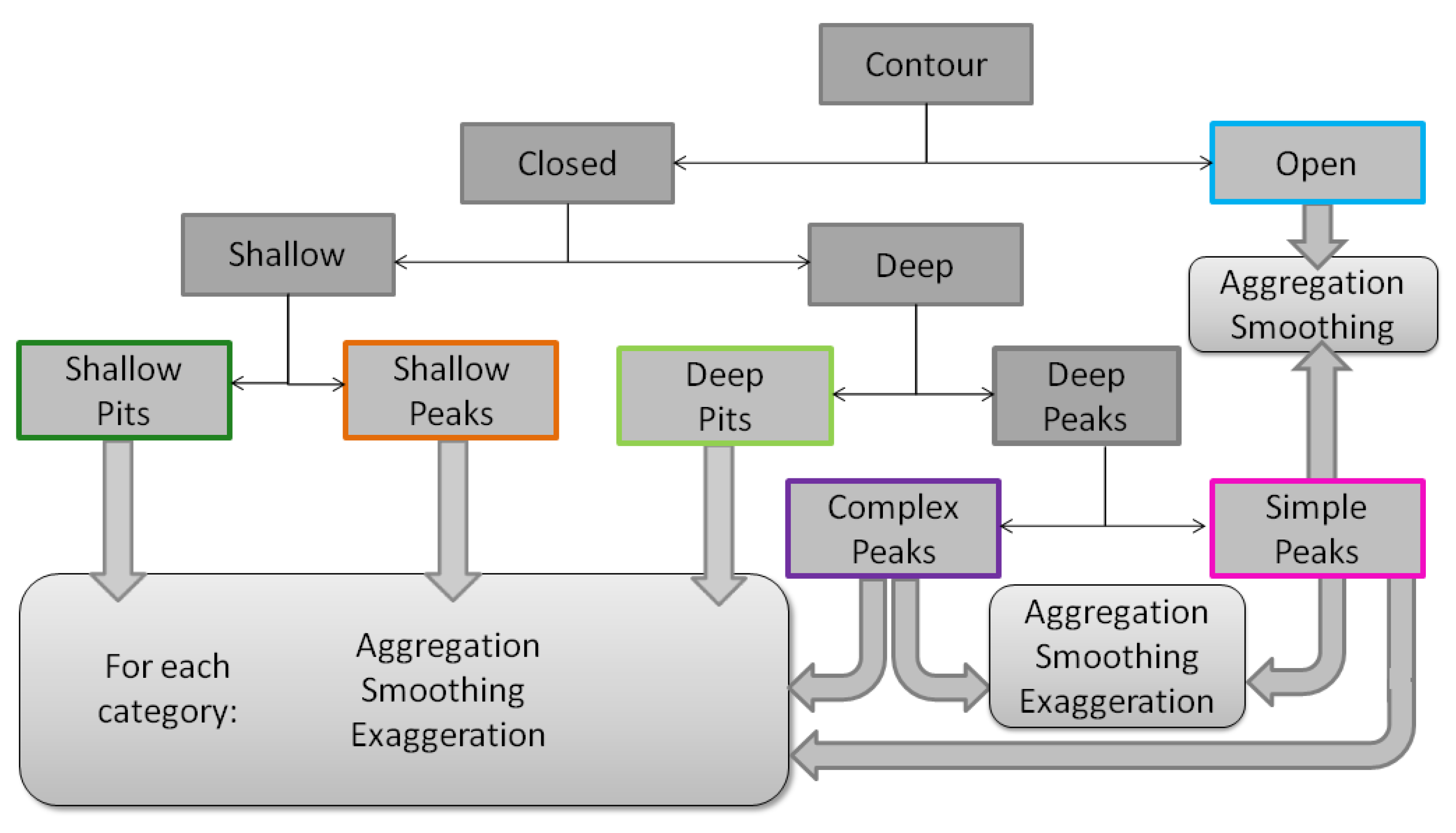
In order to perform generalization that maintains the morphology characteristics of the seabed, it is important to identify its structure utilizing characteristic properties of the contours [14,15]. In contrast to existing methods [14,15], in this study each contour is initially pre-processed and enriched with auxiliary information contributing to seafloor description and generalization. For each contour, a number of properties are assessed that include: geometry (e.g., open/closed), relative position to the open contour (e.g., shallow area/deep area), the depths located within them (e.g., peaks /pits) and topological relations between closed contours (e.g., no contain/no within, contain other, within other). Contour lines are classified based on these properties (Figure 2 and Figure 3). All contour lines are divided into Open polylines and Closed polylines that are converted into polygons. Moreover, Closed contours are classified into Shallow area contours and Deep area contours with respect to the open contour under examination. The Open contour is, therefore, considered as a barrier that influences the processing of the closed contours. Each Closed (polygon) contour is characterized as a pit or a peak in relation to the contour value and the depths located within. Finally, the topological relations between all Closed contours in the area are identified and classified in one of the following three categories: (a) contours that do not contain or are not contained in other contours, (b) contours that contain other contours, and (c) contours contained in other contours. Deep peaks that do not contain or are not contained in other contours are defined as Simple Peaks and the other two categories are considered as Complex Peaks.
Based on the classification definitions mentioned above, depth contours generalization proceeds using the decision tree in Figure 2:
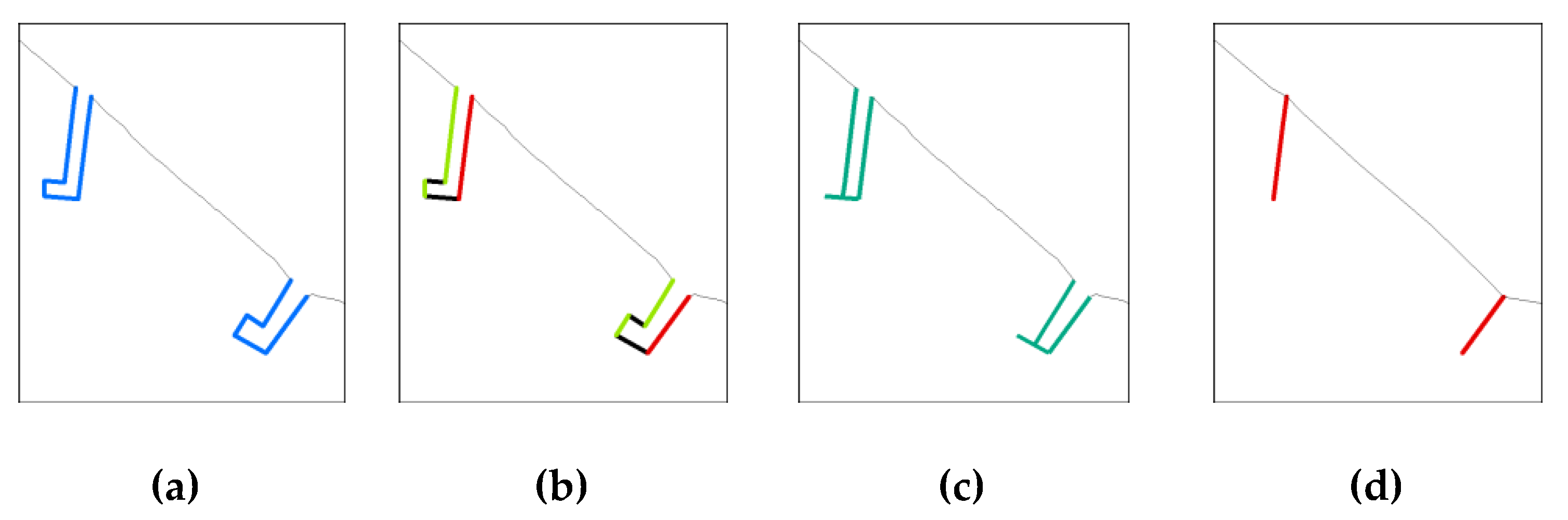
- Simple Peaks located in proximity to Open contour: Some of the Simple Peaks are very close to the Open contour in relation to the chart scale and thus should be aggregated with this contour, moving the Open contour to the deeper area. Only Simple peaks can be aggregated with the Open contour (Figure 3a,b). Aggregation (Figure 4 and Figure 5) and smoothing operators are applied with the double buffering method.
- Simple Peaks located in proximity to Complex Peaks: Simple peaks that are not located close to the Open contours in relation to the chart scale are checked for their proximity with the Complex Peaks (Figure 3a,c). Thus, these Simple Peaks are aggregated with the Complex Peaks (Figure 4 and Figure 5).
- Simple Peaks not in proximity to Open contour or Complex Peaks: Simple peaks that are not located close to the Open contours or Complex Peaks are aggregated if they are in proximity to each other.
- Deep Pits or Shallow pits: Pits located in the shallow or deep area that include soundings are evaluated and aggregated if they are in proximity to each other (Figure 3a,d,e). It is recommended to omit Pits that do not include soundings.
- Shallow Peaks: Shallow Peaks are evaluated and aggregated if they are in proximity to each other (Figure 3a,e).
- Exaggeration of Peaks or Pits that include a sounding: Peaks or Pits that include a sounding should be checked against the minimum area requirement for sounding portrayal. This evaluation ensures that the area available for the depiction of the sounding is adequate. If the area available is not adequate, closed contours need to be expanded using the exaggeration operator (Figure 3 and Figure 4).
Depth contours resulting from aggregation should not cross any other chart feature. This is especially true for group 1 bounding line features that are charted boundaries for “skin of the Earth” area features, such as coastline, dredged areas, and unsurveyed areas [5,6]. Consequently, these group 1 bounding line features and other depth contours in the vicinity are used as barriers during aggregation process. At smaller chart scales, the distance/space required between objects to be portrayed separately becomes larger. Therefore, larger distances are used in aggregation and exaggeration (Figure 3). Additional simplification and/or smoothing can be applied to the resulting contours if needed depending on line granularity.
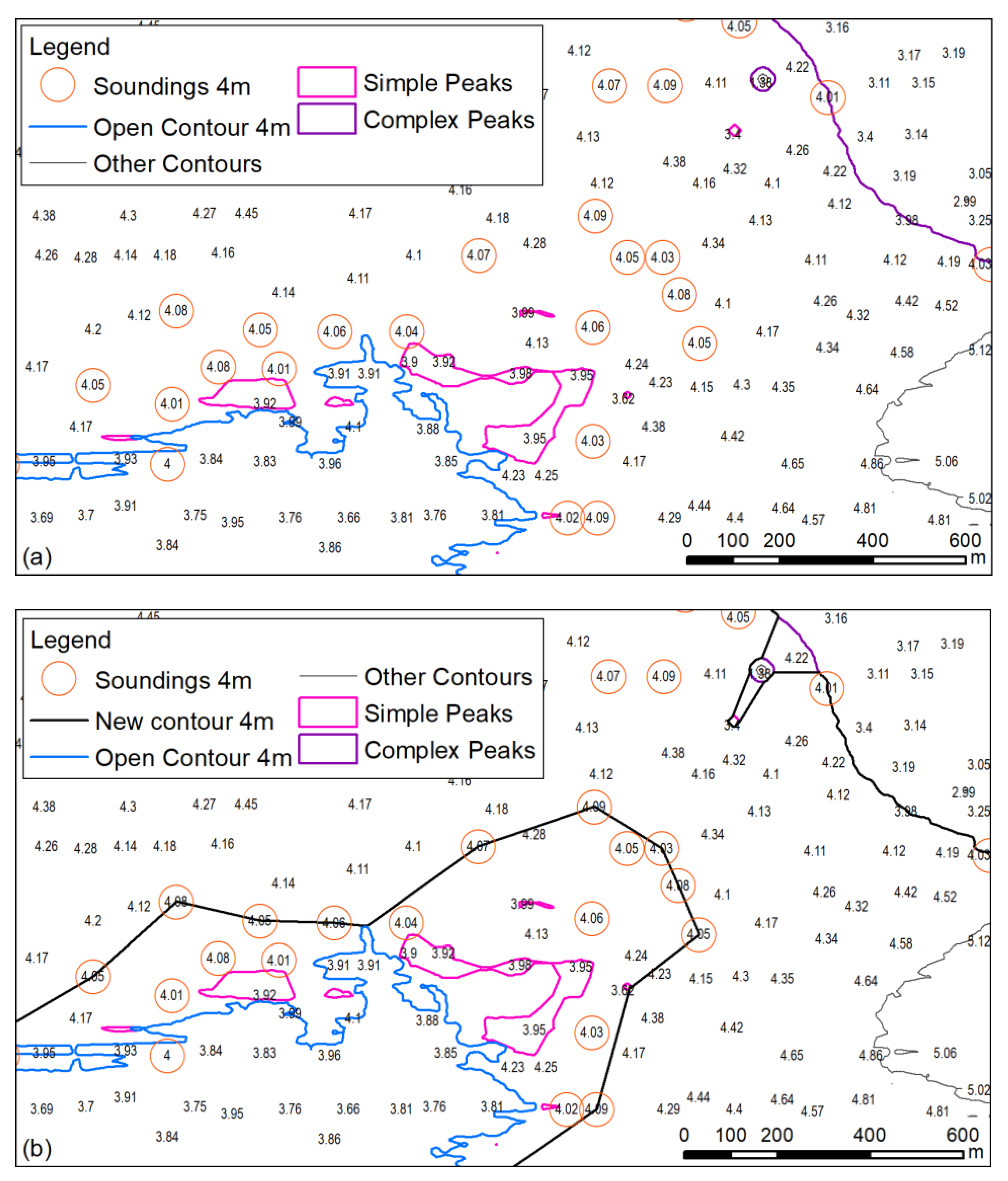
One of the main qualities of a nautical chart is the logical consistency between features portrayed on the chart. Depth contours and soundings originate from the same data source. However, an incompatibility may be observed in cases where a contour does not contain all the soundings with depths equal to its value within its depth range (Figure 5a). This issue is a result of the soundings rounding, and not due to an error in the contours which are extracted from the DEM and appropriately generalized. For example in Figure 5a, a number of soundings with depth value greater than 4 m e.g., 4.04, 4.06, 4.07 etc., are rounded to 4 m according to the rounding specifications [4]. Thus, these soundings appear as missed by the generalized 4 m depth contour. In order to ensure consistency, the 4 m depth contour should be shifted and forced to pass through all 4 m soundings. Consequently, the proposed procedure in this study is to shift the contours towards the deeper side in order to pass through soundings with depth equal to the depth value of the contours that are portrayed on the chart (Figure 5b). This procedure is applied to both open and closed contours only during the generalization of the raw contours for the larger scale i.e., 1:10 K. For the smaller scales, as the soundings are subgroups of the ones portrayed at the larger scale due to “ladder generalization” [7], there are no inconsistency issues between the contours and the soundings.
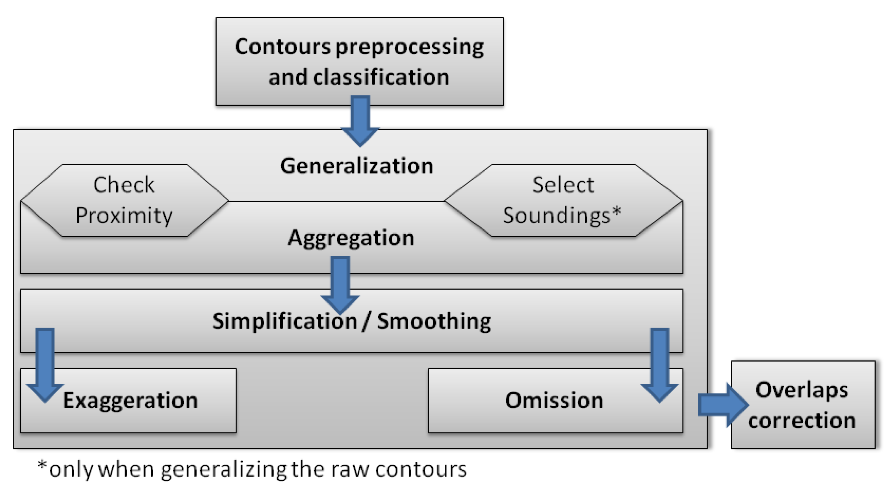
In conclusion, the sequence of operations for contour generalization is the following (Figure 6):
- Contours preprocessing and classification: Identify seabed structure and classify depth contours as explained (see Figure 2).
- Generalization:
- Check proximity between contours to find those that will be aggregated e.g., assess Simple Peaks close to Open depth contour, Simple Peaks close to Complex Peaks etc.
- Select soundings: when generalizing the raw contours for the larger scale i.e., 1:10K locate portrayed soundings with depth equal to the contour value under examination and located close to it.
- Aggregation is applied for the following cases: a. Open Contours, Simple Peaks, b. Complex Peaks, Simple Peaks, c. Simple Peaks, d. Deep Pits, e. Shallow Peaks, f. Shallow Pits. When generalizing the raw contours for the larger scale i.e., 1:10 K soundings are taken into account in the aggregation process.
- Simplify and/or smooth contours resulting from aggregation.
- Exaggerate small closed contours that include a sounding.
- Overlaps correction: delete contours that overlap with dredged areas or the coastline.
4. Coastline Generalization
The natural and artificial coastlines are processed separately, in accordance with the analysis of the guidelines and the constraints for coastline generalization. Although natural coastline generalization is an open research item, in this study generalization focuses on the resolution and the islands while preserving their inherent characteristics. Artificial coastline is composed of a number of structures e.g., piers. These structures and their shapes should be identified and characterized for successful generalization.
4.1. Natural Coastline
Natural coastline is generalized through a simplification process in order to reach the expected vertices density (resolution) foreseen by the specifications. In this study the minimum threshold is 0.4 mm to the charted scale. Vertices that do not meet this distance requirement should be removed. As a result, the application of any other simplification algorithm is excluded. Vertex elimination based on distance does not impact the original coastline shape due to the high density of the source data.
Before vertex elimination, a preprocessing phase takes place. This is done in order to maintain nautical chart consistency. When a feature is deleted, care must be taken to ensure that this deletion does not affect another one [4]. As a result, natural coastline vertices that are common with artificial coastline structures portrayed at the compilation scale should not be eliminated during simplification. These vertices need to be identified and flagged in order to be preserved. Line segments that have a common vertex with artificial coastline are identified during this preprocessing phase (see Appendix A.1).
Islands and islets are defined as polygonal coastline features. The distance between the islands/islets to the mainland coastline is computed and islands/islets are characterized in terms of their area. Minimum bounding rectangles are created for each island/islet in order to assess properties, such as width and length. Properties assessment, islets characterization, elongated islets or those too close to the coastline ones, are implemented with specific procedures (see Appendix A.2).
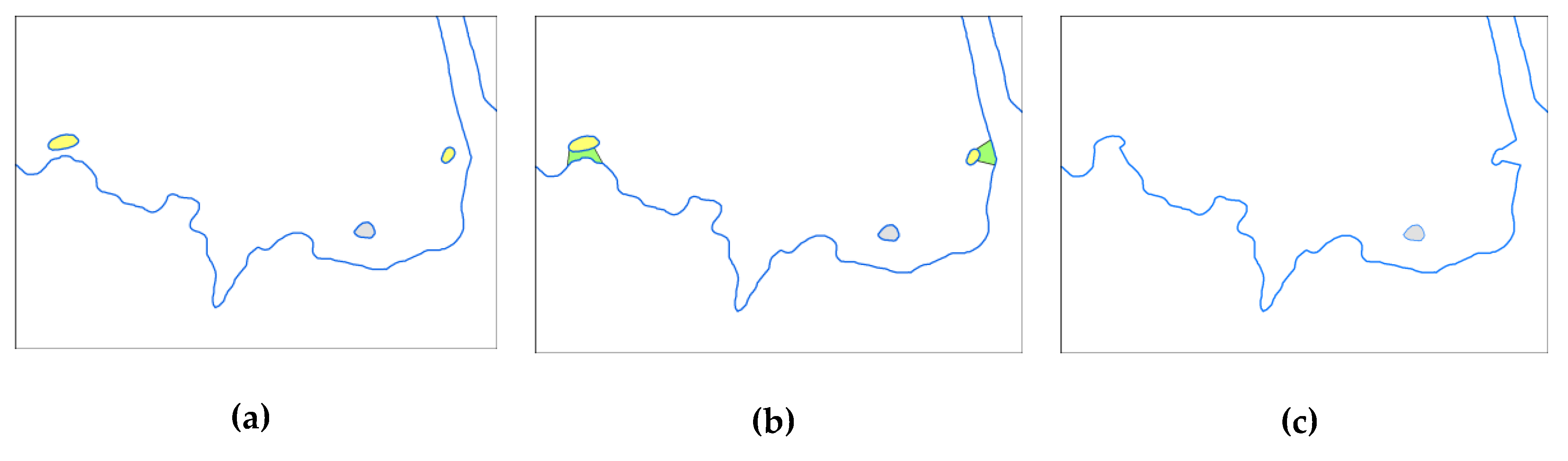
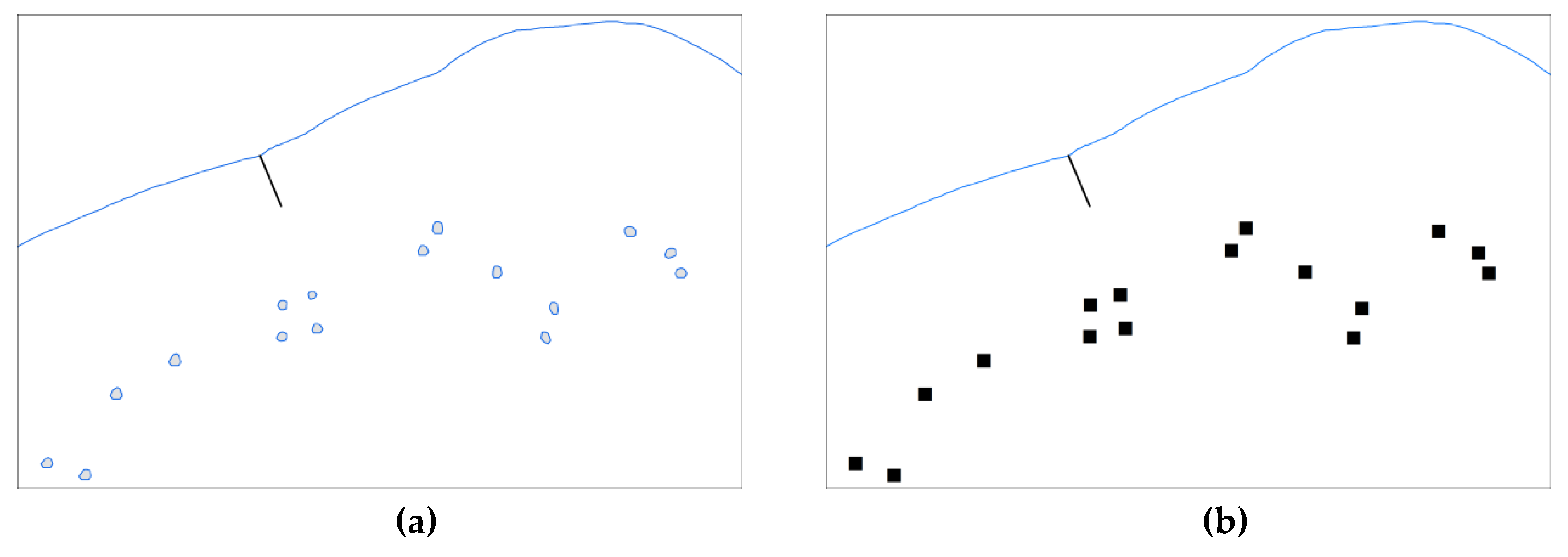
The next step after preprocessing and data enhancement is applying generalization operators, such as aggregation, collapse, and simplification following natural coastline characteristics and the cartographic guidelines. First, specific GIS functions are utilized for generalization of island features (see Appendix A.3) in order to aggregate islands in proximity to the mainland with the shoreline (Figure 7). Very small islets are converted to point features based on their centroid (Figure 8) and small elongated islets are converted to lines (Figure 9) (see constraints in Section 2.3). Examples shown in Figure 7, Figure 8 and Figure 9 are automatically created with the developed GIS functions.
Finally, natural coastline is simplified in order to achieve vertices density according to the guidelines, e.g., max 0.4 mm per scale. Line segments resulting from the natural coastline preprocessing step are processed in sequence (Figure 10). All coastline segments that are not connected to the artificial coastline and are smaller than the tolerance distance are deleted. When a coastline segment is deleted, the next coastline segment is snapped to the previous one. As a result, a new coastline feature is created from the new coastline segments with all the original attributes transferred/updated to the new coastline feature.
4.2. Artificial Coastline
An artificial coastline consists of specific structures such as pier, breakwater etc. addressed in the CATSLC (i.e., IHO S-57 CATegory of ShoreLine Construction) attribute [5]. In order to properly apply generalization, specific characteristics of the structures describing their shape should be identified through preprocessing. Since these structures vary from simple to very complex, it is feasible to recognize and handle in a uniform way only those which are similar to geometric shapes. Special and very complex cases need to be handled individually by the experienced cartographer.
The generalization step for artificial coastlines is carried out in stages. First, all connected segments that form an artificial coastline structure are assessed. Then, each artificial structure is classified based on its specific characteristics regarding shape. For example a T-shape pier is classified using its inherent properties e.g., length, width and other properties identified through preprocessing e.g., distance from the shoreline, azimuth with respect to a given reference etc. For every structure, elements that would be altered due to generalization are identified, e.g., a T-shape structure is analyzed to vertical axis and cup. These elements are not semantically flagged originally since structures are stored as simple line segments. Finally, generalization in accordance with the specifications is applied.
The minimum bounding rectangle (MBR) is the key auxiliary structure that allows for the identification of segments’ subgroups that are connected and form specific structures. It is created as follows: buffers are generated around artificial coastline segments, overlapping buffers are amalgamated to one polygon and finally a minimum bounding rectangle is created for each polygon. The MBR dimensions such as width, length etc. are added as attributes to the data. Segments in each MBR are considered to represent a structure. Apart from the MBR dimensions, a number of geometric and topological measures/characteristics are considered:
- The number of segments (removal of nodes that do not represent crossings and/or split lines at crossings);
- The distance of segments from the coastline;
- The number of segments connected with the coastline;
- The azimuth of segments and the change of azimuth between consecutive segments.
A number of key artificial coastline features are identified (Figure 11). In Appendix B (Table A1), the measures and procedures utilized for their identification are presented in detail.
Two generalization operators are applied for artificial coastline structures: collapse (minimization of feature dimensions), such as transformation of an L shape into line (Figure 12), a Pi shape to line (Figure 13), a boot shape to line (Figure 14), a T shape to line (Figure 15), and omission such as transformation of T shape (no width) (Figure 16) and Antenna shape (Figure 17) (deletion of certain parts—Figure 17c, or feature deletion—Figure 17d). The collapse function can be applied in generalization cases transitioning from a large-scale chart to a medium-scale chart. Then, omission is applied for generalization cases transitioning from medium-scale charts to small-scale charts. In Appendix B (Table A1), (Figure 11a–l), the generalization practices are presented in detail. Both practices are recorded as Stage A (from a large scale to a medium scale) and Stage B (from a medium scale to a small scale). A critical factor for the omission of any artificial structure that is transverse to the coastline is the length of the structure that describes its distance from the coastline. When this distance is too short in relation to the chart scale, the user is unable to distinguish the structure from the coastline. The use of the collapse operator can lead in many cases to a realistic solution. Obviously, the list of cases identified in this study is neither exclusive nor complete but it aims to provide solutions for the most common ones. It is not possible to develop an automated generalization solution for complex structures with great variability because of the challenge to provide their analytical description. Instead, only the distance from the shoreline can be applied as omission criterion.
In conclusion, the sequence of generalization operations applied to coastline features are as follows:
- Identify structures in artificial coastline and classify them based on their shape to key artificial coastline features (Figure 11). This is done automatically based on the above described procedure.
- Apply the appropriate generalization procedure to each artificial coastline structure based on classification and identified properties (e.g., minimum width and minimum length) and tolerances according to nautical chart compilation scale guidelines (Figure 12, Figure 13, Figure 14, Figure 15, Figure 16 and Figure 17).
- Identify vertices along natural coastline that are common with artificial coastline structures that will be portrayed at the compilation scale (Figure 10).
- Simplify natural coastline by removing vertices too close to each other in order to achieve the distance between vertices according to the specifications (taking into account vertices common with artificial coastline that should not be omitted) (Figure 10).
5. Case Study—Results
5.1. Study Area and Source Data
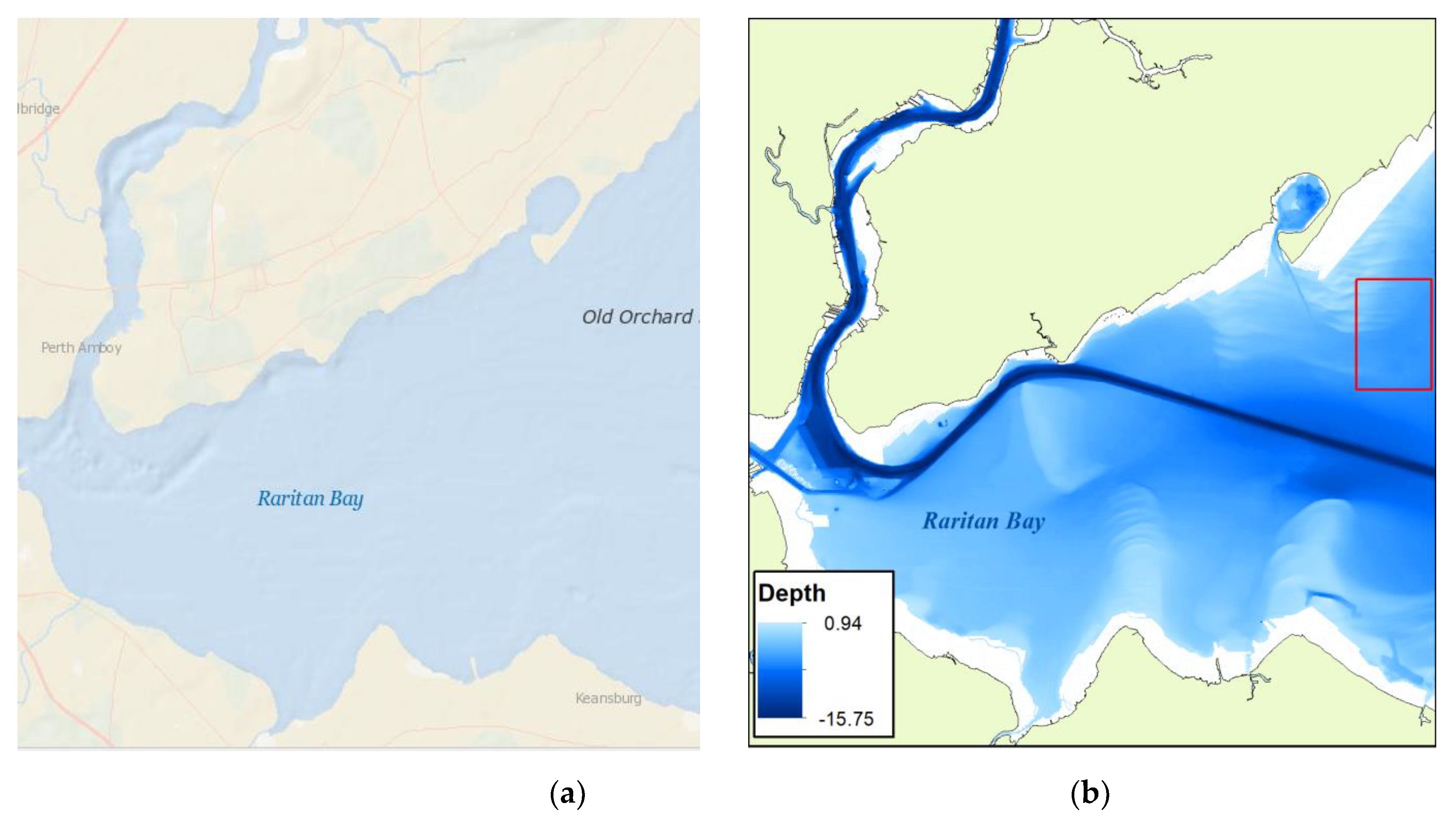
The study area for the aforementioned generalization procedure is the Raritan Bay area. Raritan Bay (Figure 18a) is a bay located at the southern portion of Lower New York Bay between the states of New York and New Jersey and is part of the New York Bight [28]. Bathymetric data of the bottom were generated from NOAA’s National Bathymetry Source [29] at a 5 m resolution DEM over a 110 km2 area (Figure 18b). The depth range of the bathymetry dataset is between 0.94 m above mean lower low water (MLLW) to 15.75 m below MLLW.
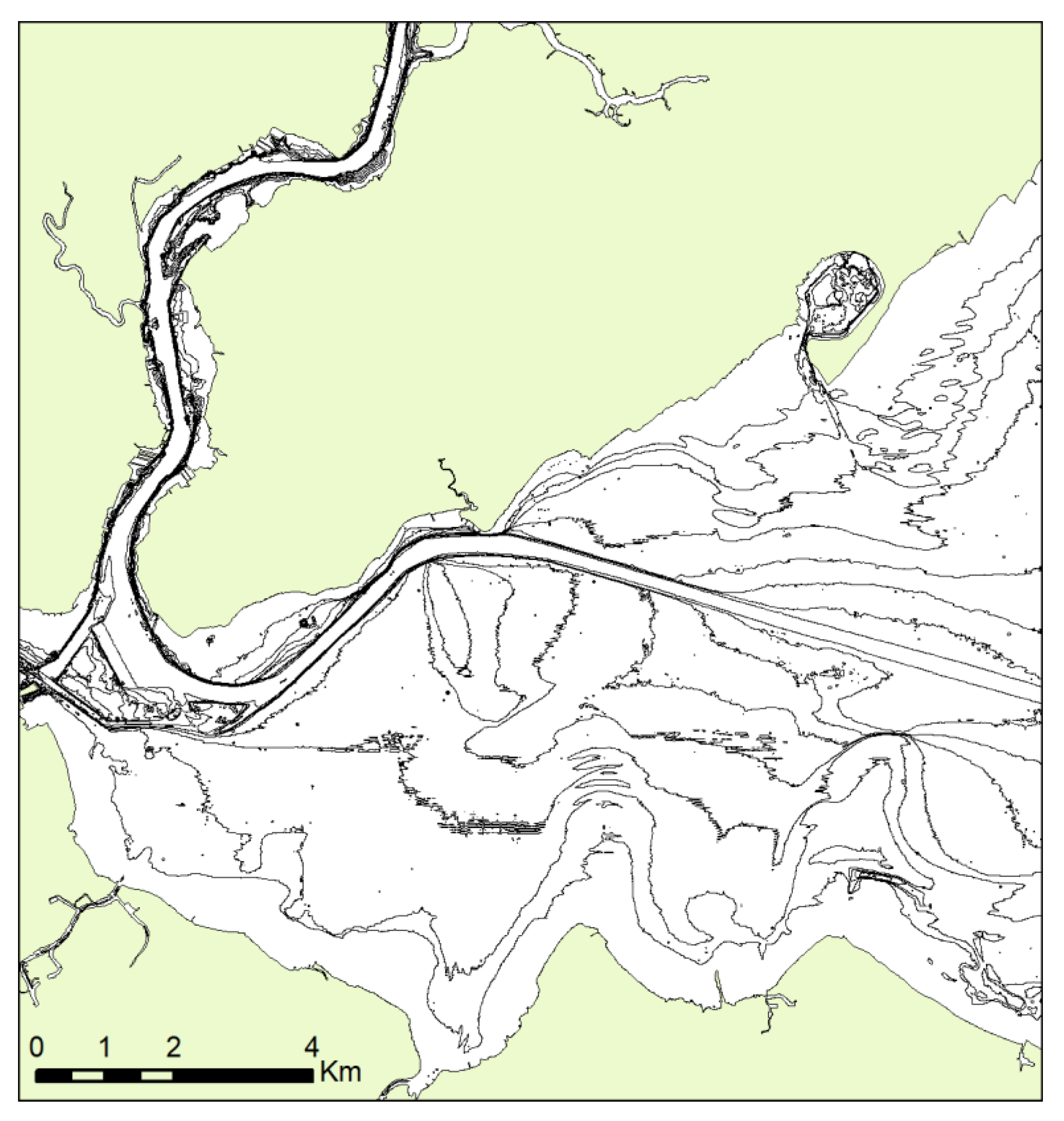
The DEM has gaps and does not cover the area up to the coastline. For the extraction of the contour lines a full coverage DEM for the study area is required in order to avoid fragmented contours. According to key cartographic rules non-surveyed areas will be generated based on the gridded bathymetry. A triangular irregular network (TIN) is created utilizing the coastline and the points resulting from the transformation of the DEM to a point dataset. The resulting TIN is gridded to a new DEM in order to interpolate and fill gaps over non-surveyed areas up to the coastline. Areas with survey data remain intact using the elevation values from the original DEM. Depth contours for scale 1:10K are extracted from the new “complete” DEM. The extracted contours are defined as raw contours that need to be generalized before portrayal on the chart (Figure 19).
NOAA coastline data at scale 1:15 K was used as a reference dataset for testing the generalization procedures for 1:20 K chart products. The 1:20 K dataset is then generalized to obtain the 1:40 K one and the 1:80 K, according to the ladder approach.
5.2. Implementation
The proposed depth contour generalization methodology is implemented using ESRI’s ArcGIS 10.5.1 geo-processing tools in customized routines that apply the set of rules developed and automate the process using geo-processing models. The sequence of the applied procedures and the values of the parameters utilized appear in Appendix C. Distance values for aggregation are larger when generalizing the raw contours portrayal at the larger scale in order to encompass the selected soundings. For contour aggregation, 3 mm at the scale of the chart is used. This is also the minimum size for the closed contours that include a sounding. As scale gets smaller the need for line smoothing diminishes. Smoothing is mostly applied when generalizing raw contours that are more jagged.
The generalization of the coastline is implemented in ArcGIS 10.5.1 as well. A simplification procedure was applied to the raw natural coastline polyline in order to achieve the required vertex density using a Python script. With respect to the artificial coastline generalization, the procedures described previously are as well implemented in ArcGIS utilizing the processing tools available for spatial data along with developed customized routines. All procedures utilize parameters values according to the existing standards.
5.3. Results
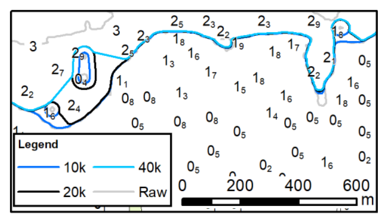
In Figure 20 and Figure 21, one can see examples of the depth contours generalization in extracts of the relevant nautical charts at scales 1:10 K, 1:20 K, 1:40 K and 1:80 K. The portrayed soundings are the results from research published by the authors on soundings generalization [7]. Coastline generalization examples can be found in Figure 22 and Figure 23. Apart from simplification, the first example (Figure 22) includes islands collapsing to points and the second includes aggregation of islands located close to the coastline (Figure 23). Artificial coastline generalization is presented as well. All examples shown in these figures are automatically produced based on developed geo-processing routines.
The resulting compiled nautical charts are reliable, efficient and in accordance with the specifications. Visual evaluation of the resulting nautical charts shows that they provide a clear presentation of the seafloor and there are no inconsistencies between the soundings and the depth contours. The results of the natural coastline simplification are satisfactory, although it seems that several generalization issues remain regarding river features with two banks. This case has not been handled in the framework of this project. In addition, failure in developing rules for the generalization of specific artificial coastline features is due to their extreme complexity. Overall, the resulting nautical charts show a very good correlation with published NOAA ENCs (US5NYCBC, US5NYCBE, US5NYCBD, US5NYCAC, US5NYCAD, US5NYCAE). In Figure 24, depth contours at 1:10K scale from Figure 20 are overlaid on depth contours extracted from ENC US5NYCBD. There is a great similarity between the two datasets. The main visible difference is that the depth contour results from this study are smoother than the charted depth contours, as expected according to cartographic aesthetics for nautical charts.
6. Discussion
The research presented in this paper aims to cover specific gaps in depth contours and coastline generalization identified through a literature review and in nautical chart production environments. It proposes a generalization methodology that utilizes both depth contours already depicted in nautical charts and those extracted from DEMs and ensures integration with generalized soundings. Regarding artificial coastline generalization, a methodology is proposed that automatically recognizes the shape of artificial coastline structures (e.g., a pier that looks like a T) through preprocessing and thus supports the automation of the generalization process. Another important issue is compliance with the internationally adopted IHO standards and encoding, along with the implementation in a GIS environment.
The proposed methodology exhibits a number of qualities as it is based on broadly accepted standards and best practices and on the same time introduces certain novel solutions. More specifically regarding depth contours generalization, compliance with best practices and standards include: (a) safe navigation: this is ensured by initiating generalization from the shallow contours and continuing with the deep ones. Therefore, each contour depends on the already generalized shallower ones and displacement is always to the deep area and (b) seafloor structure recognition: this is supported by the identification of contour properties (Figure 2) resulting from contours preprocessing and enrichment. On the other hand, innovation is introduced by: (a) data source: the method is appropriate for the generalization of raw depth contours extracted from DEMs and depth contours from existing nautical charts and (b) consistency with soundings: consistency with soundings portrayed on the chart is ensured due to an integrated management and thus the method has an advantage compared to DEM generalization and subsequent contour extraction. At the same time, coastline generalization compliance with best practices and standards includes: (a) consistency: natural coastline is handled separately from artificial coastline but consistency is assured. Natural coastline vertices that are common with artificial coastline structures portrayed at the compilation scale are not eliminated and (b) resolution: emphasis is given to natural coastline resolution according to scale specifications which is a very important aspect for ENCs. Moreover innovation is introduced through artificial structure shape recognition. The form and the shape of the artificial coastline structures as perceived by humans are identified (e.g., a pier that looks like a T-shape) through preprocessing. Then generalization based on rules extracted from the specifications is feasible due to metrics of recognized structures e.g., length, width.
Finally, both methods exhibit qualities common to the method developed for sounding generalization in the framework of the same research initiative [7], such as:
- Flexibility and Customization: the values of the parameters used, e.g., distance for aggregation etc. can be set by the cartographer, thus providing a fully parameterized solution. It is considered that a “parametric” approach contributes considerably to the flexibility of the method, accommodates the requirements of different hydrographic institutions, and adapts to seabed morphology and scale.
- Automation: appropriate operators are invoked by the structure and the properties of the depth contours. Appropriate operators for islands are invoked based on their area, dimensions and distance from the mainland shoreline. Specific generalization scenarios are applied to the artificial coastline based on the shape structure identified. User interference is limited to fine tuning of specific operators by setting parameters values.
- GIS environment implementation: due to the implementation in a GIS environment, data encoding is performed according to OGC simple features and methods are implemented with basic GIS tools. As a result, compatibility with IHO encoding standards [4,5,6] is achieved and adoption in any nautical chart production environment is feasible.
Adequacy of the methodology is verified since it is applied to real datasets utilized by an HO (i.e., NOAA) in nautical chart production. In addition the case study results verify the effectiveness of the methodology. The case study encompasses an extended geographical area of 110 km2 covered by 9 NOAA ENCs (i.e., US5NYCBC, US5NYCBE, US5NYCBD, US5NYCAC, US5NYCAD and US5NYCAE) at scale 1:10K. Generalized depth contours in such an extended case study area were compared with those portrayed in the NOAA ENCs and no discrepancies were found. As a result, the validity of the method is verified. An extract of the comparison is presented in Figure 22.
In conclusion, the methods described are considered components of an integrated solution for nautical chart generalization: coastline generalization is executed and generalization of depth contours is performed taking into account the soundings generalized as presented in [7]. In the future, it is important to apply the methods described to other geographical areas with different seafloor and coastline characteristics. Additionally, the proposed methodology will be checked for the generalization of these three structural features at smaller scale charts. Specifically on depth contours generalization, it is important to work on areas where contours are located too close and cannot be fully portrayed by incorporating operators such as deletion and merge. Other cases such as natural channels need special handling as well. Concerning coastline, rivers banks generalization remain to be investigated [30].
Overall, it is pointed out that the proposed procedure for coastline and depth contours generalization along with soundings generalization [7] constitutes a holistic approach to the problem. Furthermore, it can be implemented as an integrated software module that will offer consistent generalization results, minimize the intervention of the nautical cartographer and reduce considerably the time and cost of nautical chart production.
Author Contributions
Conceptualization, Andriani Skopeliti; Lysandros Tsoulos; Methodology, Andriani Skopeliti; Lysandros Tsoulos; Formal Analysis, Andriani Skopeliti; Lysandros Tsoulos; Software, Andriani Skopeliti; Writing-Original Draft Preparation, Andriani Skopeliti; Lysandros Tsoulos; Shachak Pe’eri; Writing-Review and Editing, Shachak Pe’eri. All authors have read and agreed to the published version of the manuscript.
Funding
This research was funded by the University of New Hampshire, grant number PTE Federal Award No: NA15NOS4000200-Subaward No: 19-020. The APC was funded by NOAA.
Conflicts of Interest
The authors declare no conflict of interest. The funders had no role in the design of the study; in the writing of the manuscript, or in the decision to publish the results.
Appendix A
Appendix A.1. Identification of Vertices and Segments of the Natural Coastline Related to the Artificial Coastline
- Transform natural coastline lines to segments;
- Extract nodes of segments as points and flag the “END” node;
- Compute distance between points resulting from “END” nodes and artificial coastline structures portrayed at compilation scale;
- Flag “END” node with zero distance that should not be deleted and with non—zero distances that can be deleted;
- Transfer this information to natural coastline line segments and as result characterize segments based on “END” node as “can be deleted” or “cannot be deleted”.
Appendix A.2. Island Polygons Creation and Properties Assessment
- Create polygons: convert natural coastline (lines features) that constitute islands into polygons;
- Remove natural features: delete lines that belong to island polygons from the linear natural coastline data set;
- Determine proximity: compute distance from island polygons to the linear coastline
- Bounding box: create the minimum bounding rectangle for each island polygon and record the rectangle dimensions, such as width and length, as attributes to the data.
Appendix A.3. Polygons Generalization
- Land features close to the shoreline are merged to coastline: (a) select polygons with distance less than the limit set by chart scale from the shoreline, (b) aggregate polygons, and (c) create new coastline polygon (Figure 7);
- Retain island polygons: identify polygons that will remain as polygons; select polygons with width and length greater than the appropriate tolerance according to chart scale specifications;
- Collapse islets to points: (a) identify islets (small polygons) that will collapse to points by selecting polygons with width and length shorter than the appropriate tolerance according to chart scale specifications (Figure 8), (b) create points from polygon centroids to replace polygons, and (c) delete lines of those polygons from coastline;
- Collapse elongated islets to lines: (a) identify small elongated polygons that will collapse to lines (Figure 9), (b) transform polygons to dual lines based on their largest dimension, (c) create an axis line from dual lines to replace polygons, and (d) delete lines of those polygons from coastline.
Appendix B

Table A1.
Key artificial coastline features and shapes, generalization practices, measures and procedures utilized for shape identification and generalization.
Table A1.
Key artificial coastline features and shapes, generalization practices, measures and procedures utilized for shape identification and generalization.
| Key Artificial Coastline Feature and Shapes | Generalization Practices | Measures and Procedures |
|---|---|---|
| Line transverse and connected to shoreline—segments with different attributes e.g., Watlev (i.e., IHO S-57 Water Level) (Figure 11a) | If Length (distance from coastline) < limit then delete | Minimum Bounding Rectangle (MBR): width very short. One segment in contact with coastline. Use sum of length of segments in MBR for generalization. |
| Line transverse and not connected to shoreline—segments with different attributes (Figure 11b) | If Length (distance from coastline) < limit then delete | MBR: width very short. No segment in contact with coastline. Use sum of length of segments in MBR for generalization. |
| Line transverse to and connected to shoreline–one segment (Figure 11c) | If Length (distance from coastline) < limit then delete | MBR: width very short. One segment in contact with coastline. Use length of segment in MBR for generalization. |
| Line transverse and not connected to shoreline–one segment (Figure 11d) | If Length (distance from coastline) < limit then delete | MBR: width very short. One segment in contact with coastline. Use length of segment in MBR for generalization. |
| Two segments with obtuse angle (Figure 11e) | If Length (distance from coastline) < limit then delete | MBR: width medium. One segment in contact with coastline. Obtuse angle between segments. Use sum of length of segments in MBR for generalization. |
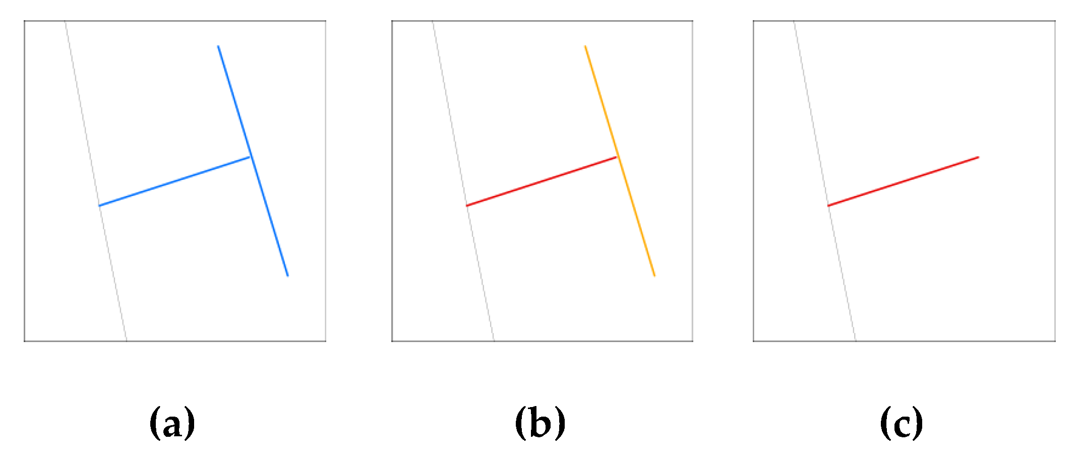
| L shape Portrait e.g., dimension parallel with shoreline smaller than the other (see Figure 11f and Figure 12a,b) L shape Landscape e.g., dimension parallel with shoreline larger than the other (see Figure 11g and Figure 12c,d) | Stage A Portrait: If MBR width < limit transform to single line If single line length (distance from coastline) > limit then portray else delete Landscape: If MBR length < limit transform to single line If single line length (distance from coastline) > limit then portray else delete Stage B If length (distance from coastline) < limit then delete | MBR: width medium or large. One segment in contact with coastline. Almost right angle between segments. Based on the azimuth of segments distinguish the two perpendicular lines and decide on structure orientation (landscape or portrait). For portrait use MBR width and for landscape use MBR length to decide on generalization. (MBR width is always the smaller dimension of the MBR and MBR length is always the larger dimension of the MBR). |
| Pi Shape (see Figure 11h and Figure 13) | Stage A If width < limit then collapse to single line If single line length (distance from coastline) > limit then portray else delete Update natural coastline Stage B If length (distance from coastline) < limit then delete | MBR: width medium. Can be drawn with one line. Two segments in contact with coastline. Based on azimuth of segments identify the lines transverse to the shoreline. Calculate the maximum and the minimum length of the line segments transverse to the coastline. Identify the minimum and the maximum line segments transverse to the coastline. Compute the distance between the maximum and the minimum transverse segments. This distance is the width that is critical for generalization. Identify the Pi Shape structure based on the fact there are only two transverse line segments. From the maximum transverse line create a new structure that will replace the original Pi Shape, when the width of the structure is too short according to the map scale specifications. Find natural coastline segments that are connected to the transverse lines. Extend the natural coastline segment associated with the minimum transverse line to the natural coastline segment associated with the maximum transverse line |
| Boot Shape (see Figure 11i and Figure 14) or T Shape (see Figure 11j and Figure 15) | Stage A If minimum transverse line length < limit then collapse this part to single line. If distance between transverse lines (width) < limit then collapse this part to single line. If single line length (distance form coastline) > limit then portray else delete Update natural coastline Stage B If length (distance from coastline) < limit then delete | MBR: width medium. Can be drawn with one line. Two segments in contact with coastline Based on azimuth of segments identify the lines transverse and parallel to the shoreline. Calculate the maximum length and the minimum length of the line segments transverse to the coastline. The minimum transverse line length is critical for the generalization. Compute the distance between the maximum and the next to minimum transverse segment. This distance (width) is critical for the generalization. Identify Boot Shape or T Shape structures based on the fact that there are more than one transverse segments that are smaller than the maximum value e.g., 2 (boot shape) or 3 (T Shape). Identify the minimum transverse segment (s), the maximum transverse segment, and the intermediate. Identify the maximum segment parallel to the shoreline (cup). When the minimum transverse segment is considered too small (<0.3 mm), then keep the maximum transverse line and the maximum of the transverse segments smaller than the maximum. Extend these segments up to the cup of the structure to create a new generalized structure. From the transverse line with the maximum length create a new structure that will replace the generalized structure when the width of the structure is too small according to the map scale specifications. Connect the natural coastline segment associated with the minimum length line with the natural coastline segment associated with the maximum length line |
| T Shape (no width) (see Figure 11k and Figure 16) | Stage A If width (cap) < limit then collapse to single line (axis) If single line (axis) length (distance from coastline) > limit then portray else delete Stage B If length (distance from coastline) < limit then delete | MBR: medium width. Cannot be drawn with one line. One segment in contact with coastline. Based on the segments azimuth, distinguish the line perpendicular to the shoreline (axis) and the line parallel to the shoreline (cap). Use cap width to decide on size in order to invoke collapse. From the perpendicular line (axis) create a new structure that will replace the original T shape. Delete the line parallel to the shoreline (cap). |
| Antenna Portrait shape (see Figure 11l and Figure 17) | Stage A If width (cap) < limit then collapse to single line (axis) If single line (axis) length (distance from coastline) > limit then portray else delete Stage B If length (distance from coastline) < limit then delete | MBR: medium width. Cannot be drawn with one line. One segment in contact with coastline Based on the segments azimuth, distinguish the line transverse to the shoreline (axis) and the lines parallel with the shoreline (caps). Use cap width to decide on size in order to invoke collapse. From the transverse line (axis) create a new structure that will replace the original T shape. Delete the line parallel to the shoreline (cap) |
| Antenna Landscape shape (see Figure 11m) and Complex cases (see Figure 11n) | If distance from coastline < limit then delete | Due to difficulty in distinguishing the two main directions in the Antenna Landscape structure, only the distance from shoreline parameter can be applied. |
Appendix C. Contours Generalization Procedure as Applied in the Case Study Utilizing ArcGIS Geoprocessing Tools
- Creation of a new full coverage DEM: gaps in the dataset are filled as described earlier utilizing the “Create TIN” tool. The new DEM is converted to a point cloud and projected to the chart coordinate reference system.
- Contours preprocessing and classification: specific depth contours are extracted from the full coverage DEM according to chart specifications. Depth contours are enriched with additional information needed for the next steps and classified (Figure 2).
- Aggregation and smoothing of open depth contours, neighboring simple peaks and related integer soundings: the double-buffering method is applied with a custom Model Builder model utilizing the “Buffer tool” and other geo-processing tools.
- Aggregation of (a) complex contours, neighboring peaks and related integer soundings or (b) neighboring closed contours from the same category and related integer soundings: a custom tool based on the “Aggregate Polygons” tool is applied. Selected soundings are converted to small polygons with the buffer tool in order to be utilized in the “Aggregate Polygons” tool. Other nautical chart features are used as aggregation barriers in order to avoid overlaps.
- Smoothing: this is performed with the PAEK (polynomial approximation with exponential kernel) algorithm. Smoothing tolerance is set by the user in relation to nautical chart scale and line granularity.
- Exaggeration: based on the “Buffer” tool, closed contours may be enlarged in order to accommodate the portrayal of the required sounding value.
- Omission: based on the “Select” tool, features can be selected according to their characteristics and the “Delete” tool is used for their omission.
- Overlaps correction: based on the “Erase” tool, contours are “erased” by dredged areas polygons in order to delete overlapping lines and polygons. The same procedure is applied to resolve overlaps with the coastline.
Table A2.
Values of parameters (in meters) utilized in the case study for depth contours generalization for each scale.
Table A2.
Values of parameters (in meters) utilized in the case study for depth contours generalization for each scale.
| 1:10 K | 1:20 K | 1: 40 K | 1:80 K | |
|---|---|---|---|---|
| Contours and soundings aggregation | 30–300 | |||
| Contours aggregation of | 60 | 120 | 240 | |
| Double Buffering | 10–30 | 15 | 15 | 120 |
| Simplification Polynomial Approximation with Exponential Kernel (PAEK) | 50–70 | 100 | - | - |
| Exaggeration: minimum width for closed contours | 30 | 60 | 120 | 240 |
References
- Peters, R.; LeDoux, H.; Meijers, M. A Voronoi-based approach to generating depth-contours for hydrographic charts. Mar. Geod. 2014, 37, 145–166. [Google Scholar] [CrossRef] [Green Version]
- White, S.A.; Parrish, C.E.; Calder, B.R.; Pe’Eri, S.; Rzhanov, Y. LIDAR-derived national shoreline: Empirical and stochastic uncertainty analyses. J. Coast. Res. 2011, 62, 62–74. [Google Scholar] [CrossRef]
- NOAA Shoreline Website. NOAA Continually Updated Shoreline Product (CUSP). Available online: https://shoreline.noaa.gov/data/datasheets/cusp.html (accessed on 15 October 2020).
- IHO (International Hydrographic Organization). Regulations of the IHO for International (INT) Charts and Chart Specifications of the IHO, 4.7.0 ed.; Publication S-4; International Hydrographic Organization: Monte Carlo, Monaco, 2017; p. 452. [Google Scholar]
- IHO (International Hydrographic Organization). IHO Transfer Standard for Digital Hydrographic Data, 3.1 ed.; S-57 Publication; IHO: Monte Carlo, Monaco, 2000. [Google Scholar]
- IHO (International Hydrographic Organization). Enc Validation Checks, 6.1.0 ed.; S-58 Publication; International Hydrographic Organization: Monte Carlo, Monaco, 2018. [Google Scholar]
- Skopeliti, A.; Stamou, L.; Tsoulos, L.; Pe’Eri, S. Generalization of soundings across scales: From DTM to harbour and approach nautical charts. ISPRS Int. J. Geoinf. 2020, 9, 693. [Google Scholar] [CrossRef]
- Guilbert, E.; Zhang, X. Generalisation of submarine features on nautical charts. ISPRS Ann. Photogramm. Remote Sens. Spat. Inf. Sci. 2012, I-2, 13–18. [Google Scholar] [CrossRef] [Green Version]
- Beard, K. Constraints on rule formation. In Map Generalization: Making Rules for Knowledge Representation; Buttenfield, B., McMaster, R.B., Eds.; Longman Scientific & Technical: London, UK, 1991; pp. 121–135. [Google Scholar]
- Ruas, A.; Plazanet, C. Strategies for automated generalization. In Advances in GIS research II, Proceedings of the 7th International Symposium on Spatial Data Handling, Delft, The Netherlands, 12–16 August 1996; Kraak, M., Molenaar, M., Fendel, E., Eds.; Taylor & Francis: London, UK, 1997; pp. 319–336. [Google Scholar]
- NOAA (National Oceanic and Atmospheric Administration). Nautical Chart Manual; Version 2018.2; U.S. Department of Commerce, Office of Coast Survey: Silver Spring, MD, USA, 2018; Volume 1.
- Nyberg, N.; Pe’eri, S.; Catoire, S.; Harmon, C. An overview of the NOAA ENC Re-Scheming Plan. Int. Hydrogr. Rev. 2021, 22, 7–21. [Google Scholar]
- Miao, D. Gradual Generalization of Nautical Chart Contours with a B-Spline Snake Method. Master’s Thesis, University of New Hampshire, Durham, NH, USA, 2014; p. 135. [Google Scholar]
- Guilbert, E. Multi-level representation of terrain features on a contour map. GeoInformatica 2012, 17, 301–324. [Google Scholar] [CrossRef] [Green Version]
- Zhang, X.; Guilbert, E. A multi-agent system approach for feature-driven generalization of isobathymetric line. In Advances in Cartography and GIScience; Springer: Berlin/Heidelberg, Germany, 2011; Volume 1, pp. 477–495. [Google Scholar]
- Guilbert, E. Feature-driven generalization of isobaths on nautical charts: A multi-agent system approach. Trans. GIS 2015, 20, 126–143. [Google Scholar] [CrossRef] [Green Version]
- Smith, S.M.; Alexander, L.; Armstrong, A.A. The navigation surface: A new database approach to creating multiple products from high-density surveys. Int. Hydrogr. Rev. 2002, 3, 2–16. [Google Scholar]
- Guilbert, E.; Lin, H. B-spline curve smoothing under position constraints for line generalisation. In Proceedings of the Fourteenth International Symposium on Advances in Geographic Information Systems, Arlington, VA, USA, 2006; pp. 3–10. [Google Scholar]
- Guilbert, E.; Saux, E. Cartographic generalisation of lines based on B-spline snake model. Int. J. Geogr. Inf. Sci. 2008, 22, 847–870. [Google Scholar] [CrossRef]
- Miao, D.; Calder, B. Gradual generalization of nautical chart contours with a cubic B-spline snake model. IEEE Oceans. 2013, 863, 1–7. [Google Scholar] [CrossRef]
- NOAA (National Oceanic and Atmospheric Administration). Rescheme Cook Book; Version 1.0.0; Pe’eri, S., Bartlett, M., Ence, C., Gomez, G., Castillo, J., Auclert, G., Chauvet, P., Eds.; National Oceanic and Atmospheric Administration: Silver Spring, MD, USA, 2019; p. 195.
- Douglas, D.H.; Peucker, T.K. Algorithms for the reduction of the number of points required to represent a digitized line or its caricature. Cartogr. Int. J. Geogr. Inf. Geovis. 1973, 10, 112–122. [Google Scholar] [CrossRef] [Green Version]
- de Berg, M.; van Kreveld, M.; Schirra, S. Topologically correct subdivision simplification using the bandwidth criterion. Cartogr. Geogr. Inf. Syst. 1998, 25, 243–257. [Google Scholar] [CrossRef]
- Li, Z.; Openshaw, S. Algorithms for automated line generalization1based on a natural principle of objective generalization. Int. J. Geogr. Inf. Syst. 1992, 6, 373–389. [Google Scholar] [CrossRef]
- Wang, Z.; Müller, J.-C. Line generalization based on analysis of shape characteristics. Cartogr. Geogr. Inf. Syst. 1998, 25, 3–15. [Google Scholar] [CrossRef]
- IHO (International Hydrographic Organization). Electronic Navigational Chart, Version 4.0.0, 1.0.0 ed.; Publication S 101; International Hydrographic Organization: Monte Carlo, Monaco, 2018; p. 86. [Google Scholar]
- Calder, B.R.; Mayer, L.A. Automatic processing of high-rate, high-density multibeam echosounder data. Geochem. Geophys. Geosyst. 2003, 4. [Google Scholar] [CrossRef]
- NOAA. Chart 12327. New York Harbor (1:40,000), 109th ed.; NOAA: Silver Spring, MD, USA, 2020.
- Rice, G.; Wyllie, K.; Brennan, R.; Koprowski, C.; Wolfskehl, S.; Burnett, Z. The National Bathymetric Source. In Proceedings of the Canadian Hydrographic Conference 2020, Quebec City, QC, Canada, 24–27 February 2020; Available online: https://hydrography.ca/wp-content/uploads/2020/04/29_Rice_CHC2020_The_National_Bathymetric_Source.pdf (accessed on 28 February 2021).
- Ai, T.; Zhou, Q.; Zhang, X.; Huang, Y.; Zhou, M. A simplification of ria coastline with geomorphologic characteristics pre-served. Mar. Geod. 2014, 37, 167–186. [Google Scholar] [CrossRef]
Figure 1.
Contours list of depths (in meters) at each of NOAA’s reschemed scales based on the ladder approach.
Figure 1.
Contours list of depths (in meters) at each of NOAA’s reschemed scales based on the ladder approach.

Figure 2.
Identification of each contour properties leads to structure recognition and supports the generalization procedure with specific operators.
Figure 2.
Identification of each contour properties leads to structure recognition and supports the generalization procedure with specific operators.

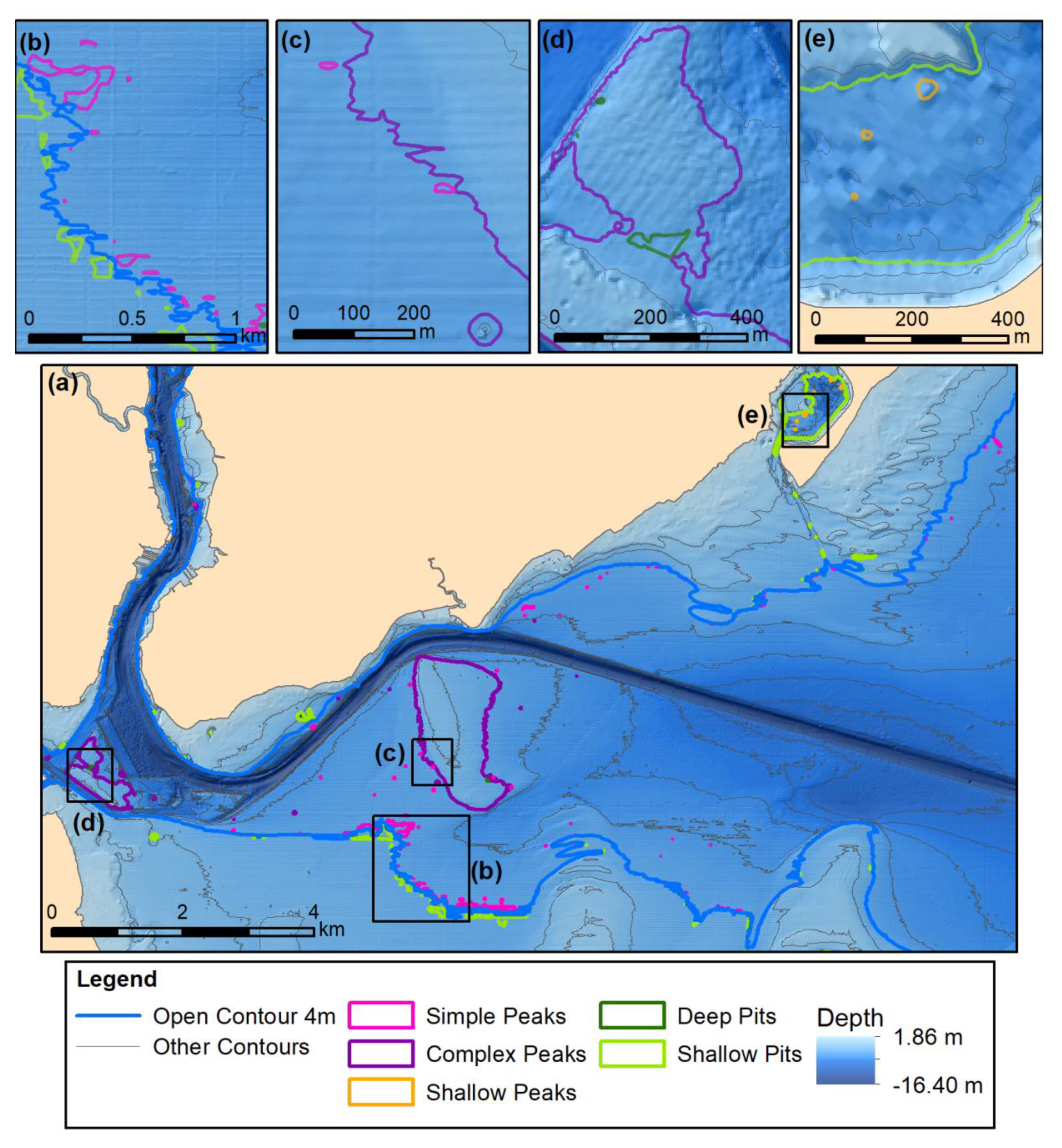
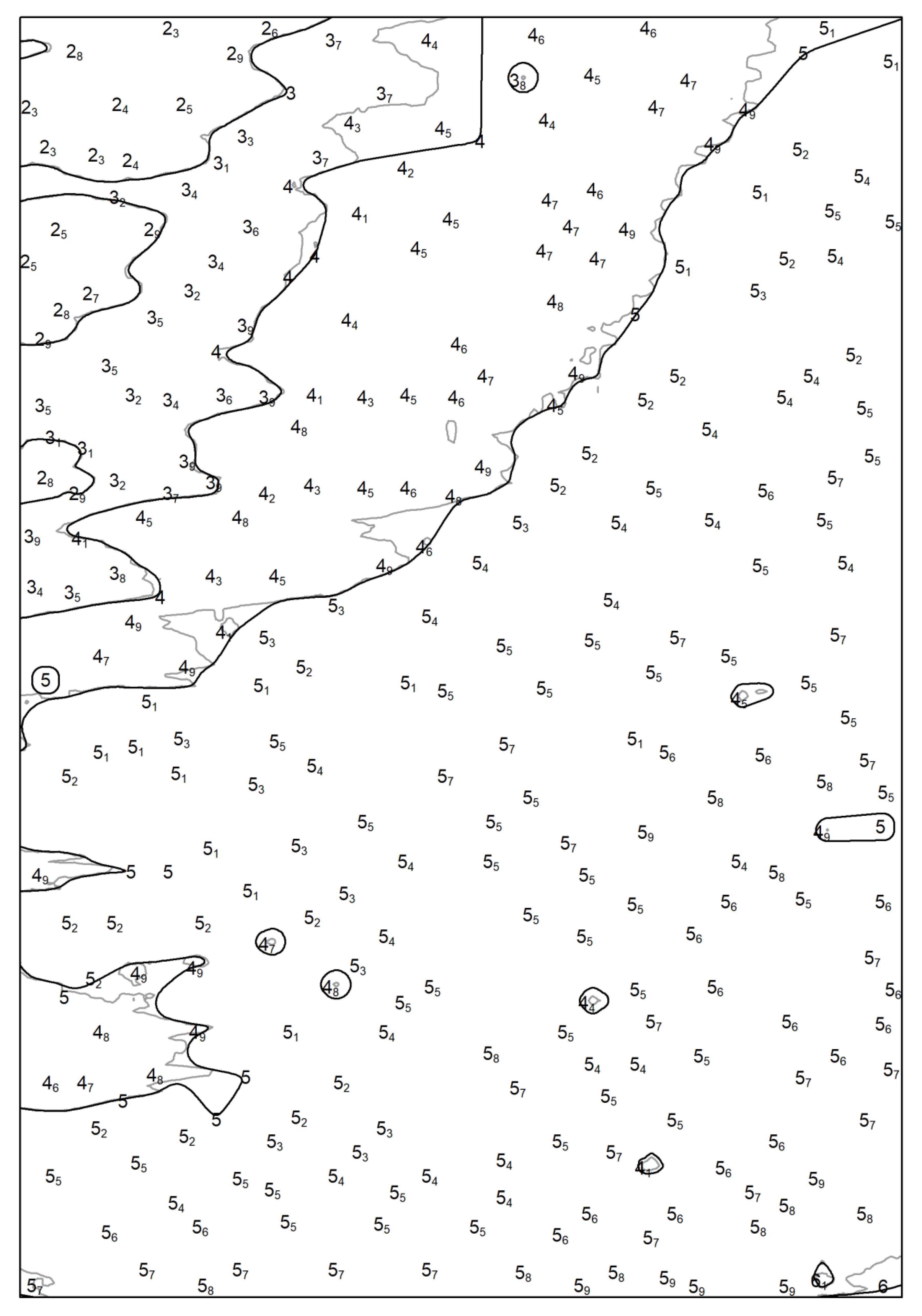
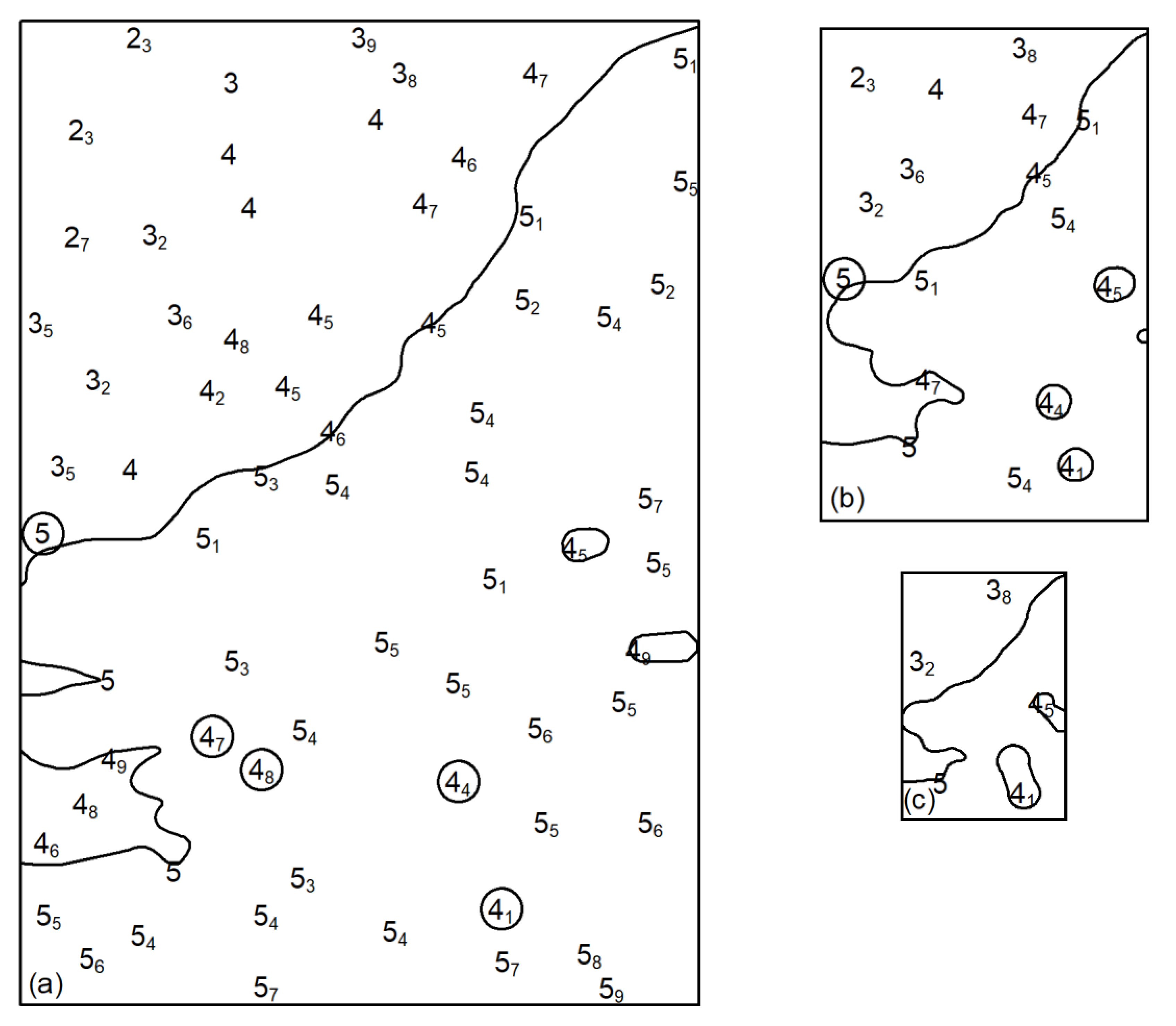
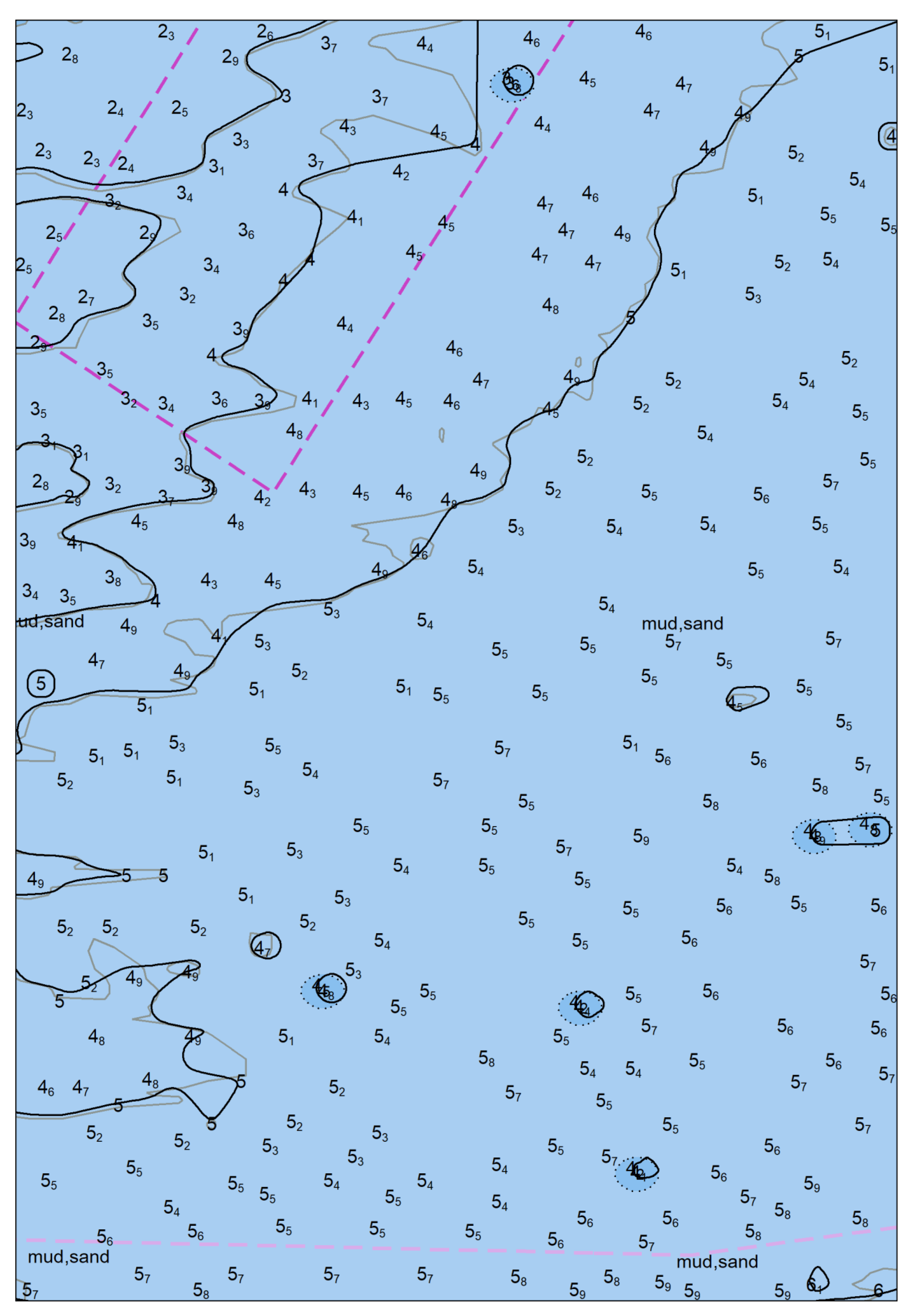
Figure 3.
Example of structure recognition for the 4m contour in the study area (Raw contours are portrayed) (a). Specific cases are portrayed in larger scales: Simple Peaks and the Open contour (b), Simple Peaks and Complex peaks (c), Complex Peaks and Deep Pits (d), Shallow Pits and Shallow Peaks (e).

Figure 4.
Aggregation of Simple Peaks and Open contours and Exaggeration of closed contours across scales: 2 m contour.
Figure 4.
Aggregation of Simple Peaks and Open contours and Exaggeration of closed contours across scales: 2 m contour.

Figure 5.
A number of soundings with depth value greater than 4 m e.g., 4.04, 4.06 etc., (a) are rounded to 4 m (b) according to the rounding specifications and thus they are not located within the 4 m depth contour. In order to ensure consistency, the 4 m depth contour (i.e., Open and Complex Peaks) should be shifted and forced to pass through the 4 m soundings and the closely located Simple Peaks (b).

Figure 6.
Sequence of operations for depth contour generalization.

Figure 7.
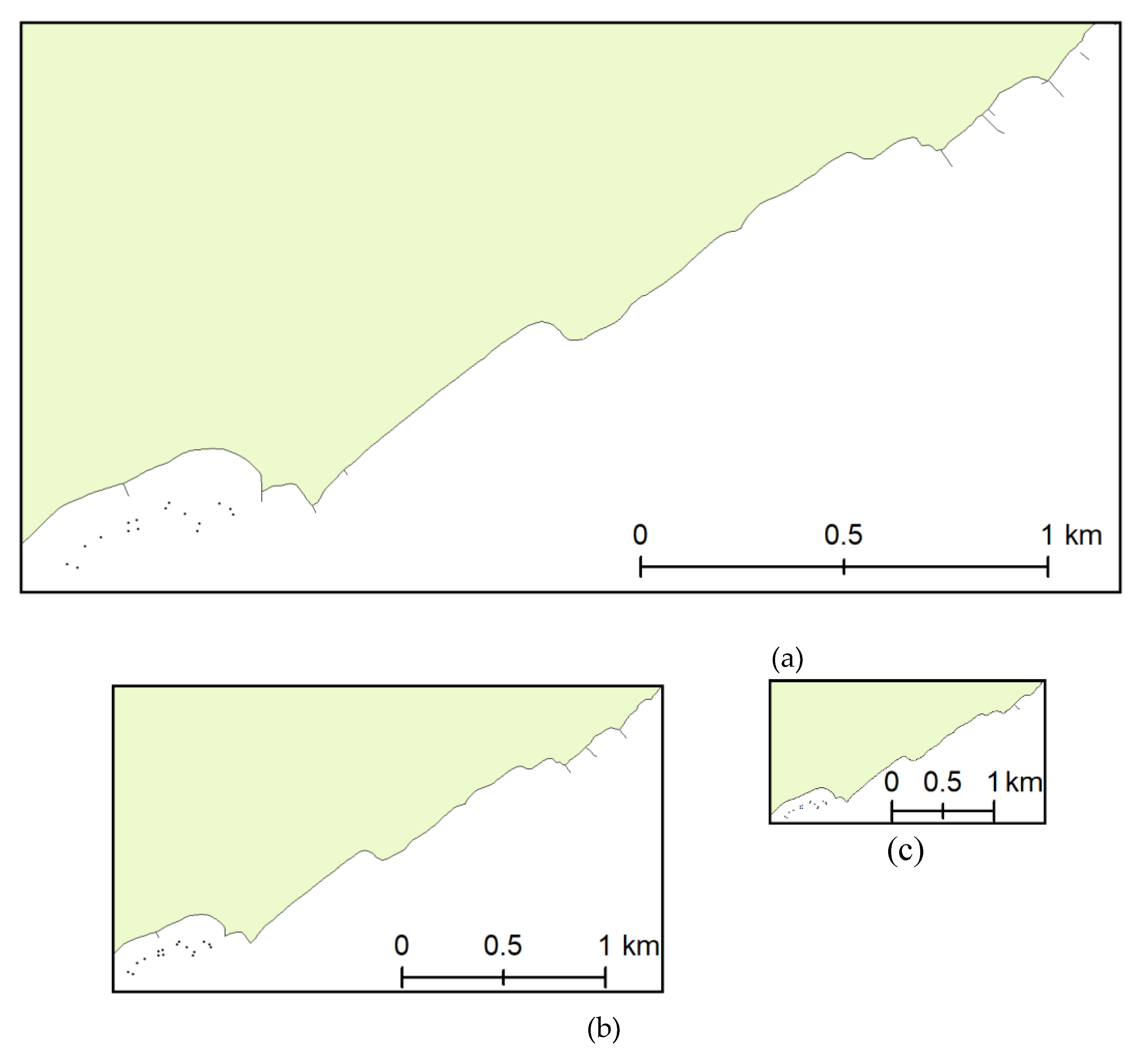
Islands located in proximity to the mainland coastline with respect to the chart compilation scale ((a)—yellow polygons) are aggregated to the coastline ((b)—green polygons) and a new coastline is formed (c).
Figure 7.
Islands located in proximity to the mainland coastline with respect to the chart compilation scale ((a)—yellow polygons) are aggregated to the coastline ((b)—green polygons) and a new coastline is formed (c).

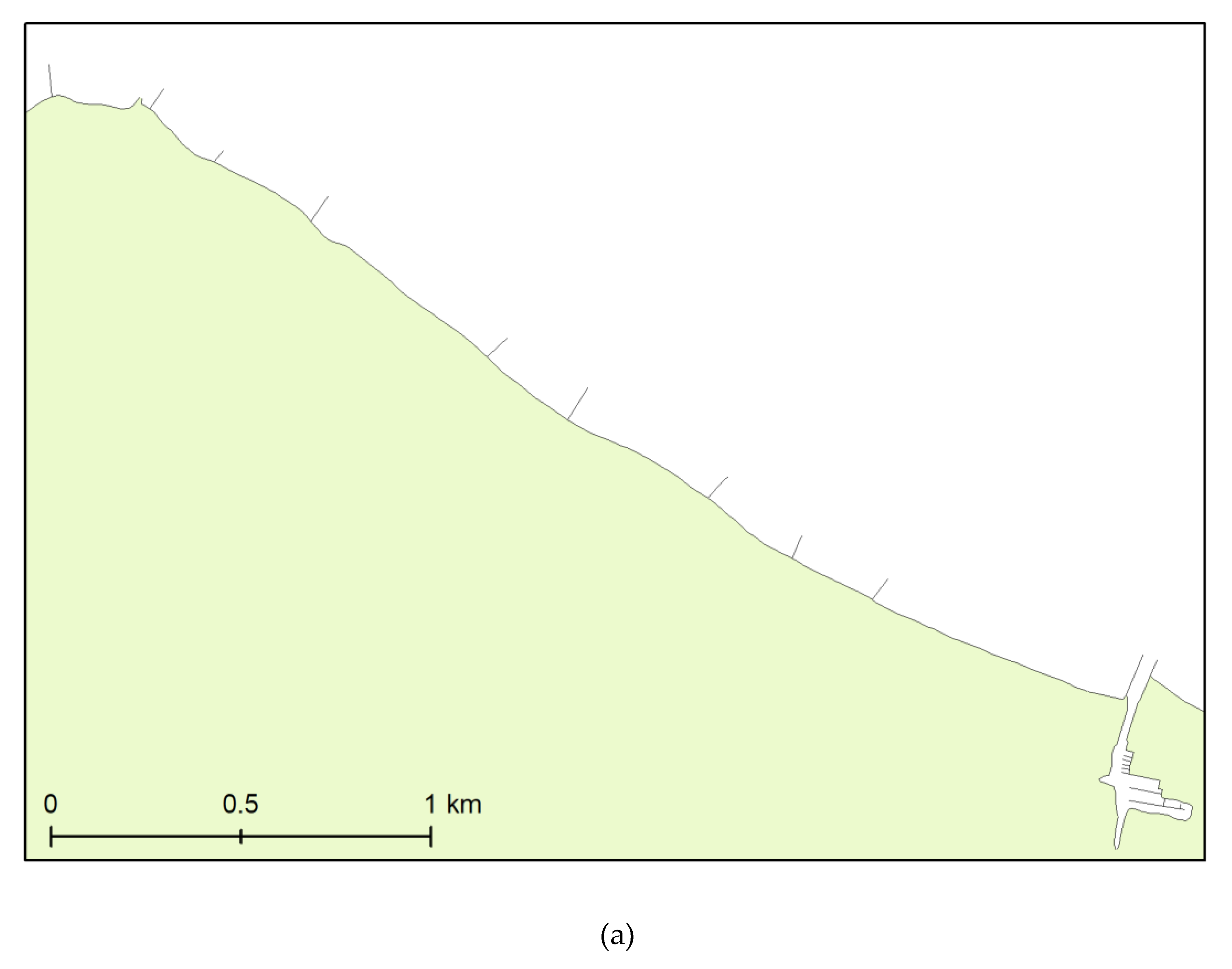
Figure 8.
Islets that are considered too small for the chart compilation scale (a), collapse to points (b).
Figure 8.
Islets that are considered too small for the chart compilation scale (a), collapse to points (b).

Figure 9.
Coastline polygons considered very narrow for the chart compilation scale (a), collapse to lines resulting from the polygon’s longer axis (b).
Figure 9.
Coastline polygons considered very narrow for the chart compilation scale (a), collapse to lines resulting from the polygon’s longer axis (b).

Figure 10.
Original natural coastline (a) is split into segments which are characterized in relation to the artificial coastline (red—cannot be deleted, green—can be deleted) (b), small segments are deleted according to scale specifications (see orange line overlaid on green line) (c), and the resulting line with appropriate vertex density (in blue ) is formed (d).

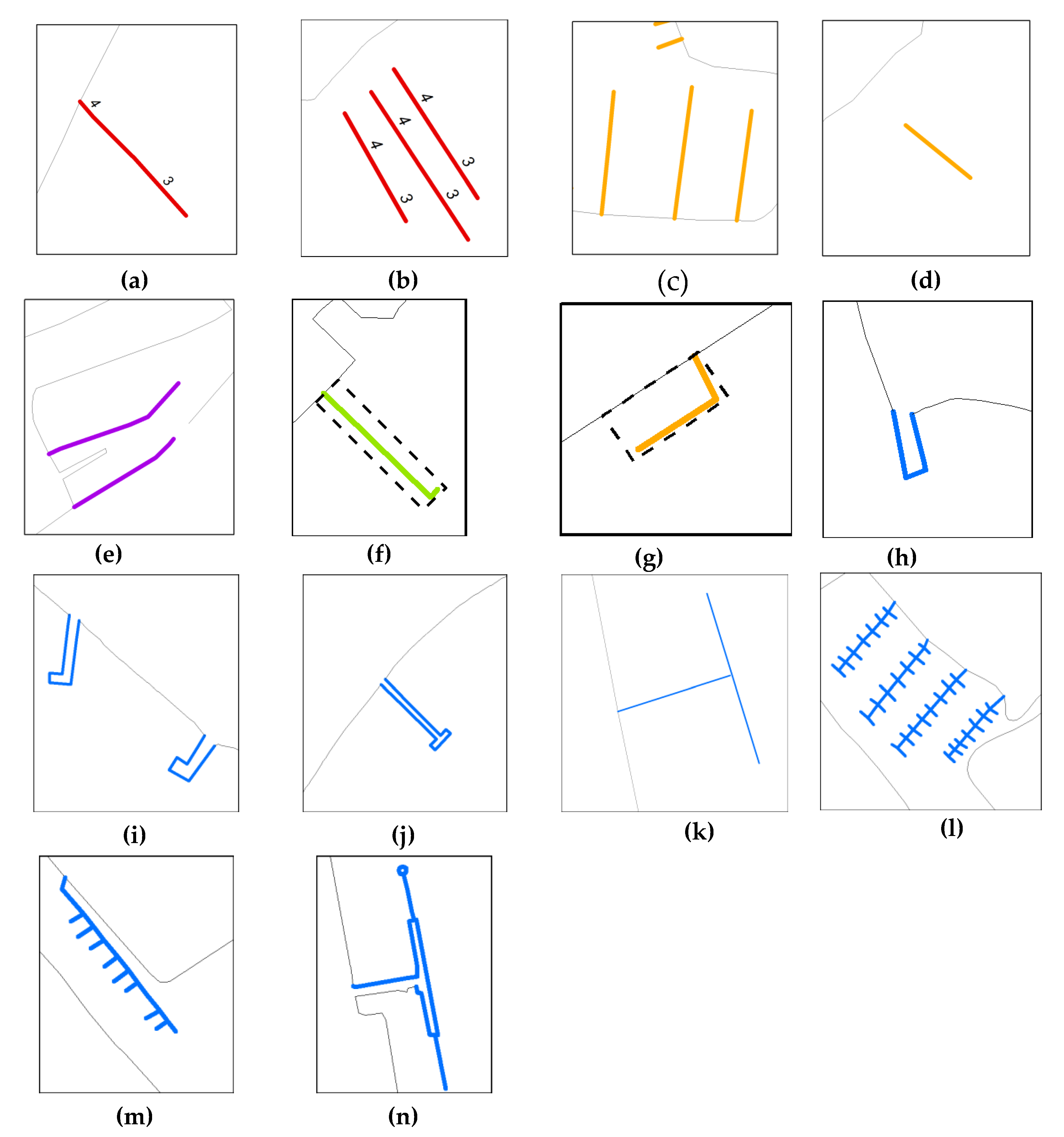
Figure 11.
Key artificial coastline features: (a) Line transverse and connected to shoreline—segments with different attributes e.g., Watlev, (b) Line transverse and not connected to shoreline—segments with different attributes, (c) Line transverse to and connected to shoreline—one segment, (d) Line transverse and not connected to shoreline—one segment, (e) Two segments with obtuse angle, (f) L-shape portrait e.g., dimension parallel with shoreline smaller than the other, (g) L-shape landscape e.g., dimension parallel with shoreline larger than the other, (h) Pi shape, (i) Boot shape, (j) T shape, (k) T shape (no width), (l) Antenna portrait shape, (m) Antenna landscape shape, (n) Complex cases.

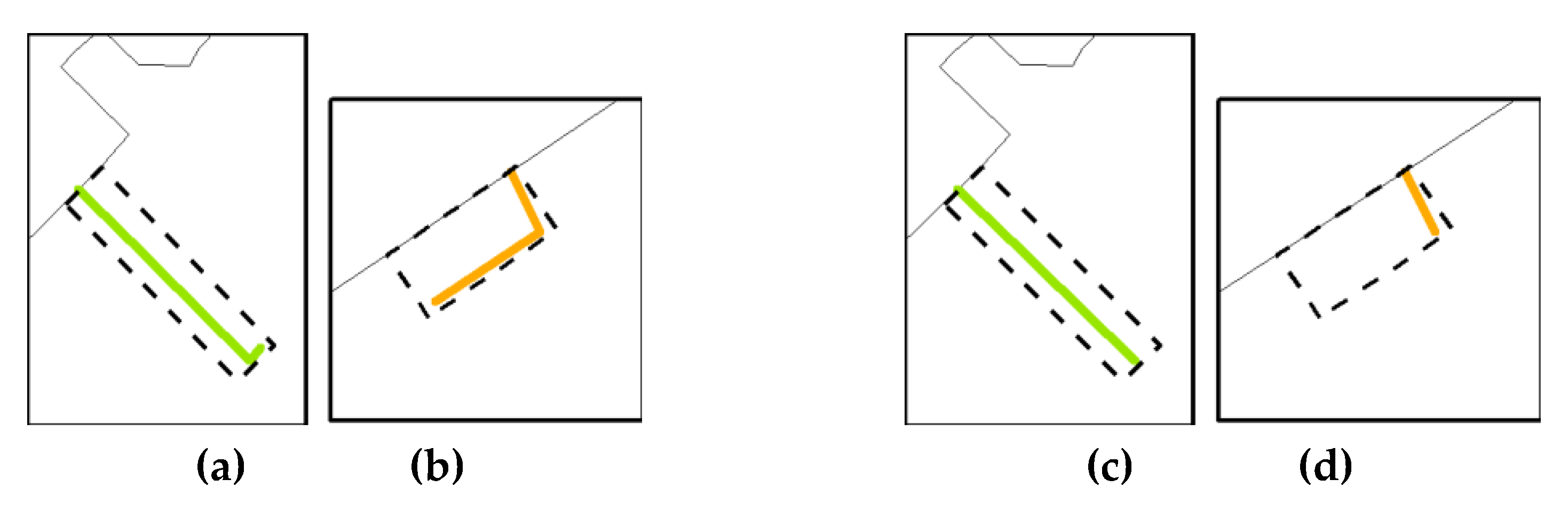
Figure 12.
L-shape generalization example (portrait: (a,b); landscape: (c,d)).

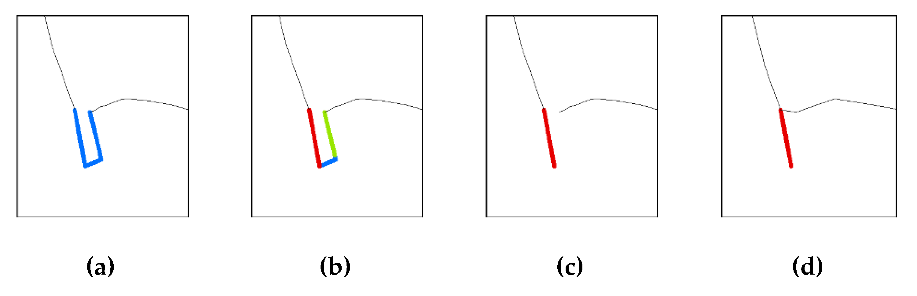
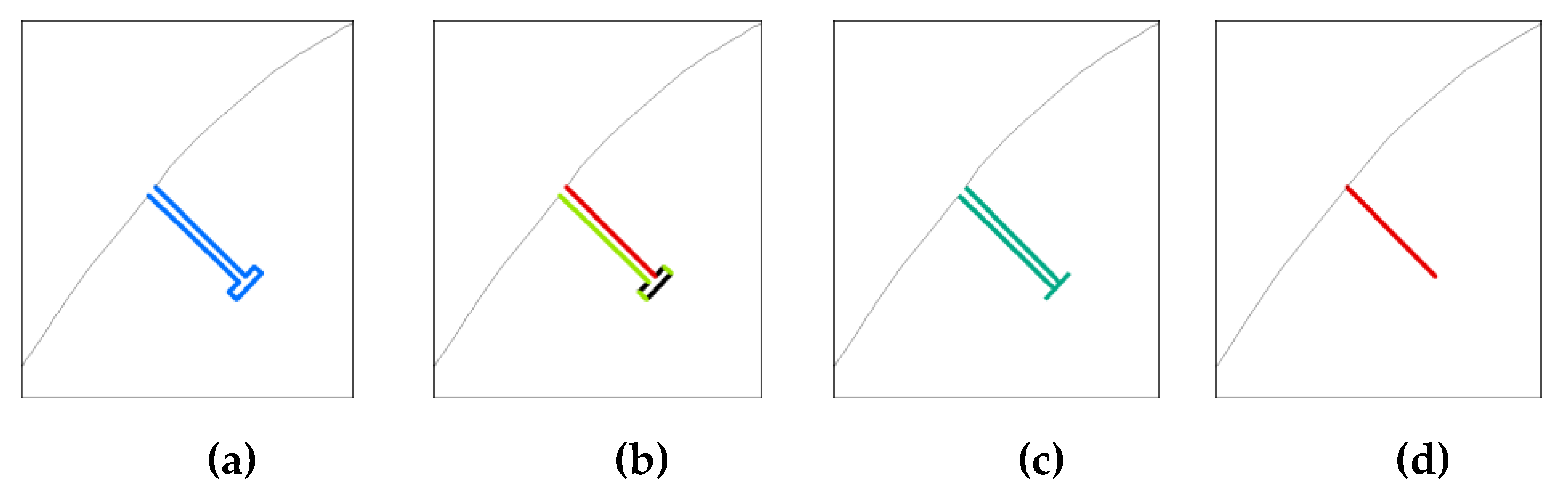
Figure 13.
Pi shape generalization example: (a) identify Pi-shape structure, (b) identify maximum transverse (red) and minimum transverse line (green), (c) keep maximum transverse line (red), and (d) extend natural coastline to fill the gap.
Figure 13.
Pi shape generalization example: (a) identify Pi-shape structure, (b) identify maximum transverse (red) and minimum transverse line (green), (c) keep maximum transverse line (red), and (d) extend natural coastline to fill the gap.

Figure 14.
Boot-shape generalization example: (a) identify boot shape structure, (b) identify the maximum transverse line (red), the shorter transverse lines (green) and the cups (black), (c) when the minimum transverse line is shorter than the limit set by the specifications, it is deleted. The shortest cup is deleted as well and the remaining transverse lines are extended to the larger cup. (d) When the width of the boot shape is thinner than the limit set by the specifications, only the maximum transverse line is kept and the natural coastline is extended to fill the gap.

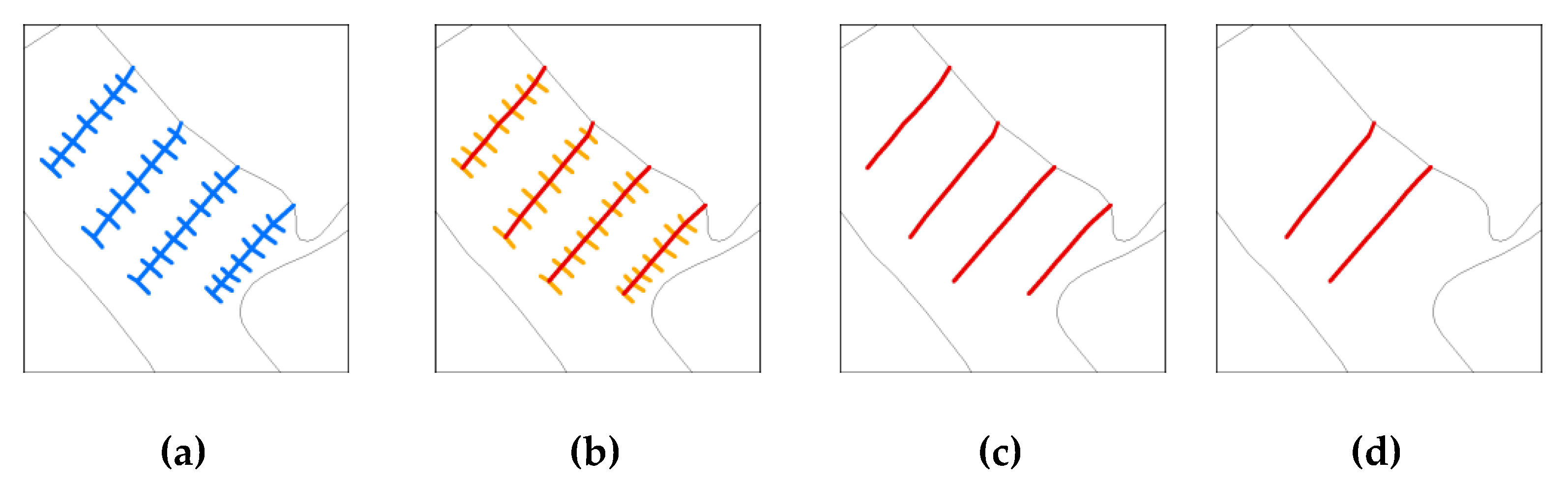
Figure 15.
T-shape generalization example: (a) identify T-shape structure, (b) identify the maximum transverse line (red), the shorter transverse lines (green) and the cups (black), (c) small transverse lines shorter than the threshold distance are deleted and the remaining transverse lines are extended to the cup, (d) if the width of a T-shape pier is thinner than threshold distance, then only the maximum transverse line is kept and the natural coastline is extended to fill the gap.

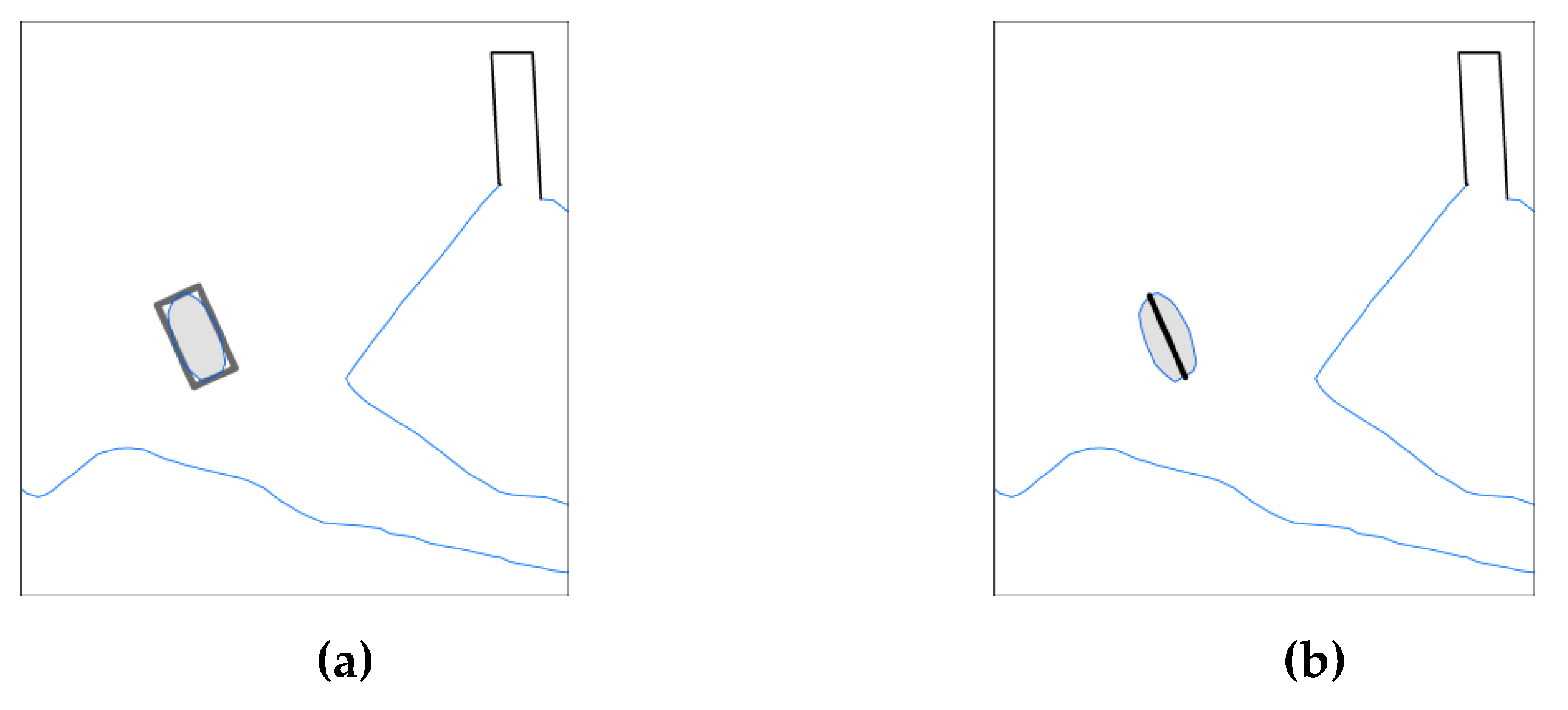
Figure 16.
T-shape (no width) generalization example: (a) identify T-shape structure, (b) identify transverse (red) line and cup (orange), (c) if the cup is shorter than the threshold distance then it is deleted.
Figure 16.
T-shape (no width) generalization example: (a) identify T-shape structure, (b) identify transverse (red) line and cup (orange), (c) if the cup is shorter than the threshold distance then it is deleted.

Figure 17.
Antenna shape generalization example: (a) identify antenna shape structure, (b) identify transverse (red) lines and cups (orange), (c) cup lines shorter than the threshold distance are deleted, and (d) transverse lines shorter than the threshold distance are deleted.
Figure 17.
Antenna shape generalization example: (a) identify antenna shape structure, (b) identify transverse (red) lines and cups (orange), (c) cup lines shorter than the threshold distance are deleted, and (d) transverse lines shorter than the threshold distance are deleted.

Figure 18.
Case study area (a) NOAA National Center for Environmental Information (NCEI) bathymetric data viewer, (b) NOAA digital elevation model (DEM) and the area covered by Figures 20, 21 and 24 (red box).
Figure 18.
Case study area (a) NOAA National Center for Environmental Information (NCEI) bathymetric data viewer, (b) NOAA digital elevation model (DEM) and the area covered by Figures 20, 21 and 24 (red box).

Figure 19.
Raw contours extracted from the full coverage DEM.

Figure 20.
Extract from the composed 1:10 K scale chart (contours 2, 3, 4, 5, 6, 7, 8, 10 m in black and raw contours as extracted from DEM in grey).
Figure 20.
Extract from the composed 1:10 K scale chart (contours 2, 3, 4, 5, 6, 7, 8, 10 m in black and raw contours as extracted from DEM in grey).

Figure 21.
Extracts from the composed charts: 1:20 K contours 2, 5, 10 m (a), 1:40 K contours 2, 5, 10 m (b) and 1:80 K contours 5, 10 m (c).
Figure 21.
Extracts from the composed charts: 1:20 K contours 2, 5, 10 m (a), 1:40 K contours 2, 5, 10 m (b) and 1:80 K contours 5, 10 m (c).

Figure 22.
Generalized coastline for scale 1:20 K (a), 1:40 K (b) and scale 1:80 K (c).

Figure 23.
Generalized coastline for scale 1:20 K (a), 1:40 K (b) and scale 1:80 K (c).


Figure 24.
Depth contours (in black) and soundings at 1:10 K scale are overlaid to an extract of NOAA electronic nautical chart (ENC) US5NYCBD (depth contours in gray).
Figure 24.
Depth contours (in black) and soundings at 1:10 K scale are overlaid to an extract of NOAA electronic nautical chart (ENC) US5NYCBD (depth contours in gray).

Publisher’s Note: MDPI stays neutral with regard to jurisdictional claims in published maps and institutional affiliations. |
© 2021 by the authors. Licensee MDPI, Basel, Switzerland. This article is an open access article distributed under the terms and conditions of the Creative Commons Attribution (CC BY) license (http://creativecommons.org/licenses/by/4.0/).
Share and Cite
MDPI and ACS Style
Skopeliti, A.; Tsoulos, L.; Pe’eri, S. Depth Contours and Coastline Generalization for Harbour and Approach Nautical Charts. ISPRS Int. J. Geo-Inf. 2021, 10, 197. https://doi.org/10.3390/ijgi10040197
AMA Style
Skopeliti A, Tsoulos L, Pe’eri S. Depth Contours and Coastline Generalization for Harbour and Approach Nautical Charts. ISPRS International Journal of Geo-Information. 2021; 10(4):197. https://doi.org/10.3390/ijgi10040197
Chicago/Turabian StyleSkopeliti, Andriani, Lysandros Tsoulos, and Shachak Pe’eri. 2021. "Depth Contours and Coastline Generalization for Harbour and Approach Nautical Charts" ISPRS International Journal of Geo-Information 10, no. 4: 197. https://doi.org/10.3390/ijgi10040197
Note that from the first issue of 2016, this journal uses article numbers instead of page numbers. See further details here.