
Abstract
Inverse problems are some of the most important mathematical problems in science and mathematics because their solution yields information about parameters that are not directly observable. Artificial neural networks have long been used as a mathematical modelling method and have been used successfully to solve inverse problems for application including denoising and medical image reconstruction. Many inverse problems result from integral processes that can be modelled using a linear formulation. These can be efficiently solved via simple networks which are easily trained with reasonable datasets. An innovative simple neural network architecture, the iterative linear neural network (ILNN), consisting of two non-hidden layer networks, one for the forward model and one for the inverse model, is proposed to solve linear inverse problems. Iteration between the two models refines network outcomes with greater accuracy than a network with only the inverse model. A training procedure accompanying the network is also introduced. The network needs to train only the inverse model with one-hot vectors as targets. The training inputs of the inverse model define the weights of the forward model. The number of targets is finite and equal to the length of the vector. With the defined targets, the training process ensures that the inverse model is at least a left inverse of the forward model. This leads to generalizable networks. The experimental results show that the ILNN produces good results even if its inverse model is not perfectly trained. The proposed network is applied to solve two linear inverse problems, deconvolution and the inverse Radon transform. The network successfully reconstructed original data following blurring and Radon transformation.
Export citation and abstract BibTeX RIS

Original content from this work may be used under the terms of the Creative Commons Attribution 4.0 licence. Any further distribution of this work must maintain attribution to the author(s) and the title of the work, journal citation and DOI.
1. Introduction
Inverse problems are encountered in many fields of science and engineering. The inverse theory deals with the development of tools to extract useful system parameters from physical measurements of system outputs. This is the inverse of the forward problem where the system output is predicted from system parameters. The fitting of a curve to experimental data, image reconstruction in x-ray computed tomography and remote sensing from satellite-borne systems are examples of the application of inverse theory.
Analytical techniques for solving inverse problems have a long history [1]. When using an analytical approach, the forward model is explicitly described, the criteria for obtaining a solution are decided, and a solution approach is chosen. Artificial Neural Networks (ANNs) have long been used as a mathematical modelling method [2, 3] and have recently shown outstanding performance on object classification and segmentation tasks [4, 5]. Motivated by these successes, researchers have begun to apply ANNs to the resolution of inverse problems such as denoising, deconvolution, super-resolution [6, 7], and medical image reconstruction [8–10].
Before solving real world problems, ANN parameters are learned from large data sets with pairs of sample inputs and outputs from corresponding forward models. As a result of the learning procedure, a direct mapping of outputs to inputs is obtained. To ensure that the network is not overfitting and successfully maps unseen data, training an ANN requires datasets of sufficient size and sophisticated training procedures, and is computationally expensive [4]. The difficulty of training ANNs is well known and many factors, including network architecture, activation functions used [11], the selection of training data [12–14] and the training method [15] can affect the results of training.
Despite these difficulties, ANNs have become popular because, by employing multiple layers and non-linear activation functions, they can be applied to non-linear problems. However, many inverse problems resulting from integral processes can be modelled by linear forms. These can be efficiently solved by simple networks which are easily trained using reasonable datasets. Simple networks having no hidden units and involving only input and output units have been used to solve many inverse problems, including Boolean functions, convolution integrals, Gaussian filtered images, edge-enhanced images and the Hough transform [16].
In this study, we confine our attention to linear inverse problems. We propose an iterative linear neural network (ILNN) comprising two simple networks to represent the forward and inverse models of investigated systems. The two models form an innovative closed feedback loop ANN architecture. The interaction between two models of the closed loop improves the accuracy of network outputs in comparison to that of networks having only inverse models. In company with the proposed network architecture, a training procedure with an artificial training dataset of predefined size is also introduced. The training data set is specifically created such that only the inverse model of the proposed network needs to be trained, and the parameters of the forward model can be directly obtained from the training set. The main advantages of the proposed network are (i) it does not need to be perfectly trained before yielding perfect results and (ii) with a defined training dataset, the inverse model is at least a left inverse of the forward model, ensuring the generalization of the proposed network.
2. Theory
2.1. Inverse problem
The objective of an inverse problem is to find the best model parameters  such that
  where
where  is the forward operator describing the explicit relationship between the observed data
  and the model parameters
In the case of a discrete linear inverse problem describing a linear system,  and
and  are represented as vectors, and the problem can be written as

where  is the observation matrix.
To solve for the model parameters, we might be able to invert the matrix  to directly convert the measurements into the model parameters. However, not all matrices are invertible. This is because we are not guaranteed to have enough information to uniquely determine the solution to the given equations unless we have independent measurements. From a linear algebra perspective, if the matrix
  is rank deficient, it is not invertible.
If the observation matrix cannot be directly inverted, methods from optimization theory are used to solve the inverse problem. To do so, we define an objective function for the inverse problem. This function measures how close the predicted data from the recovered model fits the observed data. The standard objective function is of the general form

which represents the  norm of the misfit between observed and predicted data from the model. The goal of the objective function is to minimize the difference between the predicted and observed data. As
  and
and  are given, the objective function is minimized by the proper selection of values of
  i.e.,
i.e.,

2.2. Deep neural network (DNN) and inverse problems
If observed data are corrupted by noise or missing, then the problem of equation (1) can become ill-posed and stabilization techniques referred as regularization methods must be applied to make the problem approximated by a well-posed problem. The methods consist of finding two functions: a data fidelity term  measuring the distance between
  and
and  and a regularization functional
  favouring appropriate minimizers or penalizing potential solutions with undesired structures. Instead of simply minimizing
  to fit
  to observed data, a weighted version is minimized

where  is the regularization parameter controlling the influence of the two terms on the minimizer.
The data fidelity term is often the squared norm distance in a Hilbert space as defined in equation (2). Regularization functionals can be either linear or non-linear and are application dependent. Popular functionals include Tikhonov regularization [17], the sparing regularization [18] and the total variation regularization [19]. For other regularization functionals and a comprehensive review of modern regularization methods, readers are referred to [20].
Recently, research in reverse problems has applied ANNs, particularly DNNs, to solve problems such as natural language processing, document analysis, face recognition, video analysis, failure prediction, information retrieval and handwriting and speech recognition [21–23]. Particularly in medical image reconstruction, several DNN models have been developed including automated transform by manifold approximation (AUTOMAP) [10], iCT-Net [24] and iRadonMAP [25]. In these models, there is at least one fully connected layer either at the input end (as in AUTOMAP and iRadonMAP) or at the output end (as in iCT-Net). This layer's purpose is to map observed data  to model parameter
  Other layers act as regularization constraints. As non-linear activation functions are used, the networks can mimic non-linear regularizations. Unlike analytic techniques, a priori regularization functionals do not need to be defined. The type of regularization depends on the training datasets and is specified during the process of training.
The role of DNN as a regularization constraint can be seen in deep image prior (DIP) introduced to solve inverse problems in an iterative manner, such as inpainting and computed tomography (CT) reconstruction [26, 27]. The approach is considered as a combination of data- and knowledge-driven modelling paradigms. It uses explicit knowledge-driven models when there are such available and learns models from example data using data-driven methods only when this is necessary. For example, in CT reconstruction using a U-Net network described in [27], the fully connected layer in AUTOMAP, iRadonMAP and iCT-Net is replaced by the forward model of the inverse CT problem that maps CT images to sinograms. The U-Net network provides a regularization constraint to obtain a stable solution. The output of the U-Net network is a CT image which is converted to a sinogram using the forward model before comparing to a desired sinogram. The discrepancy between sinograms is used to update network parameters for using in the next iteration.
2.3. Iterative linear neural network (ILNN)
We propose a method to solve linear inverse problems using linear neural networks. The proposed network has two simple linear networks to represent the forward model and the inverse model of investigated problems. In operation, the two models iteratively interact to improve outputs. Thus, we have named the proposed network an Iterative Linear Neural Network (ILNN). With a linear configuration, ILNN can be used to solve linear inverse problems with or without linear regularization such as the Tikhonov regularization. We show that the simple architecture of the proposed network makes it easily generalized with a suitable training set.
Each model of ILNN is a simple network which has two layers, an input layer and an output layer, and the activation function of the output layer is a linear function  The network does not have bias units and its input and output layers are connected by connections having different weights. The relationship between input
  and output
  of each model is mathematically represented by

where  is a matrix containing weight coefficients of the network connections.
Although equations (1) and (3) are of the same form, the way that  and
and  are obtained differs. The observation matrix
  in equation (1) is analytically derived whereas in neural network methods, element values of the weighting matrix
  in equation (3) are unknown and are estimated through a training process.
To ensure that the models in ILNN are inverses of each other, their inputs and outputs must have a reciprocal relationship as (i)  and (ii)
  where matrices
  and
and  are the weighting matrices of the forward and inverse models, respectively. Given a training set of vector pairs, each pair consisting of a target and a training input, the models are trained by adjusting element values of their weighting matrices to match model outputs to targets of corresponding training inputs, while at the same time, satisfying the reciprocal relationship.
Instead of training two models and checking the reciprocal relationship, we develop a training procedure with a customised training set so that only the inverse model needs to be trained and weighting coefficients of the forward model are directly determined from the training set. By carefully selecting the training set, we simplify the training process and ensure that the reciprocal relationship is satisfied.
Furthermore, the forward model of a linear inverse problem is a linear time-invariant (LTI) system that produces an output signal from any input signal subject to the constraints of linearity and time-invariance. The LTI system is completely characterized by its impulse response [28]. That is, for any input, the output can be calculated in terms of the input and the impulse response. The impulse response of a linear transformation is the image of Dirac's delta function under the transformation. We now show that if the proposed network is trained with a dataset generated from the impulse response of the forward model, the trained network has good generalization capability and is the generalized inverse of the forward model.
In our proposed approach, each target of the training set is a one-hot vector, which has only one nonzero element at a unique location, representing the Dirac's delta function. If the length of the vector is N then we will have N targets with different indices for the nonzero element covering the length of the vector. This ensures that all possible targets are fully covered by the smallest training set. As targets are inputs of the forward model, that means the domain of the forward model is fully covered in the training process. Furthermore, as each target is a one-hot vector with nonzero element at a unique location, the targets will equally distribute whole domain. It ensures that the trained network will avoid overfitting.
To train the inverse model, we provide a set of vector pairs  where
where is the target that the output of the inverse model must attain with corresponding input
  The training pairs
  are constructed based on the targets which are one-hot vectors or the Dirac's delta functions and the training inputs
  that are outputs of the forward operator
  applied on corresponding
  As
As  is the Dirac's delta function,
  is the impulse response of the forward model. We define the objective function of the inverse model as follows

The training process minimizes the objective function by adjusting the connecting weights 

We now show how, with the targets of one-hot vectors, values of the weighting matrix of the forward model can be obtained without training. Let  denote a target vector which has a nonzero element at the nth index and
  be the corresponding input of the inverse model. From the first condition of the reciprocal relationship, in the forward model these vectors must also be
  If all N targets are considered then the first condition can be written as

Since ![$\left[\underline{{x}_{0}}\ldots \underline{{x}_{N-1}}\right]$](https://content.cld.iop.org/journals/2399-6528/5/3/035008/revision3/jpcoabebcfieqn49.gif) is a unit matrix,
is a unit matrix, ![$G=\left[\underline{{y}_{0}}\ldots \underline{{y}_{N-1}}\right].$](https://content.cld.iop.org/journals/2399-6528/5/3/035008/revision3/jpcoabebcfieqn50.gif) As
As  is the weighting matrix of the forward model, it shows that the weights of the forward model are the training input of the inverse model
 ![$\left[\underline{{y}_{0}}\ldots \underline{{y}_{N-1}}\right].$](https://content.cld.iop.org/journals/2399-6528/5/3/035008/revision3/jpcoabebcfieqn52.gif)
As ![$G=\left[\underline{{y}_{0}}\ldots \underline{{y}_{N-1}}\right]$](https://content.cld.iop.org/journals/2399-6528/5/3/035008/revision3/jpcoabebcfieqn53.gif) satisfies the first condition of the reciprocal relationship, the training process of the inverse model is to find optimal weighting matrix
satisfies the first condition of the reciprocal relationship, the training process of the inverse model is to find optimal weighting matrix  to satisfy the second condition
  or
or

Thus to satisfy the reciprocal relationship the outcome of the training process is to make  a unit matrix or
  an inverse of
  In general,
  is not a square matrix. Its dimension is dependent on the lengths of
  and
and  If the lengths of
  and
and  are N and M, respectively, then dimension of
  is MxN. If
  is not a square matrix then
  with dimension NxM is not the inverse but a left inverse of
  [29]. It also shows that if a network is trained with the impulse response of the forward model of a linear inverse problem, then the trained network will be the generalised inverse, ensuring its generalization capability.
After defining  with the training input of the inverse model, the weighting matrix
  of the inverse model can be obtained by either taking the pseudo-inverse of
 or using a training process. If a noise free training set is used, then
  obtained from the training process will approximate the pseudo-inverse as least squares has been used as the objective function. To include the effect of noise on observed data, the inverse model can be trained against a dataset affected by noise. In this case,
  will be different from the pseudo-inverse of
  as the inverse model will learn the statistical distribution of noise from the training dataset and include it into model parameters
In practice, the training process is terminated when the difference between the training outputs and corresponding targets is less than a predefined value. As a result,  is an approximate of a unit matrix and it will affect to network outputs. To improve the output of the ILNN, the forward model
  and the inverse model
  are used iteratively.
The iterative refinement is adopted from an iterative method proposed in [30] for reducing the round off error in the computed solutions to systems of linear equations. At a particular iteration mth the iterative refinement can be mathematically described as follows.

It has been previously shown that this iterative process reduces errors and converges to the correct solution if H is an approximate inverse of G [30].
The architecture of the proposed ILNN is shown in figure 1. It differs from other multi-layer neural network architectures in which simple networks are cascade connected. In ILNN two models are connected to create a closed loop where the forward model acts as a feedback loop to improve the output of the inverse model through an iterative refinement process. After training, the network will operate as follows. Initially, the input and the output of the forward model are set to 0; input  is then fed into the inverse model to yield output
  The output of the inverse model is added to the input of the forward model to obtain a refined output. The refined output then becomes the input of the forward model, its output is subtracted from input
  and the residual is fed into to the inverse model. The output of the inverse model is then added to the previous refined output to obtain an updated refined output. The process is repeated several times until the desired refined output
  is obtained.

Figure 1. The architecture of the proposed iterative linear neural network (ILNN). The network consists of two linear networks, a Forward Model and an Inverse Model. Output of the Inverse Model is added to input of the Forward Model to obtain a refined output which is then input into the Forward Model. The output of the Forward Model is then subtracted from the input of the ILNN to obtain a residual that inputs into the Inverse Model.
Download figure:
Standard image High-resolution image3. Applications
We now demonstrate how the proposed network is trained and used to solve linear inverse problems. Two linear inverse problems, deconvolution and inverse Radon transform, inverse problems of convolution and the Radon transform, are considered. Convolution is defined as the integral of the product of two functions after one is reversed and shifted. The Radon transform takes a function defined on the plane to a function defined on the space of lines in the plane, with the value at a particular line being equal to the line integral of the function over that line. Both convolution and the Radon transform are integral transforms that can be modelled as linear problems. Their inverses are very important in image processing, particularly in medical imaging, where deconvolution is used to improve image resolution and the inverse Radon transform is used to reconstruct images from measured projections.
For each application, we evaluate the performance of the inverse model itself and that of ILNN, a combination of the inverse model and the forward model. Performance is also compared to other methods used in the field such as Wiener filtering in deconvolution and Filtered Back-Projection (FBP) and the fast iterative shrinkage/thresholding algorithm (FISTA) [31] for the inverse Radon transform.
The proposed network is implemented using the Python language and the TensorFlow library. In all applications, the inverse model of the network is trained with the Follow The (Proximally) Regularized Leader (FTRL) algorithm [32].
3.1. Deconvolution
The resolution of a measurement is always limited so that the recorded image of an object is completely dependent on the properties of the measurement device. Blurring arises if the signal intensity at any point in the image is the weighted sum of intensities from other points in object space. With detailed understanding of the weighting function, we can develop ways of correcting the image for the limitations of the measurement device. The transformation of information from a real object to a blurred image can be expressed mathematically using the operation of convolution. Deconvolution is the reverse operation which should be able to improve image quality. Deconvolution techniques are widely used in several fields [33, 34].
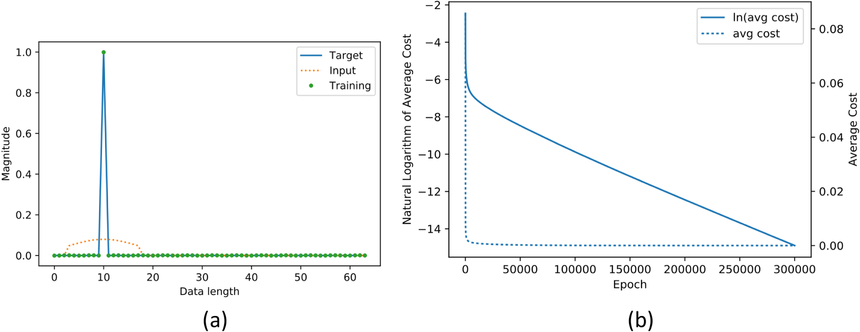
In this application, we show how to use ILNN to deconvolve a one-dimensional blurred signal to obtain a sharp original signal. The length of the input and output signal in this example is 64. As a result, the number of nodes of the input and output layers of the forward and inverse models is also 64. To train the inverse model, there are 64 one-hot vector targets each of length 64. To generate the training inputs, the targets are convolved with a Gaussian function with standard deviation 7 and length 15. Besides being used to train the inverse model, the training inputs are also the weights of the forward model.
The result of training is shown in figure 2. Figure 2(a) depicts a particular target (solid line) and the corresponding training input (dotted line). The inverse model is trained with a learning rate of 800 and 300 000 epochs. Figure 2(b) depicts the average training cost against number of epochs. It shows that the cost reduces very quickly in the first few thousand epochs and then plateaus. However, its natural logarithm shows that the cost continues to reduce gradually until training terminates at epoch 300 000 with an average cost of 9.07 × 10⁻⁸. The solid circle indicates that the training output is very close to the target (solid line) as shown in figure 2(a).

Figure 2. A training pair and training result with the average cost at different epochs. (a) A particular target (solid line), its convolution (dotted line) used as training input and training result (solid circle). (b) The average cost (dotted line) and its natural logarithm (solid line) at different epochs.
Download figure:
Standard image High-resolution imageTo evaluate the performance of the inverse model and of ILNN after training, we generated 100 sequences of random numbers of length 64 and convolved them with the same Gaussian function used in training. Figure 3 depicts one of the random sequences (dotted line) and its convolution (solid line), the network input. The output of the inverse model is shown as the symbol '+' in figure 3(a) and matches very well with the original random sequence.

Figure 3. One of random sequences used to evaluate the performance of the inverse model (a) and that of Wiener filtering (b). The random sequence (dotted line) is convolved with a Gaussian function to generate the input of the network and Wiener filter (solid line). The output of the inverse model and the filter is shown as the symbol '+'. Their output corresponds well with the original random sequence.
Download figure:
Standard image High-resolution imageThe performance of the proposed network is compared with that of Wiener filtering [34]. We set the additive correction factor of the Wiener filter to 0.0001 in this study. The result from Wiener filtering is depicted in figure 3(b). The output of Wiener filtering ('+' symbols) also matches the original sequence well.
Figure 4 depicts the difference between the outputs from the inverse model (dot dashed line), the ILNN after one iteration (solid line) and Wiener filtering (dotted line) with the original sequence shown in figure 3. The extremal difference between the inverse model and Wiener filtering with the original sequence was less than 0.004. However, the difference between the original sequence and the output of the proposed ILNN after one iteration is almost zero, smaller than that of the inverse model when iterative refinement is not applied.

Figure 4. The difference between output of the inverse model (dot dashed line), one iteration ILNN (solid line) and the Wiener filtering (dotted line) with the original random sequence shown in figure 3.
Download figure:
Standard image High-resolution imageThe mean squared error (MSE) of the output of Wiener filtering, the inverse model and ILNN (after one iteration) with the random sequences is given in table 1. With one iteration, the MSE of the ILNN is a thousand times smaller than that of the inverse model or Wiener filtering.
Table 1. The mean square error (MSE) of different methods testing with 100 random sequences.
| Method | Wiener filter | Inverse model | ILNN |
|---|---|---|---|
| MSE | 5.36 × 10⁻⁶ | 1.78 × 10⁻⁶ | 1.16 × 10⁻⁹ |
3.2. Inverse radon transform
Tomography is a non-invasive imaging technique that allows visualization of the internal structure of an object without the superposition of overlying and underlying structures that usually compromises conventional projection imaging methods. Tomography has found widespread application in many scientific fields, including physics, chemistry, astronomy, geophysics, and medicine [35, 36]. The Radon transform and its inverse provide the mathematical basis for reconstructing tomographic images from measured projection or scattering data.
The Radon transform offers a means of determining the total density of a certain continuous function  along a given line
  determined by an angle
  from the horizontal axis and a distance
  from the origin. The Radon transform of a two-dimensional image
  is defined as follows [37].

The two-dimensional Radon transform maps the spatial domain  to the Radon domain
  Each point in the Radon space corresponds to a straight line in the spatial domain. On the other hand, a point in the spatial domain is mapped to a sinusoid in the Radon space; hence Radon transform data is often called a sinogram.
Image reconstruction from Radon transform data is commonly known as image reconstruction from projections. An image can be reconstructed using the Inverse Radon transform [37]

The Inverse Radon transform can be expressed as the composition of two operators, the back-projection operator and the derivative filtering operator. The reconstruction algorithm of FBP is a direct implementation of the Inverse Radon transform formula with measured projections being filtered before they are back-projected [37].
The inverse Radon transform was previously approximated using a linear output network with a single hidden layer of sigmoidal nodes [38]. In this approach, network weight values were not obtained by a training process but were derived from an analytic solution. The same single-hidden layer neural network architecture with sigmoidal activation function has been evaluated in other applications including interpolating [39, 40] and matching of functions [41]. The non-linear sigmoidal activation function at the hidden layer allows the network to handle both linear and non-linear problems. However, it also makes training more difficult. It has been shown that there is no network that uniquely defines the underlying input/output relationship in both continuous and discrete domains [41]. The solution to a given problem usually employs an analytic approach to obtaining weight values or uses weights that are predefined in one layer and estimated in another [38, 39, 41].
As the Radon transform is an integral transform which can be expressed in a linear form, its inverse can be solved by a simple neural network without hidden layers. In this application, we demonstrate the use of ILNN to solve the inverse Radon transform problem. ILNN differs from the existing approaches described in [38, 39, 41] by taking advantage of the ability of neural networks to learn weights without knowledge of analytic solutions.
The inverse model in ILNN is trained and tested with images of dimension 64 by 64 and 100 Radon transform projections. This yields a sinogram of dimension 100 by 91. All measured data of images and their sinograms are flattened into one dimension before used in the network. As a result, the inverse model, which has the sinogram as input and an image as output, has 9100 nodes in the input layer and 4096 nodes in the output layer. For the forward model, the number of nodes in the input and output layers is equal that of the output and input layers of the inverse model, respectively.
To train the inverse model, we generate target images with zero background and a single pixel with value 1. The targets are then Radon transformed to obtain the corresponding sinograms. By appending each row two-dimensional data, target images are converted into one-hot vectors  of length 4096 and their sinograms are converted into training input vectors
  of length 9100. The total number of targets is 4096 which is the length of the target vector
  The training input vectors of the inverse model are used to determine the connecting weights of the forward model.
The result of training the inverse model is shown in figure 5. Figures 5(a) and (b) respectively depict one of the targets and its Radon transform prior to conversion to a one-dimensional vector. The inverse model is trained with the learning rate of 40 and 200 epochs. The training process is ended at epoch 200 with an average cost of 3.28 × 10⁻⁵. Figure 5(c) depicts the average cost and its natural logarithm at different epochs and shows that the cost converges to 0 smoothly.

Figure 5. One of training pairs and the average cost at different epochs. One of target images (a) and its Radon transform or sinogram (b). The dimensions of the target and its Radon transform are 64 × 64 and 100 × 91, respectively. The average cost (dotted line) and its natural logarithm (solid line) against number of epochs (c).
Download figure:
Standard image High-resolution imageTo evaluate the performance of the inverse model and of the proposed ILNN, we used 70,000 images in the MNIST (Modified National Institute of Standards and Technology) database of handwritten digits [42]. Many well-known machine learning algorithms have been tested on the MNIST database, facilitating the assessment of the relative performance of a novel algorithm [43]. Image intensities vary between 0 and 1 and the image dimensions are normalized to fit into a 28 by 28 pixel boundary box. For use with our trained model and network, image dimensions were scaled to 64 by 64 pixels. Figures 6(a) and (b) respectively depict an image in the MNIST database and its sinogram. Figures 6(c)–(f) show results of image reconstruction from the sinogram using FBP, FISTA with 500 iterations, the inverse model and ILNN after 50 iterations. The images differ, as demonstrated by the subtraction of each reconstructed image from the original image (figure 7). Figure 7(a) shows that the difference between the FBP image and the original image is largest at the object boundary. Figures 7(b) and (c) depict the difference between the original image and FISTA output and the output of the inverse model, respectively. Both differences are smaller and more evenly spread across the image space than the difference between the original image and the image reconstructed using FBP. After 50 iterations, the difference between the output of ILNN and the original image is smallest in comparison to the other two pairwise differences, as shown in figure 7(d).

Figure 6. One of MNIST images, its Radon transform and images reconstructed by different approaches. The original image with dimensions of 64 × 64 (a) and its Radon transform with 100 projections and dimensions of 100 × 91 (b). From the Radon transform data the image is reconstructed using the FBP approach (c), FISTA with 500 iterations (d), the inverse model (e) and the ILNN with 50 iterations (f).
Download figure:
Standard image High-resolution image
Figure 7. The differences between the original image and outputs of different approaches shown in figure 6 with the vertical bar indicating the range of differences. The difference between the original image and FBP output (min = −6.840 × 10⁻², max = 1.389 × 10⁻¹) (a) The difference between the original image and the output of FISTA after 500 iterations (min = −8.594 × 10⁻³, max = 8.121 × 10⁻³) (b) The difference between the original image and the output of the inverse model (min = −1.151 × 10⁻², max = 1.298 × 10⁻²) (c) The difference between the original image and the output of the ILNN after 50 iterations (min = −6.598 × 10⁻³, max = 6.560 × 10⁻³) (d) Values enclosed between round brackets are the minimum and maximum differences.
Download figure:
Standard image High-resolution imageFigures 8(a) and (b) depict the original image of the Shepp-Logan phantom and its Radon transform. The Shepp-Logan phantom is a standard test image [44] and is used widely by researchers in tomography [45]. The image has dimensions 64 by 64 and an intensity range of −10.933 to 274.648. Figure 8(c)–(f) display images reconstructed from the Radon transform data shown in figure 8(b) using FBP, FISTA, the inverse model and ILNN. Figure 9 shows the difference between the original phantom image and the outputs of the four different approaches. The difference with the output from FBP is largest and is most marked at the boundaries of the phantom (see figure 9(a)). Figures 9(b)–(d) depict the difference between the original phantom and the output of FISTA, the output of the inverse model and the output of the ILNN. Differences are small and spread more widely in the image space, particularly in the ILNN difference.

Figure 8. Image of Shepp-Logan phantom, its Radon transform and results of different image reconstruction approaches. The original phantom with dimensions of 64 × 64 (a), its Radon transform with 100 projections and dimensions of 100 × 91 (b), FBP result (c), output of FISTA with 500 iterations (d), output of the inverse model (e) and output of the ILNN with 50 iterations (f).
Download figure:
Standard image High-resolution image
Figure 9. The difference between the original phantom and outputs of different approaches shown in figure 8 with the vertical bar indicating the range of differences. (a) The difference between the original image and the result of FBP [minimum (min) and maximum (max) differences: min = −47.089, max = 77.941]. (b) The difference between the original image and the output of FISTA (min = −4.509, max = 4.347). (c) The difference between the original image and the output of the inverse model (min = −26.587, max = 27.031). (d) The difference between the original image and output of ILNN after 50 iterations (min = −2.507, max = 2.685).
Download figure:
Standard image High-resolution imageThe proposed method was tested on the LoDoPaB-CT dataset. The dataset is a benchmark dataset for low-dose CT reconstruction methods [46]. Figures 10(a) and (b) depict one of the dataset images and its Radon transform. The image has dimensions 362 by 362 and an intensity range of 0 to 0.5890. As the proposed network was trained with images of dimensions 64 by 64, it was scaled down to 64 by 64 before the Radon transform was taken. Figures 10(c)–(f) display images reconstructed from the Radon transform data shown in figure 10(b) using FBP, FISTA, the inverse model and ILNN. Figure 11 shows the difference between the original image and the outputs of the four different approaches. Like previous results, the difference with the output from FBP shown at figure 11(a) is largest and dominant at tissue boundaries. Figures 11(b)–(d) depict the difference between the original image and the output of FISTA, the output of the inverse model and the output of the ILNN. Differences are small and evenly spread across the image space.

Figure 10. One of images in LoDoPaB-CT dataset, its Radon transform and images reconstructed by different approaches. The original image with dimensions of 64 × 64 (a) and its Radon transform with 100 projections and dimensions of 100 × 91 (b). From the Radon transform data the image is reconstructed using the FBP approach (c), FISTA with 500 iterations (d), the inverse model (e) and the ILNN with 50 iterations (f).
Download figure:
Standard image High-resolution image
Figure 11. The differences between the original image and outputs of different approaches shown in figure 10 with the vertical bar indicating the range of differences. The difference between the original image and FBP output (min = −6.703 × 10⁻², max=8.940 × 10⁻²) (a). The difference between the original image and the output of FISTA after 500 iterations (min = −1.261 × 10⁻², max = 1.426 × 10⁻²) (b).The difference between the original image and the output of the inverse model (min = −2.001 × 10⁻², max = 2.194 × 10⁻²) (c). The difference between the original image and the output of the ILNN after 50 iterations (min = −1.147 × 10⁻², max = 1.240 × 10⁻²) (d). Values enclosed between round brackets are the minimum and maximum differences.
Download figure:
Standard image High-resolution imageTable 2 provides the MSE and extremal differences of the approaches shown in figure 7. Table 3 states the MSE between different approaches and 70,000 images in the MNIST database. Table 4 presents the MSE and extremal differences of different approaches shown in figure 9. The average MSE between different approaches and images in the LoDoPaB-CT dataset is provided in table 5. Table 6 gives the MSE and extremal differences of the approaches shown in figure 11. Contents of tables imply that the MSE of FBP is largest with significant differences at object boundaries, as seen in figures 7(a), 9(a) and 11(a). The MSE and the difference at object boundaries for FISTA and the inverse model are smaller than for FBP with FISTA outputs better than outputs of the inverse model. The smallest MSE is from ILNN with 50 iterations. The difference is not concentrated at boundaries but distributed throughout the image space, see figure 7(d), 9(d) and 11(d).
Table 2. MSE and extremal differences of different approaches for images shown in figure 7.
| Method | FBP | FISTA | Inverse model | ILNN |
|---|---|---|---|---|
| MSE | 1.210 × 10⁻⁴ | 7.263 × 10⁻⁷ | 3.719 × 10⁻⁶ | 3.584 × 10⁻⁷ |
| Minimum | −6.840 × 10⁻² | −8.594 × 10⁻³ | −1.151 × 10⁻² | −6.598 × 10⁻³ |
| Maximum | 1.389 × 10⁻¹ | 8.121 × 10⁻³ | 1.298 × 10⁻² | 6.560 × 10⁻³ |
Table 3. MSE of different approaches testing on MNIST database.
| Method | FBP | FISTA | Inverse model | ILNN |
|---|---|---|---|---|
| MSE | 1.926 × 10⁻⁴ | 1.995 × 10⁻⁶ | 1.067 × 10⁻⁵ | 1.018 × 10⁻⁶ |
Table 4. MSE and extremal differences of different approaches for images shown in figure 9.
| Method | FBP | FISTA | Inverse model | ILNN |
|---|---|---|---|---|
| MSE | 156.522 | 1.104 | 18.759 | 0.371 |
| Minimum | −47.089 | −4.509 | −26.587 | −2.507 |
| Maximum | 77.941 | 4.347 | 27.031 | 2.685 |
Table 5. MSE of different approaches testing on LoDoPaB-CT dataset.
| Method | FBP | FISTA | Inverse model | ILNN |
|---|---|---|---|---|
| MSE | 1.260 × 10⁻⁴ | 1.882 × 10⁻⁶ | 1.229 × 10⁻⁵ | 9.042 × 10⁻⁷ |
Table 6. MSE and extremal differences of different approaches for images shown in figure 11.
| Method | FBP | FISTA | Inverse model | ILNN |
|---|---|---|---|---|
| MSE | 1.560 × 10⁻⁴ | 2.817 × 10⁻⁶ | 1.567 × 10⁻⁵ | 1.413 × 10⁻⁶ |
| Minimum | −6.703 × 10⁻² | −1.261 × 10⁻² | −2.001 × 10⁻² | −1.147 × 10⁻² |
| Maximum | 8.940 × 10⁻² | 1.426 × 10⁻² | 2.194 × 10⁻² | 1.240 × 10⁻² |
3.3. Noisy deconvolution
To evaluate the performance of the proposed network in a noisy environment, the network was applied to deconvolve noisy data. The inverse model was trained with a training set generated from one-hot vectors as described in the Deconvolution application but training inputs were corrupted by random noise with maximum magnitude varying from 0.005 to 0.1. The model was trained with a learning rate of 800 and 300 000 epochs. To make the network learn the statistical distribution of random noise and not to memorise specific noise patterns, different random noise sequences were used in each training epoch. figure 12(a) depicts the training result of one of the targets. Under the effects of noise, it cannot perfectly match to the target as it can in the absence of noise as shown in figure 2(a). Figure 12(b) displays one of distorted inputs (dotted line) following the addition of random noise.

Figure 12. A training result and training pair used in the application to noisy deconvolution. (a) A particular target (solid line), its convolution corrupted by noise (dotted line) used as training input and training result after 300 000 epochs (solid circle). (b) A particular noise free convolved signal (solid line) and one of its distorted versions (dotted line) when a random noise with maximum magnitude of 0.075 is added.
Download figure:
Standard image High-resolution imageAfter training, the network was applied to deconvolve data corrupted by random noise. Figure 13(a) depicts an example noisy dataset (dotted line) used in the study. As the inverse model is trained with noisy inputs to learn the statistical distribution of noise from the training set, its weighting matrix is not an approximate inverse matrix of the forward model and iterative refinement will not reduce the difference between ILNN outputs and the true outputs. Figure 13(b) depicts the MSE between ILNN outputs and true outputs at different refinement iterations. The MSE increases as the number of iterations increases. However, at the first few iterations, the MSE reduces and reaches its minimum value at the iteration number referred as the optimal iteration. In this study, the optimal iteration is either 4 or 5.

Figure 13. Noisy test data and MSE of iterative refinement. (a) A particular noise free convolved signal (solid line) and one of its distorted versions (dotted line) used for testing when random noise with maximum magnitude of 0.075 is added. (b) MSE between network outputs and true outputs at different refinement iterations.
Download figure:
Standard image High-resolution imageFigure 14 depicts the output of deconvolution of the noisy signal shown in figure 13(a) using different approaches. Figures 14(a) and (b) show the output of the inverse model and ILNN after 4 refinement iterations, respectively. The result is stable and closely matches the true output, particularly for the ILNN with the optimal iteration. Figure 14(c) depicts the output of ILNN after 50 iterations and shows that the output is unstable as the number of iterations increases. For comparison, the same test set is deconvolved using the inverse matrix of the forward model and Wiener filtering. Figure 14(d) depicts the output of the inverse matrix (dotted line) and the output of Wiener filtering ('+') with the input of the noisy signal shown in figure 13(a). They are nearly identical and unstable. The output of ILNN with the inverse matrix is not included as the inverse matrix, which is analytically calculated, is not approximately but exactly inverse thus ILNN does not change the output of the inverse matrix.

Figure 14. Deconvolution using different approaches with true output (solid line). (a) Deconvolution using the inverse model. (b) Deconvolution using ILNN with the optimal iteration. (c) Deconvolution using ILNN with 50 iterations. (d) Deconvolution using the inverse matrix (dotted line) and Wiener filtering ('+').
Download figure:
Standard image High-resolution imageTable 7 shows MSE of different methods at different noise levels. Random noise with maximum magnitude varying from 0.005 to 0.1 is added to convolved signals. As a result, the signal-to-noise ratio (SNR) varies from 25.978 dB to −0.042 dB. There are 100 test sequences at each noise level and the tabulated MSE is the average value. The table shows that at high SNR (>20dB), the inverse matrix and Wiener filtering perform well with stable outputs and small MSE values. Their MSE is smaller than that of the inverse model at SNR larger than 20dB. However, as SNR decreases their outputs are unstable with MSE increasing. MSE of iterative refinements is smaller than that of the inverse matrix and Wiener filtering at all noise levels with the smallest MSE at the optimal iteration. By learning the noise distribution from the training set, the trained inverse model has regularization constraints in its weighting coefficients that make its output more stable than that of the inverse matrix and Wiener filtering. As shown in figure 14 with SNR of 2.456 dB, the output of the inverse matrix and Wiener filtering varies between −4 to 4 compared to 0 to 1 for the true output and the output of the trained inverse model.
Table 7. MSE of different methods testing with 100 random sequences.
| Noise Level | Mean squared error | |||||
|---|---|---|---|---|---|---|
| Max Magnitude | SNR (dB) | Inverse | Opt Refine | Refine | Inverse Matrix | Wiener |
| 0.0050 | 25.978 | 0.02938 | 0.00718 | 0.01490 | 0.01529 | 0.01605 |
| 0.0075 | 22.456 | 0.04269 | 0.01031 | 0.02754 | 0.03440 | 0.03612 |
| 0.0100 | 19.958 | 0.05355 | 0.01339 | 0.03605 | 0.06116 | 0.06421 |
| 0.0250 | 11.999 | 0.07929 | 0.03177 | 0.06703 | 0.38225 | 0.40143 |
| 0.0500 | 5.978 | 0.08590 | 0.05492 | 0.13575 | 1.52901 | 1.60589 |
| 0.0750 | 2.456 | 0.09599 | 0.07367 | 0.23131 | 3.44029 | 3.61337 |
| 0.1000 | −0.042 | 0.11499 | 0.10017 | 0.41907 | 6.11607 | 6.42387 |
4. Discussion
4.1. Simple network versus multi-layer network
One of advantages of neural networks is that their weights can be learned through a training procedure. However, an obvious drawback of the training procedure is that the objective function may contain local minima and optimization algorithms are not guaranteed to find a global minimum. Adding connections or extra hidden layers creates extra dimensions in weight space and these dimensions can provide paths around the barriers that lead to local minima in lower dimensional subspaces [47].
Multi-layer neural networks, including deep learning approaches, are used to solve complex problems but may sometimes exhibit unexplained behaviour. It is often difficult to formulate a heuristic basis for the solution obtained, potentially reducing trust in the networks [48]. Specific rules governing optimal network structure have not been defined and structures are generally devised from experience or through trial and error.
A number of issues should be addressed for efficient application of neural networks to a specific problem. These include selection of network type and architecture, the optimization algorithm and the method of countering overfitting. Overfitting of training data impairs the generalization properties of the model and results in untrustworthy performance when applied to novel measurements [15]. Complex models are much more prone to overfitting than simple models, implying that keeping the network architecture relatively simple should be an objective [49–51]. Large datasets do not guarantee good generalization properties [52].
Given the issues in training multi-layer networks, their use is inefficient if problems can be solved using simpler network. We have demonstrated that if inverse problems result from integral processes which can be modelled using a linear formulation then they can be efficiently solved with a simple network without hidden layers. Despite its simple architecture, the network has been used to compute Boolean functions, convolution integrals, Gaussian filtered images, edge-enhanced images and the Hough transform [16] where the network acts as an inverse model. The simple network can also represent both forward and inverse models of a linear problem. In the proposed ILNN there are two simple networks representing these two models and they interact such that the output of one network is the input of another to form a closed feedback loop. The experimental results show that the feedback interaction of two models makes the performance of the proposed network better than that of networks have only inverse models.
4.2. Optimal training data set of predefined size
A training set must be selected to ensure that the final network model generalizes well – that is, to achieve high performance on unseen data drawn from the same statistical population as the training data. To deal with this, targets representative of the whole population are required, potentially increasing the number of targets and lengthening the training process. Furthermore, even if the number of targets is large but they are not equally distributed, the network will tend to overfit where the targets are most concentrated. Optimal target selection avoids overfitting and reduces the size of the training set, without affecting generalization. Limiting the training size accelerates model training process.
In the proposed network, only the inverse model is trained with a training data set of predefined size. To train the inverse model, we generate a finite number of target and training input pairs. The targets are one-hot vectors and the number of training pairs equals the length of the target vectors. With this training data set the values of the weighting matrix of the forward model are fully defined and equal to the training input values. The value of weighting coefficients of the inverse model is obtained from a training process. As nonzero element of the one-hot vectors is at a unique location, all targets are different and with the smallest number, they cover and equally distribute whole target range. It ensures that the trained network has generalization capability and overfitting is avoided. The predefined size of the training set makes the proposed training procedure radically different from existing approaches in which training data are obtained from a database with number of samples as large as possible. Furthermore, it is customary to partition the available data into (at least) two sets, one to train networks and the other as a test set to measure the generalization capability of the trained networks. This partition may influence the performance of the trained network quite significantly [12]. In the proposed training procedure, we do not utilise a test set but generalization is ensured by the reciprocal relationship between the forward and inverse models. Even when the inverse model was trained with one-hot vectors as targets, our experimental results showed that the proposed network was able to successfully deconvolve blurred signals and reconstruct Radon transformed images.
4.3. Effect of optimization algorithms
Different optimization algorithms may perform better for simpler as opposed to larger neural network architecture and proper coupling of different optimization algorithms, network architectures and training methods is likely to be important. Several optimization algorithms available in the Tensorflow library, including the gradient descent, Adadelta [53], Adam [54], Adagrad [55], RMSProp and Ftrl [32] algorithms have been used to train the proposed inverse model. Gradient descent, Adadelta, Adagrad and Ftrl achieve similar convergence rates and can be used with a large learning rate (in the hundreds). Adam and RMSProp converge to zero cost with a small learning rate (<1). Figure 15 depicts the natural logarithm of the average cost of RMSProp, Ftrl and Adam in different epochs during the training of the inverse model for deconvolution. The results of other algorithms are similar to that of Ftrl and are not shown. The Adam algorithm has a fast convergence rate but is unstable. RMSProp has the largest average cost in comparison to the other algorithms. After 300,000 epochs, Ftrl has the smallest average cost (3.392 × 10⁻⁷). With the same number of epochs, the average cost of Adam and RMSProp are 1.564 × 10⁻⁶ and 2.056 × 10⁻⁴, respectively.

Figure 15. The natural logarithm of average cost at different epochs during training the inverse model for solving deconvolution problem using RMSProp with the learning rate of 0.05 (dash-dotted), Ftrl with the learning rate of 800 (solid) and Adam with the learning rate of 0.05 (dotted).
Download figure:
Standard image High-resolution image4.4. Effect of iterative refinement
The greatest advantage of the proposed method is that network performance is enhanced through a process of iteration so that outputs are accurate even though the inverse model is not perfectly trained. Figure 16(a) depicts the output of the inverse model after training using the RMSProp algorithm. As the average cost of the algorithm for complete training is large, the output of the inverse model is far from the original signal with a MSE of 0.2377. Iterative refinement improves the result and after 4 iterations, the MSE decreases to 2.787 × 10⁻¹¹. The output of ILNN (solid circle) shown in figure 16(a) matches the original signal (dotted line). Table 8 and figure 16(b) depict MSE between the original signal and the output of ILNN at different iterations; MSE reduces rapidly after a few iterations and even after the first iteration, it reduces considerably from 2.377 × 10⁻¹ to 7.801 × 10⁻⁴.

Figure 16. Signals and MSE with and without iteration for ILNN trained with the RMSProp algorithm. (a) The original random signal (dotted line), the convolved signal (solid line), the output of the inverse model ('+') and the output of the ILNN after 4 iterations (solid circle) are shown. (b) MSE between the output of the ILNN and the original signal at different iterations is shown.
Download figure:
Standard image High-resolution image
Table 8. MSE of the proposed network (trained with RMSProp algorithm) at different iterations
| Iteration | 0 | 1 | 2 | 3 | 4 |
| MSE | 2.377 × 10⁻¹ | 7.801 × 10⁻⁴ | 2.569 × 10⁻⁶ | 8.463 × 10⁻⁹ | 2.787 × 10⁻¹¹ |
4.5. Applications of ILNN
With a simple linear neural network architecture, ILNN can be used to solve linear inverse problems. It can also be used in linear problems with a linear regularization constraint such as the Tikhonov regularization to deal with noisy data. In this case, a dataset affected by noise is used for training. The network will learn the statistical distribution of noise from the training dataset and include it into network parameters.
The ILNN inverse model can replace the fully connected layer in DNNs such as AUTOMAP, iRadonMAP and iCT-Net. The layer is trained against the one-hot vector dataset before entire networks are learned with fixed parameters of the trained layer. This will constrain optimised solutions of network parameters to ensure trained networks are generalized. The entire networks could be trained against the one-hot vector dataset. However, to speed the training process, a larger set may be required and the one-hot vectors used as a test set to measure network generalization capacity.
The ILNN forward model can also replace analytic forward model used in DIP. In analytic approaches, a forward model is derived from the underlying physics and usually requires computing efforts. For example, in positron emission tomography (PET), CT and other volumetric ray tracing studies, to obtain the forward model or system response matrix, time-consuming ray-tracing calculations are required [56]. In ILNN, the system response matrix is simply a matrix with entries of the Radon transform of one-hot vectors or the impulse response of the CT forward system. This obviates complex computation.
Each approach has different advantages and disadvantages. The network architecture of ILNN is simple and it is easily trained to obtain generalization. However, it only solves linear inverse problems. DNNs with nonlinear activation functions can solve linear inverse problems with a wide range of regularizations. Their disadvantages are the requirement for large training datasets and the difficulty of proving the generalization of trained networks. In DIP approaches, generalization is irrelevant as their DNNs are not trained but used as a regularization constraint. However, they operate iteratively and recalculate network parameters for each observed datum and are thus computationally intensive.
The disadvantages of these approaches can be minimized if they work together, for example by combining them into a single approach with two networks connected in series. Here, the first network has an architecture like AUTOMAP with the ILNN inverse model as a fully connected layer and the second network has DIP architecture with the ILNN forward model. Only the first network is trained with the ILNN inverse model trained before the rest of the first network is trained. The trained ILNN inverse model acts as a generalization constraint of the first network. When unseen observed data input to the first network, the network generates outputs based on its trained parameters. The outputs are further enhanced by the second network. As the outputs of the first network are closed to solutions, the second network would need only a few iterations. Thus, the combination of approaches has the potential to increase the quality of outputs while reducing processing time.
5. Conclusion
We constructed an iterative linear neural network to solve linear inverse problems. The proposed network consisted of two simple linear networks, forward and inverse models, formed a closed feedback loop to refine network outcomes. By carefully selecting a training data set the training procedure was simplified without compromising generalization network properties. Only the inverse model required training and the weights of the forward model were directly obtained from the training set of the inverse model. We demonstrated that with targets of one-hot vectors and appropriate optimization algorithms, the training procedure had an optimal training set. The inverse model approximated the left inverse of the forward model ensuring that overfitting was avoided and the trained network is generalized.
The proposed network was applied to deconvolution and inverse Radon transform and generalization demonstrated. The network trained with one-hot vectors could reconstruct unseen original data and final results were improved through an iterative process making it robust against imperfect training of the inverse model. The network's performance was superior to that of Wiener filtering in deconvolution and FBP in the inverse Radon transform. It requires less number iterations than that of FISTA to achieve similar results.
Data availability statement
No new data were created or analysed in this study.