


Introduction
As snow transforms to ice it passes through an intermediate stage referred to as firn. According to Cuffey and Paterson (Reference Cuffey and Paterson2010), snow has density in the range 50–400 kg m−3, while firn has density in the range 400–800 kg m−3. The purpose of this paper is to model the elastic properties of dry snow and firn to help in monitoring the transition from snow to firn and then into ice. Measurements of elastic wave velocities provide a non-destructive method for estimating the mechanical properties, elastic moduli and density of snow and firn (Mellor, Reference Mellor1974; Shapiro and others, Reference Shapiro, Johnson, Sturm and Blaisdell1997). Smith (Reference Smith1965), for example, found a correlation between crushing strength and P-wave velocity for naturally compacted snow having densities in the range 390–914 kg m−3 from Camp Century on Greenland Ice Cap.
The mechanical properties of snow are of interest for a variety of applications such as construction on snow, snow removal, vehicle mobility and avalanche release and control (Salm, Reference Salm1982). The elastic properties relate stress and strain, and are needed for the interpretation of seismic measurements, which have been used to monitor and locate avalanches (Suriñach and others, Reference Suriñach, Vilajosana, Khazaradze, Biescas, Furdada and Vilaplana2005; Van Herwijnen and Schweizer, Reference Van Herwijnen and Schweizer2011; Lacroix and others, Reference Lacroix2012). Another application is the non-destructive estimation of density as a function of depth within compacting snow deposited on glaciers and ice sheets, as investigated by Schlegel and others (Reference Schlegel2019) using diving-wave refraction velocity analysis. This enables improved monitoring of the surface mass balance of glaciers and ice sheets using airborne or satellite altimetry by allowing the measured surface elevation over time to be corrected for compaction of snow.
Several authors (e.g. Pieritz and others, Reference Pieritz, Brzoska, Flin, Lesaffre and Coléou2004; Schneebeli, Reference Schneebeli2004; Srivastava and others, Reference Srivastava, Mahajan, Satyawali and Kumar2010; Köchle and Schneebeli, Reference Köchle and Schneebeli2014; Wautier and others, Reference Wautier, Geindreau and Flin2015; Srivastava and others, Reference Srivastava, Chandel, Mahajan and Pankaj2016; Gerling and others, Reference Gerling, Löwe and van Herwijnen2017) have used finite element analysis based on the 3-D microstructure of snow reconstructed from microtomography to predict elastic properties. This allows the relation between the computed elastic properties and parameters characterizing the microstructure such as porosity, the ratio of closed to total porosity, pore connectivity, pore surface-to-volume ratio and structure model index to be examined (e.g. Kaempfer and Schneebeli, Reference Kaempfer and Schneebeli2007; Ohser and others, Reference Ohser, Redenbach and Schladitz2009; Wang and Baker, Reference Wang and Baker2013; Gregory and others, Reference Gregory, Albert and Baker2014; Burr and others, Reference Burr2018; Fourteau and others, Reference Fourteau2019). For example, Srivastava and others (Reference Srivastava, Mahajan, Satyawali and Kumar2010) calculated the elastic properties of snow from microtomography using a voxel-based finite element technique, and compared the results with several microstructural parameters, the best correlation being with ice volume fraction.
The results of microtomography are limited to small samples. In contrast, elastic waves can be used to obtain a continuous measure of elastic properties over large depth intervals. Gerling and others (Reference Gerling, Löwe and van Herwijnen2017) showed that elastic moduli derived from finite element analysis using the 3-D microstructure of snow reconstructed from microtomography agreed with elastic moduli derived from elastic wave velocity measurements for snow under laboratory conditions.
Snow and firn are porous media consisting of a porous ice frame and pore space containing air. The propagation of elastic waves in porous media such as snow and firn may be treated using Biot theory (Biot, Reference Biot1956a, Reference Biot1956b, Johnson, Reference Johnson1982b; Sidler, Reference Sidler2015). This requires, as input, the density and elastic properties of air and the porous ice frame. The objective of this paper is to provide a method for computing the elastic properties of the ice frame in dry snow and firn using a physics-based approach that provides a consistent treatment of P- and S-velocities. The dynamic elastic properties are estimated using a modification of the differential effective medium scheme that accounts for the critical porosity ϕ c (Nur and others, Reference Nur, Mavko, Dvorkin and Galmudi1998) above which the bulk and shear moduli of the frame vanish.
Elastic wave velocities in snow and firn
Kohnen (Reference Kohnen1972) developed the following empirical relation between density and fast P-wave velocity based on measurements by Kohnen and Bentley (Reference Kohnen and Bentley1973) near New Byrd Station in West Antarctica:

where ρ(z) and V P(z) are the density and P-wave velocity at depth z, and ρ ice and V P,ice are the density and P-wave velocity of ice.
Diez and others (Reference Diez2014) gave a similar empirical relation between density and S-wave velocity based on measurements at Kohnen Station, West Antarctica:

where V S,ice and V S(z) are the S-wave velocity of ice and at depth z, respectively. Relationships between density and velocity such as those in Eqns (1) and (2) have the potential to provide improved monitoring of the surface mass balance of glaciers and ice sheets using airborne or satellite altimetry by allowing the measured surface elevation to be corrected for compaction of snow.
Since snow and firn are porous media, their elastic wave velocities may be calculated using Biot theory (Biot, Reference Biot1956a, Reference Biot1956b, Johnson, Reference Johnson1982b; Sidler, Reference Sidler2015). Denoting angular frequency by ω, fluid viscosity by η and fluid density by ρf, the crossover from low to high frequency behavior occurs at a frequency ωc at which the viscous skin depth, $\sqrt {2\eta /\rho _{\rm f}\omega }$ , is approximately equal to the pore radius, a, (Johnson, Reference Johnson, Burridge, Childress and Papanicolaou1982a):

Capelli and others (Reference Capelli, Kapil, Reiweger, Or and Schweizer2016) list pore diameters in snow in the range 0.2–0.35 mm. For air with η = 1.7 × 10⁻⁵ Pa s, ρ f = 1.3 kg m−3 (Sidler, Reference Sidler2015), Eqn (3) gives ωc < 3 kHz for this range of pore diameters.
At high frequency, this theory predicts that there is a fast compressional wave corresponding to the solid and fluid (air) moving in phase, a slow compressional wave corresponding to the solid and fluid moving out of phase, and one shear wave (Johnson, Reference Johnson, Burridge, Childress and Papanicolaou1982a). At low frequency, the fast compressional and shear waves propagate, but the slow wave is described by the solution of a diffusion equation. These predictions are consistent with observations of P-wave velocities that increase with density and are faster than in air when sources in direct contact with the ice frame are used, but that are slower than in air when sources not in contact with the ice frame are used (Capelli and others, Reference Capelli, Kapil, Reiweger, Or and Schweizer2016).
In the high frequency limit of the theory, the velocities of the fast and slow compressional wave and shear wave are given in the Appendix following Johnson (Reference Johnson, Burridge, Childress and Papanicolaou1982a). To illustrate the nature of these predictions, the empirical expressions for the required properties of snow as a function of porosity used by Sidler (Reference Sidler2015) based on prior information available in the literature are employed. Denoting porosity by ϕ, density and bulk modulus of the solid (ice) by ρs and K s, and bulk and shear moduli of the ice frame by K b and μb, the empirical relations used by Sidler (Reference Sidler2015) are as follows:


The following empirical relation for Poisson's ratio νb of the frame was used by Sidler (Reference Sidler2015):

Sidler (Reference Sidler2015) assumes a value K s = 10 GPa. Equation (5) then gives μ s = 2.61 GPa. An additional parameter required is a geometrical quantity τ > 1 that increases as the tortuosity of the pore space increases. Sidler (Reference Sidler2015) used the expression derived by Berryman (Reference Berryman1980a) for the case of isolated spherical solid particles in the fluid:

Figure 1(a) shows the predictions of Biot theory in the high frequency limit obtained using these expressions.
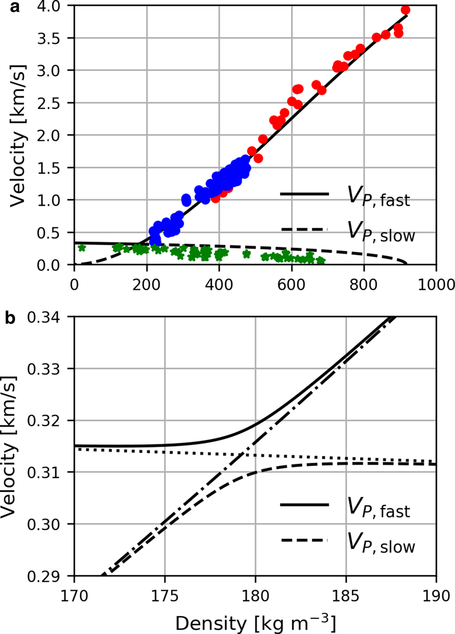
Fig. 1. Fast (full curve) and slow (dashed curve) P-wave velocities as a function of density as predicted by Biot theory. The circles in (a) show the data of Smith (Reference Smith1965) (red) and Yamada and others (Reference Yamada, Hasemi, Izumi and Sata1974) (blue), while the green stars show the data of Oura (Reference Oura1952), Ishida (Reference Ishida1965), Marco and others (Reference Marco, Buser, Villemain, Touvier and Revol1998) and Gudra and Najwer (Reference Gudra and Najwer2011). Panel (b) shows a detailed view of the fast and slow P-wave velocities for density in the range 170–190 kg m−3. The dash-dotted and dotted curves in (b) show the stiff frame predictions (K b, μ b ≫ K f).
Figure 1(b) shows a detailed view of the fast and slow P-wave velocities for density in the range 170–190 kg m−3, where the curves appear to cross in the upper subplot. The dash-dotted and dotted curves in the lower figure show the predictions of the theory in the stiff frame limit (K b, μ b ≫ K f, where K f is the bulk modulus of the fluid). The fast and slow P-velocities in this limit are given by Johnson (Reference Johnson, Burridge, Childress and Papanicolaou1982a) as:


A comparison of the fast and slow compressional velocities in Figure 1(b) with these expressions shows that at low density, when the ice frame has low bulk and shear moduli, the slow compressional wave travels mainly on the ice frame, while the fast compressional travels mostly in the air phase. At higher density, the fast compressional wave travels mostly on the ice frame, while the slow compressional wave travels mostly in the air phase. Above a density of 190 kg m−3 the fast wave is accurately represented by the stiff frame limit given by Eqn (8) which is essentially independent of τ because of the low density of air in comparison with that of ice.
The most complete published datasets with measurements of density, fast P- and S-velocities are those of Smith (Reference Smith1965) and Yamada and others (Reference Yamada, Hasemi, Izumi and Sata1974). The red and blue points in Figure 1(a) show these data, which are seen to be in reasonable agreement with the velocity of the fast compressional wave predicted by Biot theory using the empirical relationships of Sidler (Reference Sidler2015). The green stars show the data of Oura (Reference Oura1952), Ishida (Reference Ishida1965), Marco and others (Reference Marco, Buser, Villemain, Touvier and Revol1998) and Gudra and Najwer (Reference Gudra and Najwer2011). The data of Yamada and others (Reference Yamada, Hasemi, Izumi and Sata1974), Oura (Reference Oura1952), Ishida (Reference Ishida1965), Marco and others (Reference Marco, Buser, Villemain, Touvier and Revol1998) and Gudra and Najwer (Reference Gudra and Najwer2011) were taken from Capelli (Reference Capelli2021). It is seen that as density increases the green stars fall below the velocity of the slow compressional predicted by Biot theory using the parameters of Sidler (Reference Sidler2015). This suggests that τ is greater than that predicted by Eqn (7), and that the tortuosity of the pore space in snow and firn is greater than that assumed in deriving this equation. This is consistent with the observations of Schwander and others (Reference Schwander, Stauffer and Sigg1988) who found high tortuosity factors for firn samples, as compared to a sphere pack, indicating the existence of dead-end channels and/or relatively narrow passages in the pore channels. The absence of measurements of the slow wave at high density probably results from the high tortuosity of the pore space at high density.
Figure 2 compares the predictions of the empirical relations given by Eqns (1) and (2) with the measurements of Smith (Reference Smith1965) and Yamada and others (Reference Yamada, Hasemi, Izumi and Sata1974). The dotted curves correspond to P- and S-velocities V P,ice and V S,ice of ice estimated using density of ice of 915 kg m−3 given by Kohnen (Reference Kohnen1972) and bulk modulus K s = 8.90 GPa and shear modulus μ s = 3.46 GPa of isotropic polycrystalline ice calculated from the single crystal elastic stiffnesses of Gammon and others (Reference Gammon, Kiefte, Clouter and Denner1983) listed in Table 1 using the Hill (Reference Hill1952) average of the Voigt (Reference Voigt1910) and Reuss (Reference Reuss1929) bounds. The elastic moduli of Gammon and others (Reference Gammon, Kiefte, Clouter and Denner1983) were chosen for this comparison since these are the most recent measurements of the single crystal elastic stiffness coefficients of ice in Table 1. Also shown by the dash-dotted curves in Figure 2 are the predictions of Biot theory using the empirical relations of Sidler (Reference Sidler2015) listed above.

Fig. 2. Comparison between measurements of fast P-velocity (a) and S-velocity (b) in snow and firn measured by Smith (Reference Smith1965) (red points) and by Yamada and others (Reference Yamada, Hasemi, Izumi and Sata1974) (blue points) with fast P-velocity and S-velocity obtained using the empirical relations of Sidler (Reference Sidler2015) (dash-dotted curves). The dotted curves show the predictions of Eqns (1) and (2) with P- and S-velocities V P,ice and V S,ice of ice computed using a density of ice of 915 kg m−3 given by Kohnen (Reference Kohnen1972) and bulk modulus K = 8.90 GPa and shear modulus μ = 3.46 GPa of isotropic polycrystalline ice calculated from the single crystal elastic stiffnesses of Gammon and others (Reference Gammon, Kiefte, Clouter and Denner1983). The full curves show the predictions of Eqns (1) and (2) using a reduced shear modulus μ = 3.20 GPa for isotropic polycrystalline ice.
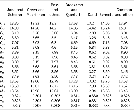
Table 1. Single crystal elastic stiffnesses (GPa) of ice measured by Jona and Scherrer (Reference Jona and Scherrer1952), Green and Mackinnon (Reference Green and Mackinnon1956), Bass and others (Reference Bass, Rossberg and Ziegler1957), Brockamp and Querfurth (Reference Brockamp and Querfurth1964), Dantl (Reference Dantl1968), Bennett (Reference Bennett1968) and Gammon and others (Reference Gammon, Kiefte, Clouter and Denner1983) compiled by Gusmeroli and others (Reference Gusmeroli, Pettit, Kennedy and Ritz2012) together with computed Voigt (V), Reuss (R) and Hill (H) estimates K V, K R, K H, μ V, μ R, μ H, M V, M R, M H, νV, νR and νH of the bulk K, shear μ and compressional M = K + 4μ/3 moduli and Poisson's ratio of an isotropic polycrystalline aggregate of ice crystals
It is seen in Figure 2(a) that Eqn (1) with bulk modulus of isotropic polycrystalline ice obtained from the single crystal elastic stiffnesses of Gammon and others (Reference Gammon, Kiefte, Clouter and Denner1983) agrees best with the measurements of Smith (Reference Smith1965), while the fast P-velocity obtained using the empirical relations of Sidler (Reference Sidler2015) agree best with the measurements of Yamada and others (Reference Yamada, Hasemi, Izumi and Sata1974). Figure 2(b) shows that Eqn (2) with shear modulus μ s = 3.46 GPa of isotropic polycrystalline ice obtained from the single crystal elastic stiffnesses of Gammon and others (Reference Gammon, Kiefte, Clouter and Denner1983) overestimates the measured S-velocities, while Biot theory using the empirical relations of Sidler (Reference Sidler2015) underestimates the S-velocities at high density. The shear modulus at zero porosity calculated from Eqns (4) and (5) used by Sidler (Reference Sidler2015) is μ s = 2.61 GPa, which is significantly less than any of the shear moduli for isotropic polycrystalline ice given in Table 1. The full curve in Figure 2(b) shows the prediction of Eqn (2) for a shear modulus μ s = 3.20 GPa. At high density, this is seen to give a much better prediction than that calculated from the data of Gammon and others (Reference Gammon, Kiefte, Clouter and Denner1983) and is the value used in the rest of this paper.
Poisson's ratio ν may be calculated from V P and V S as follows:

Figure 3 compares Poisson's ratio ν as a function of fast compressional velocity computed by combining Eqns (1) and (2) using bulk modulus K s = 8.90 GPa and shear modulus μ s = 3.46 GPa of isotropic polycrystalline ice calculated from the single crystal elastic stiffnesses of Gammon and others (Reference Gammon, Kiefte, Clouter and Denner1983) (dotted curve) and by using the empirical relation of Sidler (Reference Sidler2015) given by Eqn (6) (dash-dotted curve). The full curve shows the predictions of Eqns (1) and (2) using a reduced shear modulus μ = 3.20 GPa for isotropic polycrystalline ice. It is seen that Eqns (1) and (2) may lead to very small and even negative values of Poisson's ratio at low density, while ν > 0 for isotropic materials. The scatter in Poisson's ratio in Figure 3 is much greater than that in the velocities in Figure 2 as is expected from Eqn (10). As an example, Christensen (Reference Christensen1996) notes that an error of over $9 \percnt$ in Poisson's ratio can result from errors of $2 \percnt$
 in both V P and V S. For this reason, Poisson's ratio calculated from the measurements of Yamada and others (Reference Yamada, Hasemi, Izumi and Sata1974) are not shown in Figure 3, since V P and V S for this dataset were digitized from the plots in Yamada and others (Reference Yamada, Hasemi, Izumi and Sata1974) so that the errors in V P and V S are presumably greater than in the original measurements.
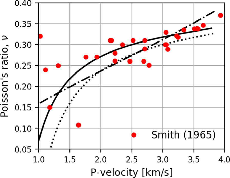
Fig. 3. Poisson's ratio calculated by combining Eqns (1) and (2) and from the empirical relation of Sidler given by Eqn (6) (dash-dotted curve) compared with that calculated from the measurements of Smith (Reference Smith1965) (red points). The dotted curves show the predictions of Eqns (1) and (2) with P- and S-velocities V P,ice and V S,ice of ice computed using a density of ice of 915 kg m−3 given by Kohnen (Reference Kohnen1972) and bulk modulus K = 8.90 GPa and shear modulus μ = 3.46 GPa of isotropic polycrystalline ice calculated from the single crystal elastic stiffnesses of Gammon and others (Reference Gammon, Kiefte, Clouter and Denner1983). The full curve shows the prediction of Eqn (2) using a reduced shear modulus μ = 3.20 GPa of isotropic polycrystalline ice.
Although the empirical fits of Sidler (Reference Sidler2015), Kohnen (Reference Kohnen1972) and Diez and others (Reference Diez2014) give a reasonable description of the data over the porosity range for which they were calibrated, they do not provide much insight into the underlying mechanisms for such relations. For example, it is not clear how to modify such relations to investigate the role of anisotropy, pore shape, etc. In contrast, a physics-based approach allows variations in anisotropy, pore shape, etc. to be investigated. In the following section, one possible physics-based approach is introduced and compared with the measurements of Smith (Reference Smith1965) and Yamada and others (Reference Yamada, Hasemi, Izumi and Sata1974) plotted in Figure 2.
Theoretical approach
To estimate the bulk and shear moduli of the porous ice frame, the differential effective medium scheme will be used. This has been reviewed, for example, by Norris (Reference Norris1985) and Zimmerman (Reference Zimmerman1990), and has been used widely to estimate the elastic properties of porous media with interconnected pore space such as porous sandstones (e.g. Zimmerman, Reference Zimmerman1990; Berge and others, Reference Berge, Berryman and Bonner1993; Berryman, Reference Berryman2004; Li and Zhang, Reference Li and Zhang2010).
Consider a two phase medium with bulk and shear moduli of phase i =1, 2 denoted by K i and μ i. In the differential effective medium scheme the effective elastic properties of the medium are modeled by adding inclusions of one phase into the effective medium in a stepwise fashion. The effective medium begins as phase 1, but is altered at each step as an additional increment of phase 2 is added. Assuming that the two phases and the orientation distribution of inclusions are isotropic leads to two coupled differential equations for the effective bulk and shear moduli K eff and μ eff (Berryman, Reference Berryman1992):


with initial conditions K eff(0) = K 1, μ eff(0) = μ1. The quantity y is the volume fraction of phase 2. The quantities P and Q depend on the shape of the inclusions and, for ellipsoidal inclusions, have been given by Berryman (Reference Berryman1980b).
Application to dry snow and firn
The elastic properties of ice may be estimated using the Hill (Reference Hill1952) average of the Voigt (Reference Voigt1910) and Reuss (Reference Reuss1929) bounds for the bulk and shear moduli of isotropic polycrystalline ice. Ice that occurs naturally on Earth has a hexagonal crystallographic symmetry. The elastic stiffness tensor of a crystal with hexagonal symmetry is transversely isotropic with the axis of rotational symmetry (c-axis) perpendicular to the basal plane. Taking the x 3 axis to lie along the axis of rotational symmetry, the non-vanishing elastic stiffness coefficients are C 11 = C 22, C 33, C 44 = C 55, C 66, C 12 = C 11 − 2C 66 and C 13 = C 23 in conventional two-index notation (Voigt, Reference Voigt1910; Nye, Reference Nye1985). Table I lists measured single crystal elastic constants for ice compiled by Gusmeroli and others (Reference Gusmeroli, Pettit, Kennedy and Ritz2012), together with the computed Voigt (V), Reuss (R) and Hill (H) estimates K V, K R, K H, μV, μR, μH, M V, M R, M H, νV, νR and νH of the bulk K, shear μ and compressional M = K + 4μ/3 moduli and Poisson's ratio ν of an isotropic polycrystalline aggregate of ice crystals. For a given set of elastic stiffnesses, the bulk modulus is seen to be tightly bound by the Voigt and Reuss averages, but the shear modulus is less constrained due to the greater shear wave anisotropy of single crystals of ice. Figure 2 shows that at high density the bulk modulus K s = 8.90 GPa of isotropic polycrystalline ice obtained from the single crystal elastic stiffnesses of Gammon and others (Reference Gammon, Kiefte, Clouter and Denner1983) listed in Table I using the Hill (Reference Hill1952) average of the Voigt (Reference Voigt1910) and Reuss (Reference Reuss1929) bounds gives a good description of the P-wave data. However, the shear modulus μ s = 3.46 GPa calculated from the single crystal elastic stiffnesses of Gammon and others (Reference Gammon, Kiefte, Clouter and Denner1983) is too high and a reduced value μ s = 3.20 GPa gives a better description of the shear wave data at high density shown in the lower subplot of Figure 2. For this reason, we use the values K s = 8.90 GPa, μ s = 3.20 GPa below.
Figure 4 shows the bulk and shear moduli of the ice frame in snow and firn as a function of porosity obtained using the differential effective medium scheme (Norris, Reference Norris1985; Zimmerman, Reference Zimmerman1990). The pores are modeled as oblate spheroids. An oblate spheroid is an ellipsoid obtained by rotating an ellipse about its minor axis, with equatorial dimension a greater than the polar dimension c. The curves in Figure 4 are plotted for pore aspect ratios of 0.1, 0.2, 0.4 and 1. Also shown are the measurements of Smith (Reference Smith1965) and Yamada and others (Reference Yamada, Hasemi, Izumi and Sata1974). Porosity is calculated from measured density as follows:

Here, ρ is the density of snow or firn, ρ s is the density of ice and ρ f is the density of the fluid in the pore space, assumed to be air. The density of ice is assumed to be ρ s = 915 kg m−3 given by Kohnen (Reference Kohnen1972). It is seen that at low porosity the predicted bulk and shear moduli are consistent with the pores having a spherical shape (aspect ratio = 1), as observed also in glacial ice. As porosity increases, however, the measurements fall below the curve corresponding to an aspect ratio of 1. This may indicate that the pores have a lower aspect ratio at higher porosity. However, the elastic moduli only become zero in the limit ϕ → 1 in this scheme, while the elastic moduli are expected to vanish at a critical porosity ϕ c < 1, estimated by Sidler (Reference Sidler2015) to be ϕ c = 0.8 for snow. Also, pores in firn close and trap interstitial air in airtight bubbles as porosity reduces below a value of ~0.1 referred to as pore close-off (Stauffer and others, Reference Stauffer, Schwander and Oeschger1985; Schaller and others, Reference Schaller, Freitag and Eisen2017; Fourteau and others, Reference Fourteau2020). Above this value of porosity the connectivity of the pore space is important.

Fig. 4. (a) Bulk and (b) shear moduli (full curves) of the ice frame in dry snow and firn obtained using the differential effective medium scheme (Norris, Reference Norris1985; Zimmerman, Reference Zimmerman1990) for pore aspect ratios of 0.1 (lower curve), 0.2, 0.4 and 1 (upper curve). The symbols show the measurements of Smith (Reference Smith1965) (red points) and Yamada and others (Reference Yamada, Hasemi, Izumi and Sata1974) (blue points).
Although widely used, the differential medium scheme has the disadvantage that the elastic moduli of a porous medium are predicted to vanish only in the limit ϕ → 1. For most porous media, however, the elastic moduli only become non-zero as porosity drops below a critical value ϕ c, referred to as the critical porosity (Nur and others, Reference Nur, Mavko, Dvorkin and Galmudi1998). To account for this, Mukerji and others (Reference Mukerji, Berryman, Mavko and Berge1995) proposed a modification of the differential effective medium scheme in which the properties of the inclusions are taken as those of the porous medium at the critical porosity. The pore space within the inclusions is therefore interconnected, and the pores are not assumed to have any particular shape. Sidler (Reference Sidler2015) estimates ϕ c as 0.8 for snow, while the porosity of fresh, uncompacted snow is typically of order 0.9–0.95 (National Snow and Ice Data Center, 2021). In the following, the value ϕ c = 0.9 is used for the purpose of illustration. The approach is not limited to this value, however, and different values may be used as required.
Figure 5 shows the results of a modified differential effective medium scheme that takes into account the vanishing of the elastic moduli at a critical porosity ϕ c = 0.9 and the interconnectivity of the pore space above the pore close-off porosity, assumed to be 0.1. For porosities <0.1 the original differential medium scheme is used in which discrete pores are added to the effective medium. Above a porosity of 0.1, however, phase 1 is taken to have bulk and shear moduli of the medium in Figure 4 at a porosity of 0.1 and phase 2 is taken to have the properties of the medium at critical porosity ϕ c = 0.9. Comparison of the predicted bulk and shear moduli with those calculated from the P- and S-velocity measurements of Smith (Reference Smith1965) and Yamada and others (Reference Yamada, Hasemi, Izumi and Sata1974) plotted in figure 5 shows that the modified differential effective medium scheme gives a good description of the data. The elastic moduli are found to vanish for porosity greater than the critical porosity ϕ c = 0.9 without the need to assume small pore aspect ratios at high porosity as in Figure 4.
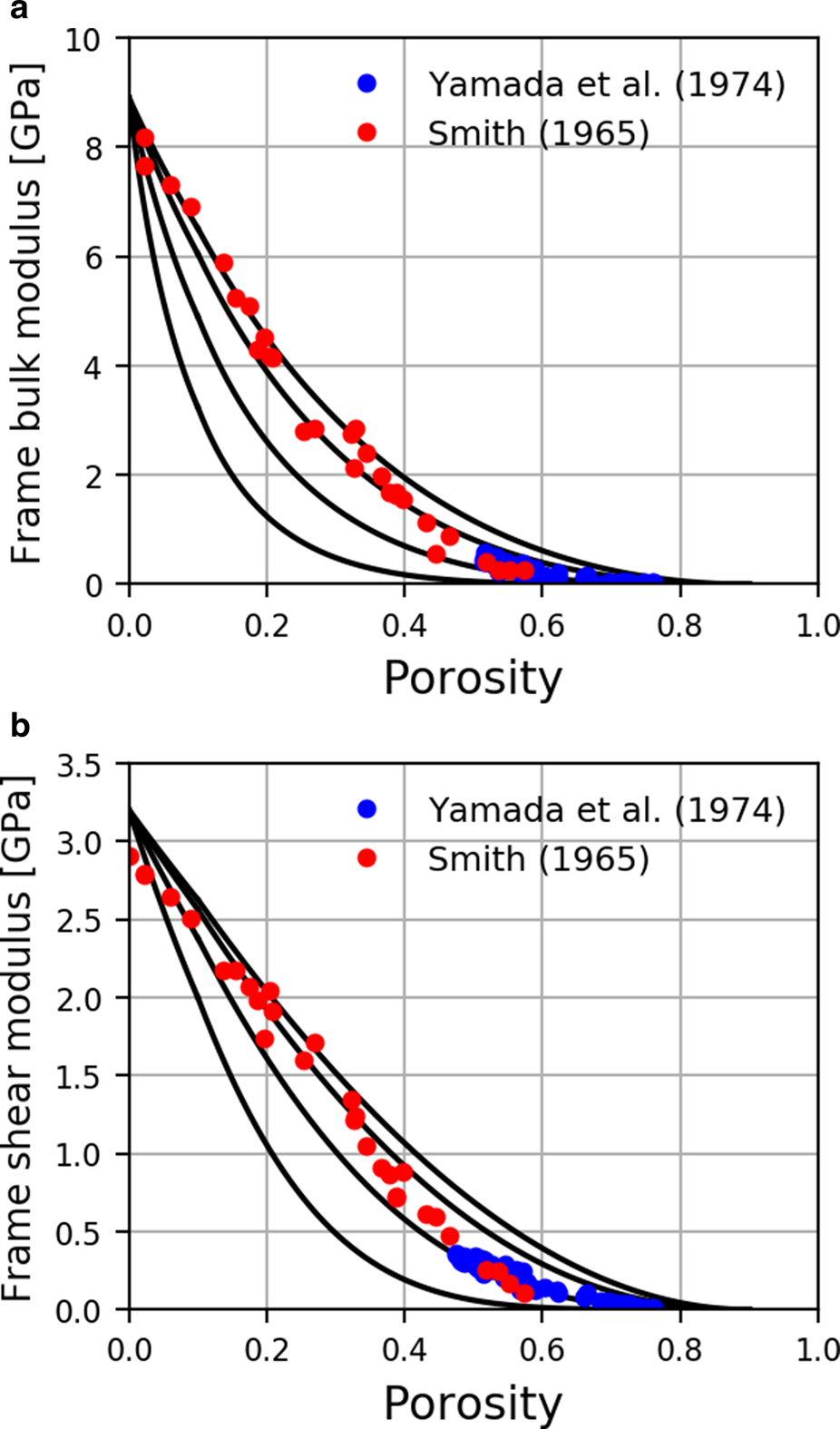
Fig. 5. (a) Bulk and (b) shear moduli (full curves) of the ice frame in dry snow and firn obtained using the modified differential effective medium scheme described in this paper assuming a critical porosity ϕc = 0.9 for inclusion aspect ratios of 0.1 (lower curve), 0.2, 0.4 and 1 (upper curve). The symbols show the measurements of Smith (Reference Smith1965) (red points) and Yamada and others (Reference Yamada, Hasemi, Izumi and Sata1974) (blue points).
Discussion
The previous section showed that the elastic moduli predicted using the modified differential effective medium scheme agree well with those deduced from the fast P- and S-velocity measurements of Smith (Reference Smith1965) and Yamada and others (Reference Yamada, Hasemi, Izumi and Sata1974). However, the shear modulus of ice in snow used is lower than values computed from the single crystal elastic stiffnesses of ice shown in Table I. This may indicate that the bond between ice particles is not perfect. To illustrate this, consider Figure 6, which shows a schematic representation of the interface between two ice particles in snow or firn. The bond between ice particles is treated as an imperfectly bonded interface across which the traction vector with Cartesian components t i, i = 1, 2, 3 is continuous but the displacement vector with Cartesian components u i may be discontinuous. Following Schoenberg (Reference Schoenberg1980) and Kachanov (Reference Kachanov1992) we assume that the discontinuity in displacement $[ u_i] \equiv {u_i^ + } - {u_i^-}$ between opposing faces of an interface is linear in the traction, so that

Here, B ij are components of the second-rank compliance tensor characterizing the mechanical properties of the interface, and the Einstein summation convention is adopted in which a sum over repeated indices is implied.

Fig. 6. Schematic representation of part of a bond between two ice particles in snow or firn modeled as a locally flat imperfectly bonded interface. The normal and shear displacements of the upper face of the interface are denoted by $u_N^ +$ and $u_S^ +$
 , whereas those of the lower face are denoted by $u_N^-$
 and $u_S^-$
 . The normal and shear tractions are denoted by t N and t S, respectively.
The contribution of the interfaces to the effective elastic properties may be written (Kachanov, Reference Kachanov1992; Sayers and Kachanov, Reference Sayers and Kachanov1995) in terms of a second- and fourth-rank tensor αij and βijkl defined by Kachanov (Reference Kachanov1992):


The terms $B_N^{( r) }$ and $B_S^{( r) }$
 are the effective normal and shear compliance of the rth interface in volume V, $n_i^{( r) }$
 is the ith component of the normal to the rth interface and A (r) is the area of the rth interface (Kachanov, Reference Kachanov1992; Sayers and Kachanov, Reference Sayers and Kachanov1995).
Assuming that snow and firn are isotropic, the non-vanishing components of αij and β ijkl are:


It then follows (Sayers and Han, Reference Sayers and Han2002; Sayers, Reference Sayers2018) that the bulk and shear moduli of the medium in the presence of imperfect bonds between the ice particles are:


where K 0 and μ 0 are the bulk and shear moduli that would result if the bonds between ice particles were perfect. It follows from Eqns (15) and (16) that 5β/(3α) = (B N/B S) − 1, assuming an isotropic distribution of normal vectors n i. Equations (20) and (21) then give:


It is seen that if B N/B S is small the bulk modulus K is relatively unaffected by the presence of imperfect bonding between ice particles, while the shear modulus μ is reduced significantly. Thus the reduced value of the shear modulus of ice required to obtain agreement with the shear modulus of snow and firn calculated from the P- and S-velocity measurements of Smith (Reference Smith1965) and Yamada and others (Reference Yamada, Hasemi, Izumi and Sata1974) in the preceding sections may indicate that the bonds between ice particles in snow and firn are more deformable under shear than under compression.
Although the reduced shear modulus μ s = 3.20 GPa used in the previous section gave good overall agreement with the measured elastic moduli shown in Figure 5, the shear modulus calculated from the measured S-wave velocities of Smith (Reference Smith1965) for low porosity are lower than this value. This may indicate that the c-axes of ice crystals in snow and firn investigated by Smith (Reference Smith1965) become partially aligned as porosity decreases. In support of this it is seen in Table I that the shear modulus C 55 corresponding both to S-wave propagation along the c-axis, and to S-wave propagation perpendicular to the c-axis with polarization along the c-axis, is significantly smaller than that given by the Hill average μ H. Since the elastic stiffness C 33 corresponding to P-wave propagation along the c-axis is significantly higher than the Hill average M H, while the elastic stiffness C 11 corresponding to P-wave propagation perpendicular to the c-axis is reasonably close to M H a comparison with Figures 4 and 5 suggests that the direction of propagation would need to be approximately perpendicular to the c-axes of the ice crystals for anisotropy to explain the reduced shear modulus at low porosity. Unfortunately, the direction of propagation is not given by Smith (Reference Smith1965), so that this hypothesis cannot be checked. Finally, it should be noted that the five lowest porosity samples (ρ > 800 kg m−3) studied by Smith (Reference Smith1965) were obtained by thermal drilling, while those with density (ρ < 800 kg m−3) were obtained using a 3-in diameter snow auger. If partial melting of the bonds between ice particles occurred during thermal drilling this might explain these low values of shear modulus following the discussion above. Alternatively, if thermal drilling led to the presence of liquid water in the pore space then the porosity calculated from density would be higher than shown in Figures 4 and 5 leading to the low porosity points in these figures being moved to higher porosity, as can be seen from Eqn (13).
Conclusion
Elastic wave velocity measurements provide a non-destructive method for estimating the mechanical properties, elastic wave velocities and density of snow and firn. Mechanical properties are needed for applications such as construction on snow, snow removal, vehicle mobility and avalanche release and control (Salm, Reference Salm1982). The elastic moduli of snow and firn are required for the interpretation of seismic measurements, which have been used to monitor and locate avalanches (Suriñach and others, Reference Suriñach, Vilajosana, Khazaradze, Biescas, Furdada and Vilaplana2005; Van Herwijnen and Schweizer, Reference Van Herwijnen and Schweizer2011; Lacroix and others, Reference Lacroix2012). Estimates of the variation of density with depth in snow deposited on glaciers and ice sheets enable improved monitoring of the surface mass balance of glaciers and ice sheets using airborne or satellite altimetry by allowing the measured surface elevation over time to be corrected for compaction of snow.
The elastic moduli of dry snow and firn are modeled using a modified differential effective medium scheme that accounts for the critical porosity above which the bulk and shear moduli of the frame vanish. The most complete datasets with measurements of density, fast P- and S-velocities are those of Smith (Reference Smith1965) and Yamada and others (Reference Yamada, Hasemi, Izumi and Sata1974). The expressions for the elastic properties of snow and firn as a function of porosity are compared, therefore, with these measurements. Comparison of the predicted bulk and shear moduli with those calculated from the P- and S-velocity measurements of Smith (Reference Smith1965) and Yamada and others (Reference Yamada, Hasemi, Izumi and Sata1974) shows that the modified differential effective medium scheme gives a good description of the data. This method is consistent with the expected zero moduli for porosity greater than a critical porosity ϕ c, assumed in this paper to take the value 0.9, and does not require an assumption of small pore aspect ratios at high porosity as needed with the original differential effective medium scheme. The results suggest that the shear modulus of ice in snow and firn is lower than that computed from single crystal elastic stiffnesses of ice. This may indicate that the bonds between snow particles are more deformable under shear than under compression. A partial alignment of ice crystals also may contribute.
It should be noted that the pore space in snow and firn is assumed, in this paper, to be air-filled, and no correction for the presence of melt water was performed since information on the presence or absence of melt water in the samples for which measurements were made was not available. Melting and refreezing would lead to a stiffening of the ice frame and an increase in the elastic moduli, and this would need to be corrected for if it occurs.
The model of elastic moduli of snow and firn as a function of porosity reported here is simple and compact, and does not require the use of empirical fits to the data. Owing to its simplicity, it is anticipated that this model may be useful in a variety of potential applications such as construction on snow, interpretation of seismic measurements to monitor and locate avalanches, and estimation of density within compacting snow deposited on glaciers and ice sheets.
Acknowledgements
I thank Achille Capelli for providing the data in Capelli (Reference Capelli2021), and the reviewers and Scientific Editor for many useful comments that lead to a significantly improved manuscript.
Appendix A.
Velocities in the high frequency limit of Biot theory
It is convenient to denote porosity by ϕ, density and bulk modulus of the solid (ice) by ρ s and K s, density and bulk modulus of the fluid (air) by ρ f and K f, and bulk and shear moduli of the ice frame by K b and μ b. In the high frequency limit, the P- and S-wave velocities are non-dispersive and are given by Johnson (Reference Johnson, Burridge, Childress and Papanicolaou1982a) as:


In these equations, τ > 1 is a geometrical quantity related to the tortuosity of the pore space in terms of which:


The quantities P, Q and R are given by:


The quantity Δ is defined by:


 Open access