
Abstract
Fuzzy analytic hierarchy process (FAHP) has been extensively applied to multi-criteria decision making (MCDM). However, the computational burden resulting from the calculation of fuzzy eigenvalue and eigenvector is heavy. As a result, a FAHP problem is usually solved using approximation techniques such as fuzzy geometric mean (FGM) and fuzzy extent analysis (FEA) instead of exact methods. Therefore, the FAHP results are subject to considerable inaccuracy. To solve this problem, in this study, a FAHP method based on the combination of α-cut operations (ACO), center-of-gravity (COG) defuzzification and defuzzification convergence mechanism (DCM) is proposed. First, ACO is applied to derive the near-exact fuzzy maximal eigenvalue and fuzzy weights. Subsequently, the α cuts of the fuzzy maximal eigenvalue and fuzzy weights are interpolated to generate samples that are uniformly distributed along the x-axis so that COG can be correctly applied to defuzzify the fuzzy maximal eigenvalue and fuzzy weights. To accelerate the computation process, DCM is applied to terminate the enumeration process if the defuzzified values of fuzzy weights have converged. The ACO–COG–DCM method has been applied to a real case to illustrate its applicability. In addition, a simulation study was also conducted to perform a parametric analysis. According to the experimental results, the proposed ACO–COG–DCM method improved the accuracy of estimating fuzzy weights by up to 56%. Furthermore, the experimental results also showed that the inaccuracy of estimating fuzzy weights was mostly owing to the deficiency of the FAHP method rather than the inconsistency of fuzzy pairwise comparison results.
1 Introduction
Fuzzy analytic hierarchy process (FAHP) was introduced by Van Laarhoven and Pedrycz (1983), and has been extensively applied to multi-criteria decision making (MCDM) problems in various fields, e.g., worker safety assessment (Zheng et al. 2012), supplier selection (Junior et al. 2014), text summarization (Güran et al. 2017), prioritizing the goals of waste elimination in lean manufacturing (Gnanavelbabu and Arunagiri 2018), identifying the critical barriers to reverse logistics (Sirisawat and Kiatcharoenpol 2018), cost-effect analysis (Donais et al. 2019), and others (Ljubojević et al. 2019; López et al. 2017; Schito et al. 2019).
Various methods have been proposed to solve a FAHP problem by deriving or approximating the eigenvalue and eigenvector of the fuzzy pairwise comparison matrix. For example, the fuzzy geometric mean (FGM) method proposed by Buckley (1985), the fuzzy extent analysis (FEA) method proposed by Chang (1996), the method based on α-cut operations (ACO) (Cheng and Mon 1994), the fuzzy prioritization method (FPM) (Wang et al. 2007), and others. The former three methods are more prevalent than the last method. Each method has its variants.
FGM and FEA are efficient, but approximate fuzzy weights instead of deriving them (Saaty 1996; Gu and Zhu 2006; Chen 2020; Wang and Chen 2019). Therefore, both methods are approximation methods. FGM and FEA are also subject to drawbacks such as inaccuracy, poor robustness, unreasonable priorities, information loss, and inflexibility (Kubler et al. 2016). Among them, inaccuracy means that weights do not reflect the real relative importance levels of attributes, criteria, or alternatives. In contrast, the ACO method derives the membership functions of fuzzy eigenvalue and vector. ACO is an exact method if a sufficient number of α values are considered. Therefore, ACO is accurate but is time-consuming. Due to the efficiency consideration, FGM and FEA have been more prevalent than ACO in practice. However, it is, in fact, not necessary to obtain the values of fuzzy weights within a very short period of time. In addition, advances in computer and computation technologies have considerably enhanced the efficiency of ACO. For these reasons, ACO is expected to gain more popularity in the future.
The inaccuracy of estimating fuzzy weights using approximation methods such as FGM and FEA has rarely been quantitatively analyzed in the past. However, this is a critical issue, since approximation methods are very prevalent in practice. Otherwise, overestimated or underestimated fuzzy weights may mislead the decision-making process. To address this issue and improve the accuracy of estimating fuzzy weights, in this study, a FAHP method based on the combination of ACO, center-of-gravity (COG) defuzzification and defuzzification convergence mechanism (DCM) is proposed. In the proposed methodology, first ACO is applied to derive the fuzzy maximal eigenvalue and fuzzy weights. The results are expected to be very close to their exact values. Subsequently, the fuzzy maximal eigenvalue and fuzzy weights are defuzzified using the prevalent COG method. However, ACO takes samples uniformly along the y-axis, while COG requires that samples be taken regularly along the x-axis. To address this inconsistency, the α cuts of the fuzzy maximal eigenvalue (or a fuzzy weight) are interpolated to generate samples that are uniformly distributed along the x-axis, so as to facilitate the application of COG. In addition, to accelerate the computation process, DCM is applied to terminate the enumeration process ACO if the defuzzified values of fuzzy weights have converged since in practical applications only the defuzzified values of fuzzy weights are concerned. In existing FAHP methods, the dependence between variables is usually ignored to accelerate the computation process.
The proposed ACO–COG–DCM method has been applied to a real case to illustrate its applicability. Some existing approximation methods were also applied to the real case to make a comparison. In addition, a simulation experiment was also conducted to perform a parametric analysis to gain some insights into the problems of existing FAHP methods. The differences between the proposed methodology and some existing FAHP methods are summarized in Table 1. The accuracy of ACO is not the highest because of the lack of a suitable defuzzifier, as stated above, which is tackled in the proposed methodology.
The remainder of this paper is organized as follows. Section 2 is devoted to the literature review. Section 3 provides some preliminaries. Section 4 details the proposed ACO–COG–DCM method. A real case is adopted to illustrate the applicability of the ACO–COG–DCM method in Sect. 5. In Sect. 6, a simulation experiment is conducted to perform a parametric analysis. Finally, Sect. 7 concludes this paper and provides some directions for future research.
2 Literature review
Although FAHP is computationally more complex than AHP, FAHP applications have been more and more popular due to advances in computer and computation technologies. The statistics on the number of FAHP related references by Google Scholar are presented in Fig. 1. FGM and FEA are the most prevalent techniques for solving a FAHP problem (Zheng et al. 2012; Sirisawat and Kiatcharoenpol 2018). FEA is especially welcomed because the weights of criteria are estimated in crisp values and do not need to be defuzzified further (Junior et al. 2014; Güran et al. 2017; Gnanavelbabu and Arunagiri 2018). However, the reasoning mechanism of FGM is more similar to the original reasoning mechanism of AHP than FEA. In addition, both techniques are based on approximation. The estimated fuzzy maximal eigenvalue and fuzzy weights are subject to imprecision.

(Data source: Google Scholar)
Statistics on the number of FAHP related references
In this section, some recent references on FAHP related applications are reviewed. For a customer lifetime value analysis, Pramono et al. (2019) applied FEA to determine the weights of four criteria—length, recency, frequency, and monetary value. Then, a simple weighted average was applied to assess the lifetime value of a customer. The application presented by Pramono et al. (2019) is very simple and typical for FAHP. Kaewfak et al. (2019) combined FEA and fuzzy technique for order of preference by similarity to ideal solution (TOPSIS) for selecting the optimal multimodal freight transportation routes. The weights of criteria determined using FEA became inputs to fuzzy TOPSIS. Although weights were estimated in crisp values, the performances of alternatives were assessed with triangular fuzzy numbers (TFNs), which explained why fuzzy TOPSIS, instead of TOPSIS, was adopted in their study. Lima-Junior and Carpinetti (2020) highlighted the problem of FEA—it was easy to get some weights with zero values. To solve this problem, five variants of FEA for solving this problem were compared. These variants either derived or defuzzified the synthetic extent of a criterion in different ways. Their conclusion was that the variant proposed by Ahmed and Kilic (2015) was the most effective in solving the problem without affecting the consistency of results. However, in our view, FEA is for approximation in nature, whether these extensions are necessary is debatable.
With higher computing power, whether decision-makers should still adhere to approximation methods, such as FEA and FGM, for convenience is questionable. To address this issue, an exact solution technique, such as ACO, is helpful. However, Zhü (2014) highlighted the problem of existing ACO applications (e.g., Promentilla et al. 2008)—only a few α cuts, rather than the membership function (i.e., all α cuts), of a fuzzy variable were considered. For solving this problem, a possible treatment is to enumerate as many α cuts as possible for each fuzzy variable, which obviously requires a time-consuming calculation process. For example, Chen (2020) proposed the FGM–ACO-fuzzy weighted average (FWA) method to evaluate the sustainability of a smart technology application to mobile health care, in which decision-makers’ judgments were aggregated using FGM before deriving the fuzzy weights of criteria using ACO. Subsequently, the derived fuzzy weights were fed as inputs to FWA to evaluate the sustainability of a smart technology application to mobile health care. The results obtained by the FGM–ACO–FWA method was more precise than those obtained by FGM or FEA. However, the required calculation process was time-consuming.
3 Preliminaries
3.1 Alpha cut and operations
First, the definition of an α cut is given.
Definition 1
(α cut). An α cut of a fuzzy set \(\tilde{F}\) is a crisp set \(F(\alpha )\) that contains all the elements of the universal set U which memberships in \(\tilde{F}\) are greater than or equal to α.
The α cut of a fuzzy number \(\tilde{A}\) can be expressed with the interval \(A(\alpha ) = [A^{L} (\alpha ),\;A^{R} (\alpha )]\). An arithmetic operation on two fuzzy numbers \(\tilde{A}\) and \(\tilde{B}\) can be performed based on their α cuts as follows:
-
(1)
Fuzzy addition:
$$(\tilde{A}( + )\tilde{B})(\alpha ) = [A^{L} (\alpha ) + B^{L} (\alpha ),\;A^{R} (\alpha ) + B^{R} (\alpha )]$$(1) -
(2)
Fuzzy subtraction:
$$(\tilde{A}( - )\tilde{B})(\alpha ) = [A^{L} (\alpha ) - B^{R} (\alpha ),\;A^{R} (\alpha ) - B^{L} (\alpha )]$$(2) -
(3)
Fuzzy multiplication:
$$(\tilde{A}( \times )\tilde{B})(\alpha ) = [A^{L} (\alpha )B^{L} (\alpha ),\;A^{R} (\alpha )B^{R} (\alpha )]\;{\text{if}}\;A^{L} (\alpha ),\;B^{L} (\alpha ) \ge 0$$(3) -
(4)
Fuzzy division:
$$(\tilde{A}(/)\tilde{B})(\alpha ) = [A^{L} (\alpha )/B^{R} (\alpha ),\;A^{R} (\alpha )/B^{L} (\alpha )]\;{\text{if}}\;A^{L} (\alpha ) \ge 0,\;B^{L} (\alpha ) > 0$$(4)
3.2 Some existing FAHP methods
FAHP is composed of the following steps (see Fig. 2):

The ACO result take samples more frequently from the left-hand side than from the right-hand side
-
(1)
Construct the fuzzy pairwise comparison matrix \({\tilde{\mathbf{A}}}\).
-
(2)
Derive or estimate the fuzzy eigenvalue and eigenvector of \({\tilde{\mathbf{A}}}\): Based on the results, the fuzzy maximal eigenvalue and fuzzy weights can be obtained.
-
(3)
Evaluate the consistency of fuzzy pairwise comparison results.
-
(4)
If fuzzy pairwise comparison results are not consistent, return to Step (1); otherwise, proceed to Step (5).
-
(5)
(Optional) Defuzzify and re-normalize fuzzy weights.
In FAHP, a fuzzy pairwise comparison matrix is constructed as:
where
\(\tilde{a}_{ij}\) is the fuzzy pairwise comparison result embodying the relative importance of criterion i over criterion j. 1 ≤ i, j ≤ n. Basically, \(0 < \tilde{a}_{ij} \le 9\). \(\tilde{a}_{ij}\) is a positive comparison if \(\tilde{a}_{ij} \ge 1\). The fuzzy eigenvalue and eigenvector of \({\tilde{\mathbf{A}}}\), indicated respectively with \(\tilde{\lambda }\) and \({\tilde{\mathbf{x}}}\), satisfy
and
The maximal fuzzy eigenvalue and the fuzzy weight of each criterion are derived respectively as
Based on \(\tilde{\lambda }_{\hbox{max} }\), the consistency of fuzzy pairwise comparison results is evaluated as
where R.I. is the random index (Satty 1980). As suggested by Satty (1980), a consistency index (or ratio) should be less than 0.1 for pairwise comparison results to be consistent. However, for a large or complicated problem, the threshold can be slightly relaxed, e.g., to 0.3 (Wedley 1993; Business Performance Management Singapore 2013). A fuzzy AHP problem is more complicated than a crisp AHP problem. Therefore, in the proposed methodology, fuzzy pairwise comparison results are considered inconsistent if \(\widetilde{{{\text{C}} . {\text{I}} .}} > 0.3\) or \(\widetilde{{{\text{C}} . {\text{R}} .}} > 0.3\).
3.3 FGM
The FGM method approximates the values of fuzzy weights as
Based on (13), the fuzzy eigenvalue can be estimated as
A variant of FGM (a simplified yet more prevalent version), indicated with FGMi, is to ignore the dependency between the dividend and divisor of either equation. Fuzzy weights approximated using FGM or FGMi can be defuzzified to generate crisp weights, after which a re-normalization step may be required.
3.4 FEA
The FEA method starts by evaluating the fuzzy synthetic extent of each criterion as:
Then, the weight of the criterion is set to its minimal degree of being the maximum (MDBM):
where
In this way, the obtained weight is crisp and, therefore, does not need additional defuzzification and renormalization. However, it is difficult to infer the value of \(\tilde{\lambda }_{\hbox{max} }\) from \(\{ w_{j} \}\). Ignoring the dependency between the dividend and divisor of Eq. (15) results in a simplified version indicated with FEAi.
3.5 ACO
Replacing the fuzzy parameters and variables in Eqs. (7) and (8) with their α cuts leads to
where each α cut is an interval:
Then,
If α takes 11 possible values (0, 0.1, …, 1), Eqs. (18) and (19) need to be solved 11 · \(2^{{\text{C}_{2}^{n} }}\) times to derive the membership functions of fuzzy eigenvalue and eigenvectors. In the past studies like Csutora and Buckley (2001), only the results when α = 0 or 1 were derived owing to the inefficiency problem.
A simplified version, indicated with ACOw, is to consider the weighted mean of α cuts instead of their individual values (Promentilla et al. 2008):
In this way, the FAHP problem becomes a crisp AHP problem for each α value.
4 The proposed methodology
The proposed methodology involves three stages. The first stage is to apply ACO to derive the fuzzy maximal eigenvalue and fuzzy weights according to Eqs. (18)–(23). Because many fuzzy multiplication operations are involved, the shapes of the membership functions of the fuzzy maximal eigenvalue and fuzzy weights are not the same with those of \(\tilde{a}_{ij}\)’s.
Crisp weights are usually required in practice. Therefore, the second stage of the proposed methodology is to defuzzify the fuzzy maximal eigenvalue and fuzzy weights using COG. In ACO, the y-axis (representing the α value) is partitioned into equal intervals, as illustrated in Fig. 2. However, COG is based on the integral with respect to the variable on the x-axis (i.e., either \(\tilde{\lambda }_{\hbox{max} }\) or \(\tilde{w}_{i}\)). Therefore, COG cannot be directly applied to defuzzify the ACO results. For example, if the membership function \(\tilde{w}_{i}\) is skewed to the right, as in Fig. 2, the ACO results will take samples more frequently from the left-hand side than from the right-hand side. As a result, the COG result under-estimates \(\tilde{w}_{i}\). In Fig. 2, the defuzzified value of \(\tilde{w}_{i}\) using COG should be 0.0365, while that based on the ACO results is only 0.0329. The deviation is up to 10%. Conversely, if the membership function is skewed to the left, then the defuzzification result will be over-estimated.
Taking \(\tilde{w}_{i}\) as an example, the α cuts are interpolated to generate samples that are uniformly distributed along the x-axis in the following manner:
In Eq. (25), the x-axis is partitioned into K equal intervals (see Fig. 3). In Eq. (26), the membership of \(w_{j}^{t} (k)\) is estimated by the interpolation of the two nearest α cuts, as shown in Fig. 4. Based on the results, \(\tilde{w}_{j}\) is defuzzified using COG as

Partitioning the x-axis into K equal intervals

Interpolation of the two nearest α cuts
After defuzzification, crisp weights may not sum up to 1 and need to be re-normalized.
When only the defuzzified values of the fuzzy maximal eigenvalue and fuzzy weights are concerned, the ranges of these fuzzy variables become unimportant, which lessens the necessity to enumerate all possible combinations. In addition, with limited results (i.e., k ≪ 11 · \(2^{{\text{C}_{2}^{n} }}\)), the defuzzification formula (27) is still applicable, and the defuzzification result is expected to converge gradually as K increases. Such a mechanism is called DCM in the third stage:
-
Step 1. Set k = 1.
-
Step 2. Choose the k-th combination.
-
Step 3. Derive the maximal eigenvalue and weights.
-
Step 4. Defuzzify the fuzzy maximal eigenvalue and fuzzy weights using Eqs. (21)–(23).
-
Step 5. If the defuzzification results converge, go to Step 8; otherwise, go to Step 6: Two stopping criteria for judging the convergence of the defuzzification results are
-
(i)
Maximal absolute deviation from the previous value < 0.001;
-
(ii)
Maximal absolute deviation percentage from the previous value < 0.5%.
-
(i)
-
Step 6. k = k + 1.
-
Step 7. If k = 11 · \(2^{{\text{C}_{2}^{n} }}\), go to Step 8; otherwise, go to Step 2.
-
Step 8. Stop.
5 An illustrative case
The supplier selection problem discussed by Junior et al. (2014) is taken as an example to illustrate the application of the proposed ACO–COG–DCM approach. In this case, each supplier had five attributes (i.e., quality, price, delivery, supplier profile, and supplier relationship) that were considered critical to choosing a suitable supplier. TFNs were adopted to express fuzzy variables and parameters. After a series of pairwise comparisons, the following fuzzy pairwise comparison matrix was constructed:
The ACO–COG–DCM approach was applied to derive the fuzzy maximal eigenvalue and the fuzzy weights of the five attributes. Eleven possible values of α, from 0, 0.1, …, to 1, were considered. As a result, the eigenvalue and eigenvector of the fuzzy pairwise comparison matrix needed to be solved 10 · \(2^{{\text{C}_{2}^{5} }}\) + 1 = 10,241 times. MATLAB 2017 was adopted to implement the ACO–COG–DCM approach on a PC with i7-7700 CPU 3.6 GHz and 8 GB RAM. The execution time was about 12 s. Finally, the derived fuzzy maximal eigenvalue and fuzzy weights are shown in Figs. 5 and 6, respectively. Although \(\tilde{a}_{ij}\)’s were given in TFNs, the fuzzy maximal eigenvalue and fuzzy weights were considerably different from TFNs.

The fuzzy maximal eigenvalue

Fuzzy weights
The α cuts of the fuzzy maximal eigenvalue and fuzzy weights were interpolated to generate samples that are uniformly distributed along the x-axis. Then, COG was applied to defuzzify fuzzy variables. The results are summarized in Table 2. For a comparison, the traditional way, i.e., defuzzifying fuzzy variables based on their α cuts directly, was also applied. The results are presented in the same table. Among fuzzy variables, the membership functions of \(\tilde{\lambda }_{\hbox{max} }\), \(\tilde{w}_{1}\), \(\tilde{w}_{3}\), \(\tilde{w}_{4}\), and \(\tilde{w}_{5}\) were skewed to the right. As a consequence, defuzzifying these fuzzy variables based on their α cuts directly under-estimated the results. Conversely, the membership function of \(\tilde{w}_{2}\) was skewed to the left, causing it being over-estimated.
After defuzzification, the sum of crisp weights was not equal to 1. So, crisp weights were re-normalized. The results are shown in Table 3.
To further elaborate on the effectiveness of the proposed methodology, five existing FAHP methods were also applied to this case. In the ACOw method, η was set to 0.5. The results are summarized in Figs. 7 and 8.

The values of \(\tilde{\lambda }_{\hbox{max} }\) obtained by existing methods


The values of fuzzy weights obtained by existing methods
From the results, the following discussion was made:
-
(1)
The values of the fuzzy maximal eigenvalue (\(\tilde{\lambda }_{\hbox{max} }\)) estimated using FGM, FGMi, FEA and FEAi were still TFNs, while that obtained by ACOw was not.
-
(2)
The values of fuzzy weights estimated using FGM and FGMi were still TFNs, while those obtained by ACOw were not. The values of weights estimated using FEA and FEAi were crisp.
-
(3)
The cores (i.e., values with a membership of 1) of the fuzzy maximal eigenvalue obtained by FGM, FGMi and ACOw were quite close to each other but were considerably different from those obtained by FEA and FEAi. As mentioned previously, the MDBM function applied in FEA and FEAi made it difficult to infer the fuzzy maximal eigenvalue from fuzzy weights.
-
(4)
The ranges of \(\tilde{\lambda }_{\hbox{max} }\) estimated using FGM and FGMi were much (17 to 27 times) wider than that estimated using the ACO–COG–DCM method. The range estimated using ACOi could not cover all possible values of \(\tilde{\lambda }_{\hbox{max} }\) because of the loss of information (about the ranges of fuzzy pairwise comparison results). The ranges estimated using FEA and FEAi were not reliable because of the reason mentioned in (3).
-
(5)
The fuzzy consistency index and fuzzy consistency ratio were evaluated to check whether pairwise comparison results were consistent or not. The results are summarized in Table 4. Two methods, middle of maxima (MOM) and center of gravity (COG), were both applied to defuzzify them to make a judgment. MOM was also applied because the defuzzification results were the consistency index and consistency ratio of the crisp AHP problem. A result of consistency is marked with an asterisk. Basically, fuzzy pairwise comparison results were consistent.
Table 4 Defuzzified value of \(\tilde{\lambda }_{\hbox{max} }\) -
(6)
Subsequently, the DCM mechanism was applied to enhance the computation efficiency by estimating the defuzzified values of fuzzy weights during the enumeration process. The changes in the defuzzified values of fuzzy weights during the enumeration process are shown in Fig. 9. In this case, the defuzzified values of fuzzy weights converged after enumerating only 54 combinations, less than 0.5% of the required combinations (i.e., 10,241 combinations). The estimated defuzzified values were compared with exact values (i.e., the defuzzified values after enumerating all combinations) in Table 5. Obviously, the defuzzified values estimated using the DCM mechanism were very accurate, even more accurate than those obtained by COG that enumerated all combinations without resampling, which was confirmed using the following paired sample t test:
Fig. 9 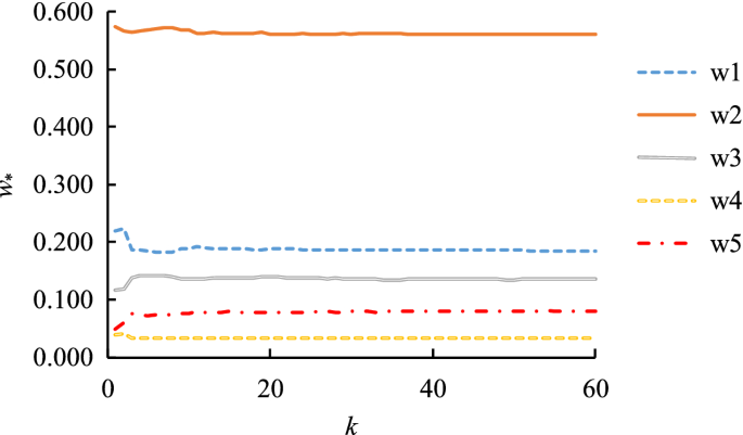
The changes of the defuzzified values of fuzzy weights during the enumeration process
Table 5 Estimating the defuzzified values of fuzzy weights using the DCM mechanism (k = 54)

H0
For improving the accuracy (in terms of the average absolute deviation from exact value) in estimating the defuzzified values of fuzzy weights, the performance of the DCM mechanism is the same as that of COG that enumerated all combinations without resampling.
H1
For improving the accuracy in estimating the defuzzified values of fuzzy weights, the performance of the DCM mechanism is better than that of COG that enumerated all combinations without resampling.
Table 6 presents a summary of the results. The null hypothesis H0 was rejected at a significance level of 0.1, indicating that the DCM mechanism was statistically superior to COG that enumerated all combinations without resampling in estimating the defuzzified values of fuzzy weights.
6 Further analyses
To carry out further analysis, a simulation experiment has been performed using MATLAB on the same PC. In the simulation experiment, five factors affected the goal, i.e., n = 5. A 5 × 5 fuzzy judgment matrix was considered because fuzzy judgment matrixes used in most past studies were smaller. In addition, a fuzzy judgment matrix had countless possible values regardless of its size, especially when multiple decision—makers were involved. For this reason, fuzzy judgment matrixes of various sizes were not tried in this study. The average time required to execute each method once for a 5 × 5 fuzzy judgment matrix is presented in Table 7.
The fuzzy pairwise comparison matrix was randomly generated. Nevertheless,
-
(1)
The reciprocal property was satisfied.
-
(2)
The consistency of fuzzy pairwise comparison results was ensured by requesting COG(\(\tilde{\lambda }_{\hbox{max} }\)) ≤ 0.2.
The simulation experiment was repeated 20 times. Fuzzy weights obtained by the three methods were defuzzified using COG and compared. The results are shown in Fig. 10.


Weights obtained by the three methods
According to the simulation results,
-
(1)
Obviously, the defuzzified values of fuzzy weights obtained using the two approximation methods (FGMi and FEAi) were different from those obtained using the exact method ACO.
-
(2)
Decision making based on the results obtained by approximation methods might be incorrect. In the experiment, it was assumed that there were six alternatives which performances were randomly generated and are shown in Table 8. The overall performance of each alternative was derived using the weighted average. Then, the top—performing alternative was chosen. The choices made by applying the three methods are summarized in Table 9, in which an incorrect choice was indicated with an asterisk. In total, the applications of FGMi and FEAi resulted in 3 and 6 incorrect choices, respectively, because the estimated fuzzy weights deviated from exact values.
Table 8 Performances of six alternatives Table 9 Choices made by applying various methods -
(3)
Therefore, the recommendation of this study is to apply ACO whenever possible. However, after experimentation, deriving fuzzy weights from a 6 * 6 fuzzy judgment matrix using ACO on an ordinary PC might take more than 10 min. As a result, FAHP problems with a smaller fuzzy judgment matrix can be easily solved using ACO.
-
(4)
Obviously, fuzzy weights estimated using FEAi deviated more, from exact values, than those estimated using FGMi did, meaning that FEAi was less accurate than FGMi. The mean absolute deviations (MADs) achieved using FGMi and FEAi were 0.018 and 0.058, respectively. The mean absolute percentage deviations (MAPDs) achieved using the two methods were 13% and 56%, respectively. To further examine this, the following paired sample t test was performed:
H0
In estimating the defuzzified values of fuzzy weights, the accuracy (in terms of the average absolute deviation from exact value) of FGMi is the same as that of FEAi.
H1
In estimating the defuzzified values of fuzzy weights, the accuracy of FGMi is better than that of FEAi.
The results are summarized in Table 10. The null hypothesis H0 was rejected at a significance level of 0.05, showing that FGMi outperformed FEAi in estimating the defuzzified values of fuzzy weights.
-
(5)
In either method, the absolute deviation (AD) of a weight was not closely related to its value, as shown in Fig. 11. This result implied that MAD could be used to estimate the deviation of a weight regardless of its value in both methods. However, the coefficient of determination (R2) was low.
Fig. 11 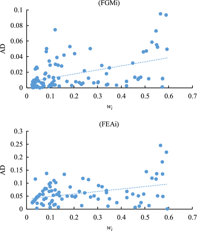
The AD of a weight versus its value
-
(6)
As a consequence, the absolute percentage deviation (APD) of a weight reduced with the increase in its value, as shown in Fig. 12, since APD was calculated by dividing AD by the value.
Fig. 12 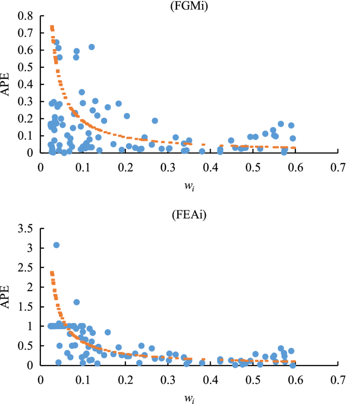
The APE of a weight versus its value
-
(7)
In addition, there was no clear relationship between C.R. and MAD, or between C.R. and MAPD, as shown in Fig. 13. Such a result revealed that an incorrect estimation of the values of fuzzy weights was mostly owing to the deficiency of the FAHP method rather than the inconsistency of the fuzzy pairwise comparison matrix.
Fig. 13 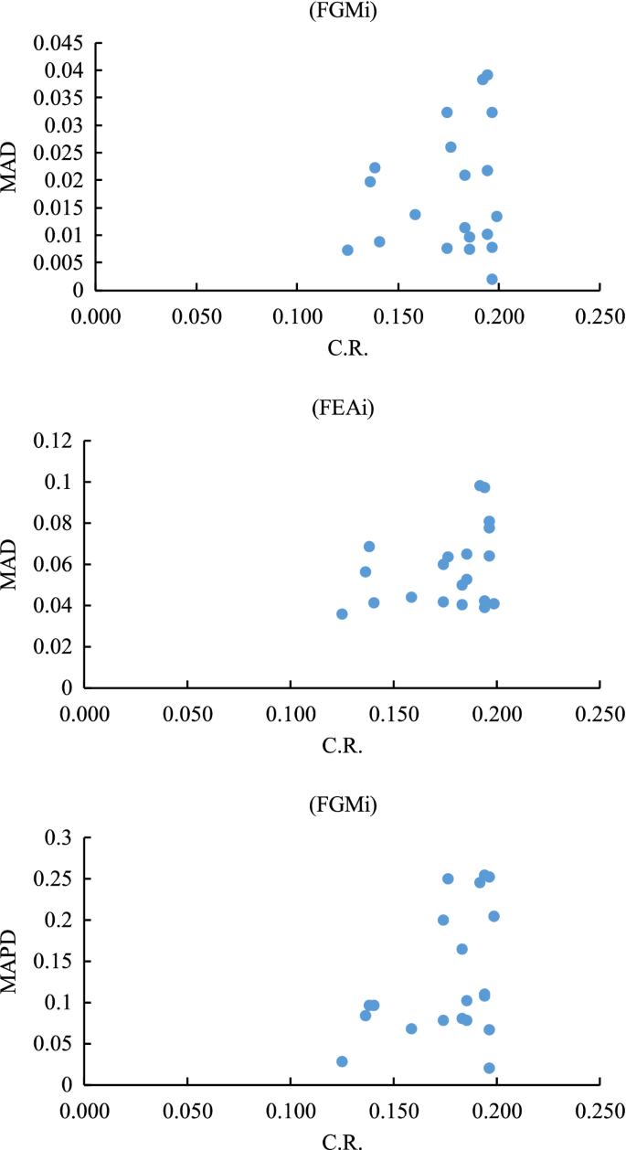
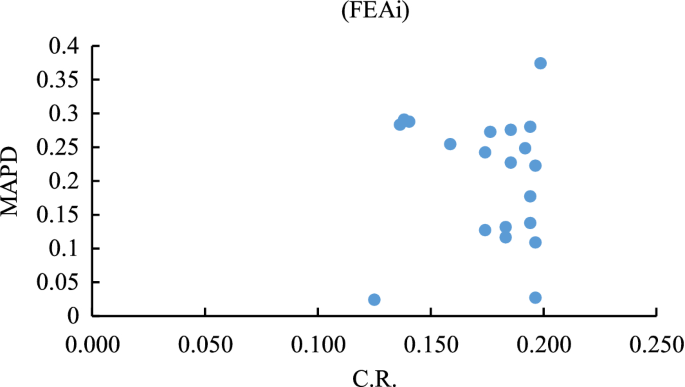
The relationship between C.R. and MAD (or MAPD)


7 Conclusions
FAHP has been extensively applied to determining the weights of criteria in a MCDM problem. However, prevalent FAHP methods, such as FGM and FEA, are subject to inaccuracy. To solve this problem, the ACO–COG–DCM approach is proposed in this study. In the proposed methodology, ACO is first applied to derive the fuzzy maximal eigenvalue and fuzzy weights. The results are very close to their exact values. Subsequently, to defuzzify the fuzzy maximal eigenvalue and fuzzy weights using COG accurately, their α cuts are interpolated to generate samples that are uniformly distributed along the x-axis. Finally, DCM is applied to accelerate the computation process. The ACO–COG–DCM approach has been applied to a real case to illustrate its applicability. In addition, a simulation experiment was also conducted for performing a parametric analysis.
According to the experimental results,
-
(1)
If the membership function of a fuzzy weight was skewed to the right, applying COG to defuzzify the ACO result directly under-estimated the weight. Conversely, if the membership function was skewed to the left, then the defuzzification result would be over-estimated.
-
(2)
FEAi was less accurate than FGMi.
-
(3)
On average, a fuzzy weight estimated using FGMi deviated from the exact value by 0.018. If FEAi was applied, the average deviation was up to 0.058. In addition, this deviation seemed to be independent of the value of the fuzzy weight.
-
(4)
Compared to the ineffectiveness of the FAHP method, the inconsistency of fuzzy pairwise comparison results was less influential to the accuracy of estimating the values of fuzzy weights.
More case studies can be conducted in future studies to validate the conclusions drawn in this study.
References
Ahmed F, Kilic K (2015) Modification to fuzzy extent analysis and its performance analysis. In: 6th international conference on industrial engineering and systems management (IESM), Seville, Spain
Buckley JJ (1985) Fuzzy hierarchical analysis. Fuzzy Sets Syst 17(3):233–247
Business Performance Management Singapore (2013) AHP—high consistency ratio. https://bpmsg.com/ahp-high-consistency-ratio/
Chang DY (1996) Applications of the extent analysis method on fuzzy AHP. Eur J Oper Res 95(3):649–655
Chen TCT (2020) Guaranteed-consensus posterior-aggregation fuzzy analytic hierarchy process method. Neural Comput Appl 32:7057–7068
Cheng CH, Mon DL (1994) Evaluating weapon system by analytical hierarchy process based on fuzzy scales. Fuzzy Sets Syst 63(1):1–10
Csutora R, Buckley JJ (2001) Fuzzy hierarchical analysis: the Lambda-Max method. Fuzzy Sets Syst 120(2):181–195
Donais FM, Abi-Zeid I, Waygood EOD, Lavoie R (2019) A review of cost–benefit analysis and multicriteria decision analysis from the perspective of sustainable transport in project evaluation. EURO J Decis Process 7(3):327–358
Gnanavelbabu A, Arunagiri P (2018) Ranking of MUDA using AHP and Fuzzy AHP algorithm. Mater Today Proc 5(5–2):13406–13412
Gu X, Zhu Q (2006) Fuzzy multi-attribute decision-making method based on eigenvector of fuzzy attribute evaluation space. Decis Support Syst 41(2):400–410
Güran A, Uysal M, Ekinci Y, Güran CB (2017) An additive FAHP based sentence score function for text summarization. Inf Technol Control 46(1):53–69
Junior FRL, Osiro L, Carpinetti LCR (2014) A comparison between Fuzzy AHP and Fuzzy TOPSIS methods to supplier selection. Appl Soft Comput 21:194–209
Kaewfak K, Huynh VN, Ammarapala V, Charoensiriwath C (2019) A fuzzy AHP-TOPSIS approach for selecting the multimodal freight transportation routes. In: International symposium on knowledge and systems sciences. Springer, Singapore, pp 28–46
Kubler S, Robert J, Derigent W, Voisin A, Le Traon Y (2016) A state-of the-art survey & testbed of fuzzy AHP (FAHP) applications. Expert Syst Appl 65:398–422
Lima-Junior FR, Carpinetti LCR (2020) Dealing with the problem of null weights and scores in Fuzzy Analytic Hierarchy Process. Soft Comput 24:9557–9573
Ljubojević S, Pamučar D, Jovanović D, Vešović V (2019) Outsourcing transport service: a fuzzy multi-criteria methodology for provider selection based on comparison of the real and ideal parameters of providers. Oper Res 19:399–433
López JCL, Carrillo PAÁ, Chavira DAG, Noriega JJS (2017) A web-based group decision support system for multicriteria ranking problems. Oper Res Int J 17(2):499–534
Pramono PP, Surjandari I, Laoh E (2019) Estimating customer segmentation based on customer lifetime value using two-stage clustering method. In: 2019 16th international conference on service systems and service management, pp 1–5
Promentilla MAB, Furuichi T, Ishii K, Tanikawa N (2008) A fuzzy analytic network process for multi-criteria evaluation of contaminated site remedial countermeasures. J Environ Manage 88(3):479–495
Saaty TL (1996) Decision making with dependence and feedback: the analytic network process. RWS Publications, Pittsburgh
Satty TL (1980) The analytic hierarchy process. McGraw-Hill, New York
Schito J, Jullier J, Raubal M (2019) A framework for integrating stakeholder preferences when deciding on power transmission line corridors. EURO J Decis Process 7(3–4):159–195
Sirisawat P, Kiatcharoenpol T (2018) Fuzzy AHP-TOPSIS approaches to prioritizing solutions for reverse logistics barriers. Comput Ind Eng 117:303–318
Van Laarhoven PJM, Pedrycz W (1983) A fuzzy extension of Saaty’s priority theory. Fuzzy Sets Syst 11(1–3):229–241
Wang YC, Chen TCT (2019) A partial-consensus posterior-aggregation FAHP method—supplier selection problem as an example. Mathematics 7(2):179
Wang L, Chu J, Wu J (2007) Selection of optimum maintenance strategies based on a fuzzy analytic hierarchy process. Int J Prod Econ 107(1):151–163
Wedley WC (1993) Consistency prediction for incomplete AHP matrices. Math Comput Model 17(4–5):151–161
Zheng G, Zhu N, Tian Z, Chen Y, Sun B (2012) Application of a trapezoidal fuzzy AHP method for work safety evaluation and early warning rating of hot and humid environments. Saf Sci 50(2):228–239
Zhü K (2014) Fuzzy analytic hierarchy process: fallacy of the popular methods. Eur J Oper Res 236(1):209–217
Acknowledgements
The author would like to thank the valuable comments of the editor and reviewers for improving the quality of this paper.
Author information
Authors and Affiliations
Corresponding author
Additional information
Publisher's Note
Springer Nature remains neutral with regard to jurisdictional claims in published maps and institutional affiliations.
Rights and permissions
About this article

Cite this article
Chen, T. Enhancing the efficiency and accuracy of existing FAHP decision-making methods. EURO J Decis Process 8, 177–204 (2020). https://doi.org/10.1007/s40070-020-00115-8
Received:
Accepted:
Published:
Issue Date:
DOI: https://doi.org/10.1007/s40070-020-00115-8
Keywords
- Fuzzy analytic hierarchy process
- Fuzzy geometric mean
- Fuzzy extent analysis
- Alpha-cut operations
- Accuracy
- Center-of-gravity