


Introduction
Since the rediscovery of dielectric waveguides (DWGs) as a medium for high data rate transmission at millimeter-wave (mm-wave) frequencies in 2010 [Reference Fukuda, Hino, Ohashi, Takeda, Yamagishi, Shinke, Komori, Uno, Akiyama, Kawasaki and Hajimiri1], a tremendous development has been observed in this field [Reference De Wit, Ooms, Philippe, Zhang and Reynaert2, Reference Holloway, Dogiamis and Han3]. From the beginnings until today, the achievable data rate over 1 m DWG has been tripled from 12 to 36 Gb/s [Reference Sawaby, Dolatsha, Grave, Chen and Arbabian4]. At the same time, the maximum transmission distance increased from 1 to 15 m [Reference Van Thienen, Zhang, De Wit and Reynaert5]. In order to further increase the data rate, the required components are constantly improved. Besides the optimization of transmitter and receiver units [Reference Sawaby, Dolatsha, Grave, Chen and Arbabian4, Reference Thienen, Zhang and Reynaert6], the increase in data capacity of DWG systems has been mainly achieved by improving the signal-to-noise ratio (SNR) at the receiver. The use of low-loss materials or different designs (e.g. hollow core fibers) for DWGs [Reference Kim, Nan, Cong and Chang7–Reference Van Thienen, Volkaerts and Reynaert9] as well as the enhanced coupling into DWGs [Reference Yu, Liu, Ye, Ren, Liu and Gu10–Reference Meyer and Schneider14] ensure a low insertion loss of the transmission channel and therefore increase the SNR at the receiver. In addition to signal distortions caused by noise, a broadband signal transmitted along a DWG is also disturbed by the frequency-dependent propagation characteristics of the DWG channel. These propagation characteristics include frequency-dependent attenuation and frequency-dependent group delay (waveguide dispersion) that can lead to intersymbol interference (ISI) in digital data transmission systems. The possibility to further improve the channel capacity by reducing frequency-dependent attenuation and frequency-dependent group delay of the DWG itself has not yet been completely investigated.
In [Reference Dolatsha, Chen and Arbabian15], the channel capacity of DWGs is approximated exemplarily for some solid and hollow core DWGs in the D-Band frequency range ($110 {-}170\, {\rm GHz}$ ) based on the frequency-dependent group delay. This rough first-order approximation indicates a $ {1}/{\sqrt {l}}$
 relation between maximum data rate and length l of the DWG. The authors concluded that waveguide dispersion is the limiting factor in a DWG data transmission system, and not insertion loss. A similar conclusion has been drawn in [Reference De Wit, Zhang and Reynaert16] where the dispersion caused by frequency-dependent group delay was identified as the main limitation of the presented data transmission. However, the authors also pointed out that frequency-dependent attenuation is not negligible. In both publications, the question remains unanswered how large the effect of frequency-dependent attenuation and group delay actually is and which DWGs lead to minimal signal distortions. Although Meyer et al. [Reference Meyer, Krüger and Schneider17] have shown that waveguide dispersion caused by frequency-dependent group delay in circular solid and hollow core DWGs can be minimized by appropriate design, it is still unclear how such a reduction would affect a transmission system in detail. Therefore, it is unknown to what extent DWGs have to be optimized to ensure negligible signal distortions. Furthermore, signal distortions caused by the frequency-dependent attenuation of the DWG, as well as its minimization, has not yet been investigated.
For this reason, this paper presents a detailed analysis of expected signal distortions that occur when data are transmitted via circular DWGs in the mm-wave frequency range. First, the data transmission system is described and the definitions of SNR and ISI for this system are introduced. Both SNR and ISI are used later to quantify the signal distortions. Subsequently, the frequency-dependent attenuation and frequency-dependent phase constant of DWGs are modeled by a Taylor series. In order to describe the frequency dependency of both values for common circular DWGs at mm-wave frequencies, a generalized analysis is given. The mathematical modeling for this analysis is specified on the basis of only two parameters, i.e. normalized frequency and normalized material properties. The general mathematical description allows the reader to directly calculate transmission properties, such as attenuation, group delay, and waveguide dispersion, of a wide range of circular DWGs that are typically used at mm-wave frequencies without the need of time consuming finite element method (FEM) simulations. Moreover, the given figures and equations can be used to calculate the expected signal distortions in a circular DWG. To determine the main cause of distortions in DWG systems, the effects of frequency-dependent attenuation and frequency-dependent group delay are analyzed separately. Finally, the combined effect of frequency-dependent attenuation and dispersion is considered, and recommendations for a DWG design are given to minimize signal distortions.
Data transmission system
To determine signal distortions along a DWG a low-complexity digital data transmission system as shown in Fig. 1 is assumed. In this communication system a data source generates an infinite pulse sequence

where d(i) represents the actual data to be transmitted. For example, d(i) can be a sequence of discrete voltage values of a sampled analog signal or output values of a digital data processing system. These data points are weighted by a Dirac impulse δ 0. The time between each impulse is the sampling period T. Since the impulse sequence (1) would have an infinite bandwidth, an ideal low-pass filter

is used as pulse shaping filter to limit the signal bandwidth of the transmitted signal to 2ωN. The cut-off frequency ωN of the filter fulfills the Nyquist–Shannon sampling theorem f N = ωN/2π = 1/2T. After the pulse shaping filter, the band-limited signal is transmitted via DWG. Additionally, the signal is superimposed by white Gaussian distributed noise n(t). To fulfill the matched filter criterion, the distorted signal is filtered at the receiver by an ideal low-pass filter (receive filter) given by (2). The filtered receive signal r(t) is then sampled with the sampling period T. This results in a disturbed signal sequence at the receiver, where each received symbol r(iT) can be described by

where iT represents the i-th sample point for a sampling period of T = π/ωN. The pulse shaping filter, the DWG as well as the receive filter are summarized as the channel impulse response h(t). It can be seen that the received symbol at time iT is not only the transmitted symbol d(i) disturbed by the channel impulse response (hereinafter called r 0(iT)), it is also superimposed by the time-shifted channel responses of all symbols d(k) that were transmitted before and after the actual symbol d(i) (hereinafter called Δr(iT)). This effect is well known as ISI.

Fig. 1. Schematic representation of a low-complexity digital data transmission system using a DWG as a channel.
In order to evaluate the signal distortions by the channel, the SNR and the ISI of the received symbols r(iT) are determined. For uncorrelated random data d(i) the SNR can be expressed by

where $\sigma _D^2$ and $\sigma _N^2$
 are the variances of the transmitted data sequence d(i) and noise n(iT). The ISI can be quantified by

Equations (4) and (5) depend solely on the impulse response h(t) of the transmission channel including filters and DWG. Since the filter characteristics are already described by (2), a mathematical description of the DWG channel is needed to calculate the signal distortions caused by the DWG. Due to the large variety of possible diameters and materials for circular DWGs in the mm-wave frequency band, a general description of the transmission behavior of circular DWGs is presented in Section “DWG channel.” Based on this description, the channel impulse response h(t) is derived in Section “Signal distortions” and the resulting signal distortions are determined using SNR and ISI.
DWG channel
The frequency response of a DWG in the bandpass domain can be described by

where γ(ω) is the frequency-dependent propagation constant

l the length of the waveguide and j the imaginary unit. The attenuation per unit length of an electromagnetic wave propagating along the DWG is characterized by the attenuation constant α whereas the phase change per unit length is described by the phase constant β. In practice, both constants are frequency-dependent. These frequency dependencies cause signal distortions while transmitting data along such a waveguide. To describe the frequency dependency mathematically, in this paper, real and imaginary parts of the propagation constant are approximated by a Taylor series. The Taylor series is calculated at the center frequency ω0 of the transmitted signal:

and

For the attenuation constant α, the Taylor coefficients are

The coefficient α0 corresponds to the attenuation per unit length at the center frequency ω0. The coefficient α1 represents the first-order frequency dependency of the attenuation in the frequency range around the center frequency ω0. For the phase constant β, the Taylor coefficients are

where β0 corresponds to the phase per unit length, β1 characterizes the group delay τg(ω0) per unit length, and β2 is a measure for the waveguide dispersion at the center frequency. The approximation of the attenuation constant and the phase constant using a Taylor series of first and second order has been found to be highly accurate for relative bandwidths up to $5$ –10%. For most DWGs, a larger relative bandwidth (up to $\approx \!30\percnt$
 ) would result in a frequency dependency of α(ω) and β(ω) that is slightly higher than the frequency dependency calculated by the Taylor approximation in this paper.
The transmission behavior of a DWG and consequently its propagation constant γ(ω) depends on the geometry and materials used as well as the operating frequency. In case of circular DWGs, the diameter D of the core in relation to the free-space wavelength λ0 significantly influences the transmission behavior. To illustrate this effect, the electric field E of the fundamental mode HE11 in a circular DWG is shown for different wavelengths related to its diameter in Fig. 2. The figure shows the cross section of a circular DWG consisting of a core with a diameter D and a relative permittivity ɛr,1 surrounded by a cladding with the relative permittivity ɛr,2. At low frequencies, meaning large wavelengths in relation to the DWG diameter (D/λ0 ≪ 1), the field of the fundamental mode HE11 spreads widely into the cladding material. With increasing frequency, the field is further concentrated within the core of the DWG until the mode propagates almost completely in the core (D/λ0 ≫ 1). In the mm-wave frequency range, DWGs are usually operated with a diameter smaller or approximately equal to the free space wavelength (D/λ0 ≈ 1). Thus, the fundamental mode propagates in core and cladding. The ratio of the field in the core as well as in the cladding significantly influences the attenuation and phase behavior of a signal transmitted along a DWG. Since this ratio depends on the frequency, the attenuation and phase behavior can be strongly frequency-dependent, which in turn leads to signal distortions. In order to enable a general description of the propagation characteristics of various DWGs at different frequencies, Snitzer introduced the normalized frequency V and the material ratio Δ for circular DWGs [Reference Snitzer18]:


This allows a comparison of DWGs with different diameters and materials at different frequencies, despite the large number of possible design variations. Furthermore, the normalized frequency V allows a clear classification of single-mode and multi-mode waveguides. Circular waveguides with a combination of core diameter, core and cladding material that fulfill V < 2.405 for a certain frequency are single-mode DWGs. Normalized frequencies of V ≥ 2.405 indicate multi-mode DWGs. In the following, the normalized frequency V and the material ratio Δ are used to derive a general description of the Taylor coefficients α0, α1 and β0, β1, and β2. This allows the reader to calculate these coefficients for a particular application without the need for FEM simulation tools or other complex numerical calculations.
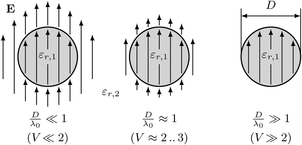
Fig. 2. Illustration of the E-field distribution E of the fundamental mode HE11 in a DWG at different wavelengths λ0 related to its diameter D.
Attenuation constant
The attenuation constant α(ω) of DWGs depends not only on the materials used for core and cladding, but also on the field distribution in both regions. For circular DWGs, the attenuation constant can be calculated by

where tanδ1, tanδ2 are the material loss factors and R 1, R 2 are the geometric loss factors of core and cladding, respectively [Reference Yeh and Shimabukuro19] (pp. 339), with

The geometric loss factors R 1 and R 2 represent the ratio between the power dissipation due to dielectric losses and the time-average power flow in core and cladding, respectively. E1, H1 and E2, H2 are the electric and magnetic vector fields of the fundamental mode HE11 in the core area A 1 and in the cladding area A 2, respectively. Both geometric loss factors R 1, R 2 can by normalized with respect to V and Δ. Their respective values have been analytically calculated from the numerical solution of the dispersion relation for circular DWGs as described in [Reference Yeh and Shimabukuro19] (pp. 137). The obtained values for R 1 and R 2 are shown in Fig. 3(a) in dependency of the normalized frequency V for typical material ratios of Δ in the mm-frequency range. It can be seen that with increasing frequency the proportion of the wave in the core region increases (R 1 increases, R 2 decreases). Since the cladding material has a lower permittivity than the core material, and thus usually a lower loss factor, it seems desirable to design DWGs with the lowest possible values of R 1 and the highest possible values of R 2. However, for low values of R 1 waves are weakly guided by the DWG which leads to unwanted radiation or mode coupling in case of discontinuities like bends. For this reason, higher values of R 1 ($V \approx 2$ –3) in combination with low-loss core materials are preferred in mm-wave applications.

Fig. 3. Geometric loss factors R 1, R 2 (a) and their respective derivatives dR 1/dV, dR 2/dV (b) as a function of the normalized frequency V for different material ratios Δ.
From (10) and (14), the Taylor coefficient α0 at a certain frequency $V_0 = V( \omega _0) = ( {\omega _0}/{c_0}) ( {D}/{2}) \sqrt {\varepsilon _{r, 1} - \varepsilon _{r, 2}}$ and therefore the attenuation of a DWG ($20\log ( e^{\alpha _0 l})$
 in dB) can be calculated by

Following the same procedure the Taylor coefficient α1 and therefore the change of the attenuation over frequency can by calculated by

It can be seen that α1 depends not only on the geometric loss factors R 1 and R 2, but also on their derivatives dR 1/dV and dR 2/dV. The derivatives for typical material ratios Δ are shown in Fig. 3(b) as a function of the normalized frequency V. Due to the negative values of the derivative of R 2, it seems possible to compensate for the frequency-dependent attenuation by appropriate material selection. However, such a minimization of α1 can only be achieved with a loss factor of the cladding material (tan δ2) significantly higher than the loss factor of the core (tan δ1) for typical material ratios Δ in the mm-wave frequency range. This would lead to a considerably higher insertion loss of the DWG. For this reason, α1 is significantly influenced by the permittivity and loss factor of the DWG core in practice.
With the help of (16) and (17) as well as Figs 3(a) and 3(b), the Taylor coefficients α0 and α1 can be directly calculated for a wide range of DWGs in the mm-wave frequency range. In Table 1 these coefficients are given exemplarily for single-mode DWGs (V 0 = 2.4) with air cladding (ɛr,2 = 1, tan δ2 = 0) and cores made of Teflon (PTFE), polyethylene (PE), and polystyrene (PS). Comparing the PTFE and the PE waveguide, it can be seen that the higher core permittivity of PE not only increases the transmission losses (e.g. from $3.1$ to 3.5 dB/m at 140 GHz), it also increases their frequency dependency. In combination with a high loss tangent (see PS in Table 1), the frequency dependency is highly increased. Since it is still unclear how this frequency dependency affects a signal transmitted via DWG, the coefficients α0 and α1 are used in Section “Signal distortions” to calculate the signal distortions caused by the frequency-dependent attenuation of circular DWGs.
Table 1. Taylor coefficients α0 and α1 as well as β0, β1, and β2 for some exemplarily chosen DWGs with air cladding (ɛr,2 = 1, tanδ2 = 0)

Phase constant
Similar to the attenuation constant α(ω) the phase constant β(ω) depends on the materials and field distributions in core and cladding. The phase constant is given by

where λg is the guided wavelength and ɛr,eff is the effective relative permittivity with ɛr,2 ≤ ɛr,eff ≤ ɛr,1. The effective relative permittivity is normalized by

which is referred as the normalized phase constant that ranges between values of 0 and 1 [Reference Yeh and Shimabukuro19] (p. 61). The normalized phase constant B can be used as a measure of the field concentration in core and cladding. It is shown as a function of the normalized frequency V for different values of Δ in Fig. 4(a). From (11), (18), and (19), the Taylor coefficient β0 at a certain normalized frequency V 0 and therefore the phase change per unit length at the center frequency ω0 can be calculated by

Following the same procedure the Taylor coefficient β1, namely the group delay per unit length, can by calculated by


By multiplying the derivative of β with diameter D, a normalized value for the first-order frequency dependency of the phase constant is obtained which only depends on V and Δ. This value is shown as a function of V for different values of Δ in Fig. 4(b). From (21) and Fig. 4(b) it can be seen that β1 and therefore the group delay τg varies strongly over frequency. In case of a broadband signal that is transmitted along such a waveguide, the different frequency components of this signal reach the receiver at different times. This effect is known as waveguide dispersion. To reduce the waveguide dispersion, the group delay should therefore be flat over frequency. According to Fig. 4(b) this is only possible for certain normalized frequencies in a range of 2 < V < 3 or V → ∞.

Fig. 4. Normalized phase constant B (a) as well as the first and second derivatives D(dβ/dV) (b) and D(d 2β/dV 2) (c) as a function of the normalized frequency V for different material ratios Δ.
The waveguide dispersion per unit length of a DWG is described by the Taylor coefficient


that has been derived from (11), (18), and (19). Multiplying the second derivative of β with diameter D yields a normalized value for the second order frequency dependency which only depends on V and Δ (shown in Fig. 4(c)). By using (20)–(22) as well as Fig. 4(a)–4(c), the Taylor coefficients β0, β1, and β2 can now be directly calculated for a wide range of DWGs in the mm-wave frequency range. From (22) and Fig. 4(c) it can be seen that the dispersion vanishes completely (β2 = 0) for certain DWG designs. Thus, it is possible to realize dispersion-minimized circular DWGs in the normalized frequency range 2.5 < V < 2.8. Air-clad PTFE waveguides, for example, with core diameters of D = 3.13 mm, D = 1.79 mm, and D = 1.04 mm have negligible dispersion at 80 GHz, 140 GHz, and 240 GHz, respectively (V = 2.62, Δ = 1) (see Table I). Due to the rounded diameter values, the dispersion minimum is not precisely obtained, but a comparison between the single-mode DWGs and the dispersion-optimized DWG in Table I shows that the Taylor coefficient β2 is considerably lower. It can be observed that dispersion-minimized designs are all multi-mode waveguides (V ≥ 2.405). In order to benefit from the low waveguide dispersion, it might be necessary to reduce the modal dispersion of these DWGs as described in [Reference Meyer, Turan and Schneider20]. However, one might also ask the question whether it is necessary to reduce the dispersion β2 to zero to obtain negligible signal distortions. For this reason, the Taylor coefficient β2 is used in Section “Signal distortions” to calculate the signal distortions caused by waveguide dispersion of circular DWGs.
Signal distortions
According to Heaviside [Reference Heaviside21] a channel is considered free of distortion if its propagation constant fulfills

Since this condition cannot be fulfilled by a DWG, the distortions to be expected when transmitting a signal via DWG are analyzed in the following. To evaluate DWGs as communication channels, the baseband (ω0 = 0) channel impulse response h(t) is used. The baseband impulse response can be determined by inverse Fourier transformation ${\large{\cal F}^{-1}}$ of the baseband frequency transfer function

where γ0, γ1, and γ2 are the complex coefficients of the approximated propagation constant $\tilde {\gamma }( \omega )$ given in (9). As described in Section “Data transmission system,” a band-limited signal is assumed that is caused by an ideal low-pass filter as transmit and receive filter (see equation (2)). Thus, the baseband impulse response is

For an analytical description of the impulse response h(t), the solution of (25) is separated into two parts. First, only distortions caused by a frequency-dependent attenuation are taken into account. In the second part, distortions due to a frequency-dependent phase constant, namely the dispersion, are considered.
Distortions caused by attenuation
The frequency-dependent attenuation of DWGs is modeled by the Taylor coefficients α0 and α1. Therefore, the baseband frequency response of the DWG given in (24) simplifies to

By applying the inverse Fourier transform according to (25), the baseband impulse response of the DWG channel is obtained:

This impulse response can now be used to determine the SNR and the ISI caused by the frequency-dependent attenuation of a DWG. For this considerations the Taylor coefficient β1 is set to zero, since it only represents a time shift (namely by the group delay τg) of the impulse response h(t) and, therefore, does not affect SNR and ISI.
Following equation (4) the SNR depends on the magnitude squared of the impulse response of the wanted signal |h(0)|2. For a DWG channel with frequency-dependent attenuation follows:

Since α1 l ωN is much smaller than 1 for DWGs in the mm-wave frequency range (see Section “Attenuation constant,”) the small argument approximation of hyperbolic sine (sinh(x) ≈ x) can be applied. Thus, the SNR simplifies to

This clearly shows that the SNR at the receiver of a DWG-based transmission system is simply the SNR of a channel with purely additive white Gaussian-distributed noise (AWGN channel) reduced by the attenuation of the DWG. Thus, the effect of the frequency-dependent attenuation on the SNR is negligible.
In addition to the SNR, the ISI is of interest in order to determine the expected signal distortions along the transmission channel. Applying the definition of the ISI given by (5) leads to an analytical description of the ISI. The magnitude squared of the impulse response of the wanted signal |h(0)|2 has already been given by (28). The sum of the magnitude squared of the impulse response of all signals that superimpose the wanted signal converges to

(for derivation see Appendix A). Using (28) and (30) as well as the definition of the ISI given by (5) an analytical description of the ISI can be obtained:

Figure 5(a) shows the ISI for the common range of Taylor coefficient α1 in the mm-wave frequency range for different signal bandwidths 2f N and a DWG length of l = 1 m. It can be seen that for typical values of the frequency-dependent attenuation in the mm-frequency range $\alpha _1 = 10^{-13}\rm { {..}}\,10^{-11}$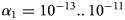 s/m a tolerable ISI can be achieved for all bandwidths over a DWG length of l = 1 m. For example, the single-mode DWG made of PTFE given in Table I of 1 m length would still achieve a very good ISI of 33 dB even at a bandwidth of 20 GHz. Using a single-mode DWG made of PS reduces the ISI to 17 dB due to higher frequency dependency of the attenuation. With increasing length, the signal distortions further increase. For example, if the length is changed from $1$
 to 10 m, the ISI lowers by 20 dB. Therefore, for larger bandwidths and longer length l an optimization of the DWG toward low α1 ≤ 10−12 s/m is recommended. A detailed study is given in Section “DWG design for low signal distortions.”

Fig. 5. ISI as a function of Taylor coefficient α1 (a) and β2 (b) for different signal bandwidths 2f N as well as α1 and β2 (c) at a signal bandwidth of 2f N = 5 GHz.
Distortions caused by dispersion
The frequency-dependent phase constant of DWGs is modeled by the Taylor coefficients β0, β1, and β2, which includes the modeling of group delay and dispersion. This yields the baseband frequency transfer function given by (24). Applying the inverse Fourier transform according to (25) leads to the impulse response of the dispersive DWG channel

where erf() represents the error function

Similar to Section “Distortions caused by attenuation,” the Taylor coefficient β1 is set to zero for further analysis, since it has no influence on the signal distortions. Accordingly, the magnitude squared of the wanted signal is

and the magnitude squared of the interfering signal is

with

The series (35) converges (for proof see Appendix B) and is therefore analyzed numerically to determine the ISI. First, the ISI is considered without the influence of frequency-dependent attenuation (α1 = 0). The results are shown in Fig. 5(b). A considerably greater effect on the ISI compared to the frequency-dependent attenuation can be observed in Fig. 5(a). Especially with increasing signal bandwidth the ISI increases significantly. For typical values of |β2| ≤ 10−21 s2/m2, an acceptable ISI can only be achieved for smaller bandwidth and/or shorter length. If the single-mode DWG made of PTFE in Table I is considered, it can be seen that for a bandwidth of 20 GHz and a length of 1 m only an ISI in a range of $\approx \! 10 { {..}}\,20\, {\rm dB}$ is achieved. This is a significant reduction compared to the ISI caused by frequency-dependent attenuation. A transmission over l ≥ 10 m seems only possible for smaller bandwidths (e.g. 5 GHz). However, as already shown in Section “Phase constant,” the waveguide dispersion can be reduced to almost zero (|β2| → 0) for certain circular DWGs. In this case, the ISI and therefore the transmission length would be infinite. Since in practical application, the frequency-dependent attenuation is not negligible (see Section “Distortions caused by attenuation”), the question remains whether a minimized waveguide dispersion actually results in a low overall ISI.
DWG design for low signal distortions
As shown in Sections “Distortions caused by attenuation” and “Distortions caused by dispersion,” frequency-dependent attenuation as well as waveguide dispersion have a significant effect on signals transmitted along a DWG. This is especially true for long distance communications (l ≥ 10 m). However, it has also been shown that for certain circular DWGs, the waveguide dispersion vanishes completely (β2 = 0). An interesting question at this point is whether this dispersion minimum really leads to minimal signal distortions despite frequency-dependent attenuation (α1 ≠ 0). To answer this question, equation (35) is evaluated numerically for values of α1 ≠ 0. In order to keep the variation of the results low, only a bandwidth of 2f N = 5 GHz is considered. The results for the ISI in dependency of α1 and β2 are shown in Fig. 5(c). It can be seen that for small values of α1 (≤ 10−15 s/m) the ISI as a function of α1 and β2 in Fig. 5(c) is almost congruent with the ISI in Fig. 5(b) (B = 5 GHz), where only dispersion caused by frequency-dependent group delay (α1 = 0) is considered. The influence of the frequency-dependent attenuation on the ISI can therefore be neglected for α1 ≤ 10−15 s/m. With increasing values of α1, however, a limitation in the maximum achievable ISI appears despite negligible waveguide dispersion (β2 ≤ 10−25 s2/m2). For example, a DWG with a Taylor coefficient of α1 = 10−12 s/m and 1 m length leads to an ISI of ISI ≈ 41 dB even if the waveguide dispersion is zero. This limitation in the maximum achievable ISI despite negligible waveguide dispersion corresponds to the values determined for the attenuation-dependent ISI in Fig. 5(a) (B = 5 GHz). Whether the optimization of a DWG to low waveguide dispersion also leads to a reduction of the expected ISI depends mainly on the frequency-dependent attenuation of the respective DWG. For example, for a DWG with a Taylor coefficient of α1 = 10−12 s/m, reducing the waveguide dispersion below |β2| ≤ 3 × 10⁻²³ s2/m2 would not further improve the ISI. This clearly shows that low signal distortions in DWGs can only be achieved if the frequency-dependent attenuation in addition to dispersion is reduced. This fact has not been considered in the majority of scientific studies so far. Furthermore, it is more challenging to reduce the frequency dependency of the attenuation than to reduce the waveguide dispersion of a DWG. Considering the mathematical description of the first-order frequency-dependent attenuation in (17), it is noticeable that the loss factors of core and cladding (tanδ1, tanδ2) occur with different prefactors. If both factors are considered separately, it can be seen that the prefactor of the cladding material's loss factor becomes negative for normalized frequencies of V ≥ 1.2 (see Fig. 6). Thus, a minimization of the Taylor coefficient α1 to zero is theoretically possible. However, a reduction of the frequency dependency of the attenuation is only possible if the cladding material has significantly higher losses than the core material ($\tan \delta _2\approx 4\,{ {..}}\,5\times \tan \delta _1$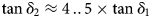 ). This would result in a significant increase of the total losses of the DWG and thus in a decrease of the SNR at the receiver.
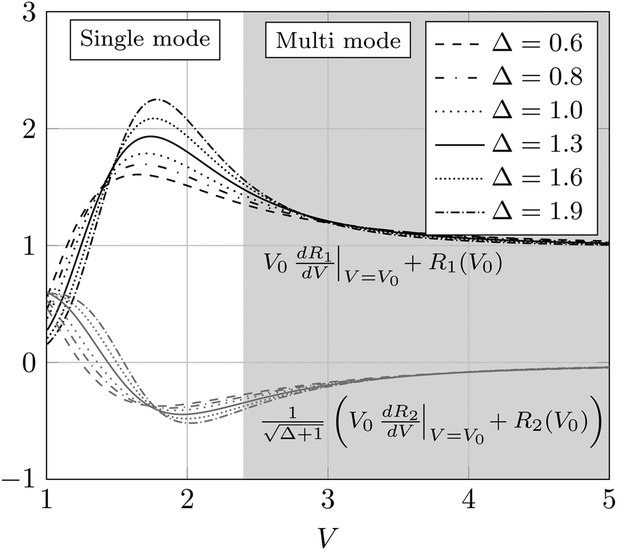
Fig. 6. Core and cladding material prefactor in (17) as a function of the normalized frequency V for different material ratios Δ.
It can generally be said that for low material ratios Δ the frequency dependency of attenuation and group delay is reduced and the signal distortions decrease. However, lower values of Δ also result in a lower field concentration in the core of the DWG (see Fig. 3(a)). This requires a larger size of the DWG package (core + cladding). In addition, the sensitivity to discontinuities will be increased. Therefore, a compromise on practical issues must be found when reducing Δ. In most of nowadays DWG applications, the relative permittivity of the used materials is in a range of $\varepsilon _r \approx 2 { {-}}3$ and the loss factor in a range of $\tan \delta \approx 10^{-4} { {-}}10^{-3}$
 . Considering (17) and Fig. 6, the respective range of this Taylor coefficient is $\alpha _1 \approx 10^{-13} { {-}}10^{-11}$
 s/m ($V \approx 2 { {-}}3$
 ). For such DWGs, a minimization of the waveguide dispersion is recommended, since it also reduces the frequency-dependent attenuation to an acceptable value. For the waveguide-dispersion-minimized DWG in Table I with a Taylor coefficient of α1 = 6.0 × 10⁻¹³ s/m, an ISI of ISI = 10 dB could still be achieved over lengths of 58 m (5 GHz bandwidth) or 14 m (20 GHz bandwidth). Reducing α1 by a factor of 10 allows to increase the respective lengths by the same factor. For comparison, using the single-mode DWG made of PTFE in Table I with Taylor coefficients of α1 = 6.4 × 10⁻¹³ s/m and β2 = 2.0 × 10⁻²² s/m would only achieve a transmission length of 19 m (5 GHz bandwidth) or 1.3 m (20 GHz bandwidth). This clearly shows the great potential of dispersion optimization of DWGs in the mm-wave frequency range.
Conclusion
In this paper, a detailed study of signal distortions due to frequency-dependent attenuation and group delay of DWGs in a low-complexity digital transmission system was presented. Based on a general description of this frequency dependency for circular DWGs, it was shown that both frequency-dependent attenuation as well as waveguide dispersion have a significant effect on the signal transmission. Although it is possible to reduce the waveguide dispersion to zero by proper waveguide design, the remaining frequency-dependent attenuation significantly limits the transmission capacity. It has also been shown that a complete compensation of this effect is only feasible if the cladding material of the DWG shows significantly higher losses than the core material. With the currently available materials, this would result in high transmission losses. However, reducing the frequency-dependent attenuation to an acceptable level can be achieved with the currently available materials, especially for dispersion-minimized DWGs. For this purpose, it is recommended to choose a core material with low permittivity and low losses (e.g. PTFE and PE) and at the same time a low material ratio Δ. Such improvements of the transmission channel allow to further reduce signal distortions and thus to further increase the maximum achievable data rates and transmission distances without the need of more complex transceivers.
Appendix A. Derivation of ISI caused by frequency-dependent attenuation
The ISI caused by a frequency-dependent attenuation of a DWG is defined by (5) with (28) in the numerator and the infinite sum

in the denominator. This denominator can be rewritten as

where |h(0)|2 is given by (28) and

Thus

Consequently, for the ISI follows

Appendix B. Convergence of ISI caused by dispersion
To proof that the ISI caused by frequency-dependent attenuation and frequency-dependent group delay of a DWG can be calculated numerically, as it has been done in Section “Signal distortions,” it is needed to proof its convergence. The ISI under influence of dispersion is defined by (5) with (34) in the numerator and (35) in the denominator. To verify that the infinite series in (35) converges, the series is first divided into two sums, each with a positive running index k. Afterward, the convergence of both sums is verified separately:

The convergence of both sums in (B.1) can be verified by the comparison test which states that an infinite series $\sum _{n = 0}^{\infty } a_n$ converges, if there is a convergent infinite series $\sum _{n = 0}^{\infty } b_n$
 for whose real summands holds: |a n| ≤ |b n| for all $n\geq n_0 \in {\opf N}$
 , where n 0 can be any countable running index.
Using the triangle inequality

and the asymptotic expression of the error function [Reference Zwillinger, Moll, Gradshteyn and Ryzhik22]

it can be stated for the summands of the first sum in (B.1) that

In order to fulfill the comparison test, it is necessary to verify whether the sum

actually converges. This can be verified by the ratio test which states that an infinite series $\sum _{n = 0}^{\infty } b_n$ converges if its summands satisfy: |(b n+1)/(b n)| < 1 for $n \geq n_0 \in {\opf N}$
 . Thus,

with


Equation (B.6) simplifies to

It can be directly seen that with increasing running index k the numerator in (B.11) decreases faster than the denominator. Thus, the series (B.5) must have a non-countable set of summands with the running index k > k 0 that fulfill condition (B.11). As a result, the series (B.5) and therefore the first sum in (B.1) converges. Since the proof given for the first sum in (B.1) also holds for the second sum, equation (B.1) converges. Obviously, the convergence of series (B.1) is also valid for the case α1 = 0, as used in Section “Distortions caused by dispersion.”
 Andre Meyer received his Diploma degree in Communication and Information Technology from the University of Bremen, Germany in 2015. He is currently a research engineer at the RF & Microwave Engineering Laboratory of the University of Bremen, working toward his Ph.D. degree in high data-rate transmission systems using dielectric waveguides.
 Martin Schneider received his Diploma and Doctorate degree in Electrical Engineering from the University Hanover, Germany, in 1992 and 1997, respectively. From 1997 to 1999, he was with Bosch Telecom GmbH, where he developed microwave components for point-to-point and point-to-multipoint radio link systems. In November 1999, he joined the Corporate Research division of Robert Bosch GmbH. As a project and section manager of the “Wireless Systems” group he focused on research and development of smart antenna concepts for automotive radar sensors at 24 and 77 GHz. From 2005 to 2006, he was with the business unit “Automotive Electronics” of Robert Bosch GmbH where he was responsible for the “RF electronics” of automotive radar sensors. Since March 2006, he has been a full professor and head of the RF & Microwave Engineering Laboratory at the University of Bremen (Germany).


 Open access