

Abstract
The development of the high-temperature superconductors (HTS) has allowed the emergence of diverse superconductor devices. Some of these devices, like wind power generators and high-field magnets, are classified as large-scale HTS systems, because they are made of several hundreds or thousands of turns of conductors. The electromagnetic analysis of such systems cannot be addressed by means of the available analytical models. The finite-element method has been extensively used to solve the H formulation of the Maxwell's equations, thus far with great success. Nevertheless, its application to large scale HTS systems is still hindered by excessive computational load. The recently proposed T-A formulation has allowed building more efficient models for systems made of HTS tapes. Both formulations have been successfully applied in conjunction with the homogenization and multi-scaling methods, these advanced methods allow reducing the required computational resources. A new advanced method, called densification, is proposed here. The most important contribution of this article is the comprehensive comparison of the strategies emerged from the combined use of the two formulations and the three advanced methods.
Export citation and abstract BibTeX RIS

Original content from this work may be used under the terms of the Creative Commons Attribution 4.0 license. Any further distribution of this work must maintain attribution to the author(s) and the title of the work, journal citation and DOI.
1. Introduction
More than three decades after the discovery of the first high temperature superconductor (HTS) with a critical temperature above the boiling point of nitrogen, the technology has matured and the second-generation of HTS (2G HTS) conductors are now commercially available with practical length and critical currents [1–3]. 2G HTS conductors are layered composites with a thin layer of HTS material. 2G HTS conductors are also called 2G HTS wires, coated conductors (CC), or (RE)BCO tapes for instance. For simplicity, the term HTS tapes is used in this article.
The emergence of HTS tapes has favored the development of diverse superconductor devices. For power systems, it is expected that cables and fault current limiters will soon reach market maturity [4]. Continuous research and development have targeted other power devices, such as transformers, generators, and superconducting magnetic energy storage systems [5–7]. For scientific and medical applications, the interest in the technology has spawned over magnetic resonance imaging (MRI) and nuclear magnetic resonance (NMR) magnets [8, 9] and high magnetic field magnets [10]. These devices are typically made of hundreds or even thousands of turns of HTS tapes. Because of the large number of turns, these devices are classified as large-scale HTS systems [11–13].
To ensure safe operation, the design of HTS devices must consider effects that arise from changes in external magnetic field and transport current. During these changes, hysteresis losses are generated in the HTS materials, which under extreme cases lead to the loss of the superconducting state [13–15]. For simplicity in this article, the hysteresis losses are simply referred to as losses. The estimation of current density, electric and magnetic fields inside the superconductor is a mandatory step for obtaining the losses [16], as well as other quantities of interest for practical applications, such as the screening current-induced field and the field drift [8, 17–19].
The available analytical models are restricted to the analysis of individual tapes or relatively simple assemblies under restrictive conditions [20–26]. The analysis of systems with more intricate geometries and operating conditions, i.e. real HTS systems, requires the use of numerical methods [14, 27–33]. One of these methods is the finite element method (FEM) which is well documented in the literature [34–36] and has been extensively used to address the analysis of HTS systems. Maxwell's equations can be written using different formulations. The formulations differ from each other in the selection of the state variables. The most frequently used formulations within the superconductor community, are: A-V formulation [16, 37–39], T-
 formulation [40, 41], and H formulation [42–44].
The H formulation as used nowadays was introduced in [42, 43]. This formulation has been widely used during the last years and has arguably become the de facto standard within the applied superconductivity community. Recently published reviews [45, 46] claim that the H formulation has been used by more than 45 research groups worldwide. However, the use of the H formulation to analyze large-scale systems can become easily prohibitive in terms of computational load if one considers each individual turn/tape of the large-scale system in detail. The models considering in detail all the tapes of the system are referred to as H full models.
The T-A formulation which was proposed in [47, 48] has allowed building more efficient models than those based on the H formulation. In this formulation, the HTS tapes are modeled as infinitely thin lines, therefore the mesh complexity and the computation time can be significantly reduced.
The limitations of the full models have favored the emergence of approaches like the homogenization and multi-scaling methods. In this article, we call all these approaches advanced methods, because they represent an advancement with respect to simulating in detail all the turns of the system. The homogenization assumes that a stack made of HTS tapes can be represented by a single anisotropic homogeneous bulk [15]. The multi-scaling method is based on the analysis of a reduced set of tapes, called analyzed tapes, and the subsequent approximation of the behavior of the full system [13]. As of today, these two advanced methods have been successfully used together with the H and T-A formulation, giving rise to the following strategies: H homogeneous [15], H multi-scale [13], H iterative multi-scale [49], T-A homogeneous [50], and T-A simultaneous multi-scale [50]. The H multi-scale and H iterative multi-scale strategies require two submodels which are used to separately compute the background magnetic field and the current density. The T-A simultaneous multi-scale strategy requires just one model and computes the magnetic field and the current density simultaneously. In the [50] the T-A simultaneous multi-scale strategy is called just T-A multi-scale, here the adjective 'simultaneous' is added to differentiate this strategy from the multi-scale and iterative multi-scale strategies.
The first contribution of this article is the presentation of new strategies. A new advanced method, called densification, is proposed here thereby giving rise to the H densified and T-A densified strategies. The densification method consists in merging together some tapes of a stack of tapes, so that the original stack can be modeled by means of fewer tapes. The ideas of the multi-scaling method are revisited and the H simultaneous multi-scale strategy is proposed. The H and T-A simultaneous multi-scale strategies are enhanced by means of the homogenization and densification of the non-analyzed tapes, resulting in four additional strategies. Figure 1 shows a tree diagram with the different strategies that emerge from the combination of the H and T-A formulations, and the advanced methods. The blue rectangles represent the strategies already described in the literature, while the green rectangles stand for the strategies that are original contributions of this article. The second and most important contribution of this article is the comprehensive comparison of the strategies showed in figure 1.
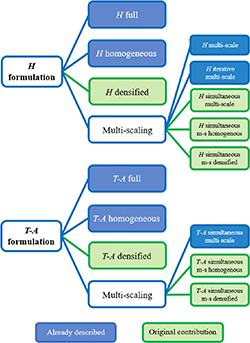
Figure 1. Tree diagram showing the strategies that emerge from the coupling of the formulations: H and T-A; and the advanced methods: homogenization, densification, and multi-scaling. The strategies already described in the literature are represented by blue rectangles, while the strategies that are original contributions are represented by green rectangles.
Download figure:
Standard image High-resolution imageThe models presented in this article were implemented in COMSOL Multiphysics 5.3 [51]. The implementation of the H multi-scale and H iterative multi-scale strategies require the use of two COMSOL models that are called by a MATLAB script. The computer used to perform the simulations is an Apple MacBookPro (3 GHz Intel Core i7-4578 U, 4 cores, 16 GB of RAM). The characteristics of the computer are important to compare the reported computation times.
This article is organized as follows. Section 2 contains a brief description of the H and T-A formulations. The case study used to compare the strategies is presented in section 3, the reference and full models are also presented in the same section. The strategies coupling the H formulation and the advanced methods are described in section 4, the strategies and their respective models are presented first, and the simulation results are presented together at the end of this section to facilitate their comparison. The strategies coupling the H and T-A formulations and the advanced methods are described in sections 4 and 5, respectively. The strategies and their respective models are presented first, and the simulation results are presented together at the end of each section to facilitate their comparison. Section 6 contains the comparison and discussion of the different strategies. An assessment of the ease with which the models can be built is presented in section 7. Finally, the conclusions are presented in section 8.
2. Formulations
In this section, salient information of the H and T-A formulations are briefly recalled. For further information related to the H formulation, the reader is referred to [42, 45]. For further information related to the T-A formulation, the reader is referred to [47, 48].
2.1. H formulation
The H formulation uses the magnetic field strength  as dependent variable. Within a bounded universe the different materials are represented by different subdomains. Each subdomain has different properties, i.e. resistivity
  and permeability
  . These values define the constitutive relations
  and
and  , where
  and
and  are the electric and magnetic field strength, respectively, and
  and
and  are the magnetic flux and current density, respectively.
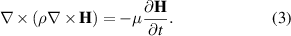
To derive the governing equation of the H formulation, Ampère's law is written neglecting the displacement current. Then, Ampère's and Faraday's laws are given by

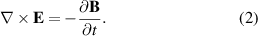
If we consider just linear magnetic materials ( ), equations (1) and (2) yield the governing equation of the H formulation
Gauss's law  is fulfilled by means of the election of the initial conditions,
  , as explained in [15, 42].
Figure 2 depicts a two-dimensional (2D) planar model, where the x–y plane contains the cross-section of the superconductors. The subdomains  ,
,  , and
, and  represent the superconductor, normal conductor and surrounding mediums, respectively. The surrounding medium subdomain includes the insulating materials and the cryogenic liquid. In the 2D planar model,
  has two non-zero components
  , while
 and
and  have just one non-zero component each
  .
.
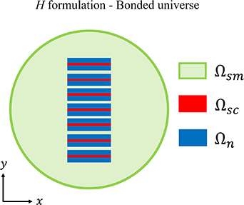
Figure 2. Bounded universe of the H formulation 2D planar model, formed by the union of the superconductor  , normal conductor
  , and surrounding medium
  subdomains.
Download figure:
Standard image High-resolution imageThe transport currents  in each conductor are imposed by means of integral constraints. One constraint is required for each conductor, as explained in [15, 42].
The selection of the elements used in the FEM discretization plays also an important role on the accuracy and computational speed of the numerical model. In the case of the H formulation, several arguments are presented in [15, 42, 52] showing the advantages of the first-order edge elements over other kind of elements.
2.2. T-A formulation
The T-A formulation, as described in [47, 48], relies on the primary assumption that the thin superconducting layers of the HTS tapes can be modeled as one dimensional (1D) objects in a 2D model. The infinitely thin approximation is meaningful when dealing with superconductors wires having large aspect ratio (width/thickness), like the 2G HTS tapes, where this ratio is in the range of  [1]. The T-A formulation requires the implementation of both the T and the A formulations, and both state variables
  and
and  , current and magnetic vector potentials, are evaluated.
Here, a 2D planar geometry is assumed, as illustrated in figure 3. The bounded universe is made of 1D superconducting layers and the surrounding medium  . The normal conductor layers of the HTS tapes are not considered. It is assumed that the current only flows through the superconducting layers, and the surrounding medium is assumed to be non-conductive. The current vector potential
  is exclusively defined over the superconducting layers, while the magnetic vector potential
  is defined over the entire bounded universe.
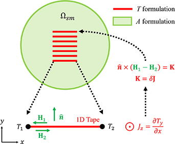
Figure 3. Bounded universe of the T-A formulation consisting of superconducting 1D layers and a surrounding medium.  is computed over the superconducting 1D layers and
  is computed over the entire bounded universe.
Download figure:
Standard image High-resolution imageFaraday's law (equation (2)) and the definition of the current vector potential  ) are used to derive the governing equation of the T formulation
In the 2D case depicted in figure 3, as long as the thickness of the superconducting layer can be neglected,  and
and  have only one non-zero component
  , and equation (4) is simplified as follows:
The transport currents in each tape  are imposed by setting the boundary conditions for
  . The values of
  at the edges of the 1D layer (
 and
and  ) must fulfill the following relation

where  is the real thickness of the HTS layer. Usually,
  or
or  is set to zero, and the other value is computed by means of equation (6).
The component of B perpendicular to the superconducting layer  , required to compute
  in equation (5), is obtained by calculating
  . Ampère's law (equation (1)) and the definition of the magnetic vector potential
 are used to derive the governing equation of the A formulation

In 2D cases,  is the only non-zero component of
  , therefore equation (7) is simplified to
  . At first glance, equation (7) should be simplified to
  . However, as the current flows only through the 1D superconducting layers,
  is zero all over the bounded universe, and the current is imposed by means of boundary conditions.
Thus, in order to couple  with the A formulation, the surface current density
  is introduced as

In the 2D case depicted in figure 3,  .
.
As previously mentioned,  is then imposed into the A formulation as an external surface current density by means of boundary conditions of the form

where  is the unit vector normal to the tape, and
  and
and  are the magnetic field strength vectors above and below the HTS layer, respectively.
As in the case of the H formulation, the selection of the elements used in the FEM matters. Two kind of elements are required, Lagrange second-order elements are used to approximate  and Lagrange first-order elements for
  . These specific choices avoid spurious solutions, as justified in [50].
3. Case study and full models
3.1. Case study
The case study used in this work is the same racetrack coil presented in [13, 50]. This coil has ten pancakes, each consisting of 200 turns, bringing a total number of turns equal to 2000. The transport current in each turn is the same, because they are connected in series. The geometric parameters of the coil are recalled in table 1. A unit cell is defined as the rectangular region occupied by a tape and its immediate surrounding medium. It is considered that the winding of the coil is even, thus all the unit cells have the same dimensions. The symmetry of the coil allows modeling just one quarter of the coil's cross-section. Therefore, it is possible to consider only five stacks, each consisting of 100 turns in a planar 2D geometry. The coil, its cross-section and the modeled section are depicted in figure 4.

Figure 4. The racetrack coil used as case study has ten pancakes with 200 turns per pancake. The coil can be modeled by means of only 1/4 of the coil's cross-section. The mesh in the unit cells is structured. The unit cell includes the tape and its surrounding medium. The reference model considers 100 elements along the tapes' width, while the H full and T-A full models consider 60 elements.
Download figure:
Standard image High-resolution imageTable 1. Case study geometric parameters.
| Parameter | Value |
|---|---|
| Number of pancakes | 10 |
| Turns per pancake | 200 |
| Unit cell width | 4.45 mm |
| Unit cell thickness | 293 
|
| HTS layer width | 4 mm |
HTS layer thickness 
| 1 
|
The constitutive  relation of the HTS material is modeled by the power-law [53], therefore the resistivity of the superconducting subdomains
  is given by
The Kim-like model [14, 54] is used to describe the anisotropic behavior of the HTS tapes, so that  is defined by
where  and
and  are the magnetic flux density components perpendicular and parallel to the wide surface of the tape, respectively. The parameters of equations (10) and (11) are summarized in table 2.
Table 2. Case study electromagnetic parameters.
| Parameter | Value |
|---|---|

|
|

|

|

|
|

|

|

|

|

|

|
3.2. Reference model
The H formulation model that considers in detail each individual tape, presented in [13, 50], is used in this article to validate the rest of the models, and it is hereinafter called reference model.
The HTS tapes are composed by one layer of superconductor and different layers of normal conductors e.g. copper, silver, substrate [1]. The resistivity of the superconducting layer is several orders of magnitude lower than the resistivity of the other normal conductor layers forming part of the HTS tapes [15]. Therefore, the reference model does not include any normal conductor subdomain  . The resistivity of the surrounding medium subdomain
  is considered to be
  [15]. No magnetic materials are considered, then the permeabilities of the superconducting
  and surrounding medium
  subdomains are equal to the permeability of vacuum
  .
.
Figure 4 depicts the geometry of the reference model including the numbering of pancakes and tapes. The mesh of the unit cells is structured with one element along the HTS layers' thickness and 100 elements along their width. An increasing number of elements towards the edges of the tapes allows increasing the accuracy of the  distribution in the regions where the magnetic field penetrates the tapes [13].
3.3. H and T-A full models
An assessment of the number of elements along the tapes' width was presented in [50]. The results demonstrated that, for the test conditions (transport current of 11  , and 50
 , the compromise between accuracy and computation time is fulfilled with 60 elements. The H formulation model that considers in detail each tape of the system and uses 60 elements along the tapes' width is hereinafter called H full model. The mesh of the unit cells of the H full model is also presented in figure 4. Accordingly, the difference between the reference and the H full models is the distribution and the number of elements along the tapes' width, 100 elements with a non-uniform distribution for the reference model, and 60 elements with a uniform distribution for the H full model. In addition, throughout the rest of this work, it is assumed that all models have 60 elements along the tapes' width, with the exception of the reference model. The presentation of the H full model with 60 elements is relevant to compare the computation times and decide which reductions are due to the number of elements and which reductions are due to the choice of the strategy.
The T-A full model uses the T-A formulation, and as well as the reference and H full models, considers in detail all the tapes. Specifically, in the case of the T-A formulation models, 'considers in detail all the tapes' means that the current vector potential  is computed along every single-tape. The mesh of the unit cells is also structured as shown in figure 4. In this case, the HTS layers have no thickness and the mesh is made of 1D elements uniformly distributed along the HTS layers' width.
3.4. Results
The reference, H full and T-A full models were simulated for one cycle of a sinusoidal transport current with an amplitude of 11  , and a frequency of 50
 . The value 11
  was chosen because at the peak of the cycle the tape 1 of pancake 5 is completely penetrated by the current density. The simulation results are compiled in figure 5, in tabular format. The first column contains the normalized current density
  . The magnitude of the magnetic flux density
  is presented in the second column. The plots of these first two columns show the results at the first negative peak of the transport current
  . It can be seen that both the
  and
and  plots are indistinguishable to the naked eye between the different formulations.
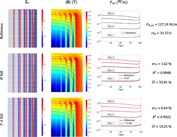
Figure 5. Results of the reference, H full, and T-A full models. The first and second columns show  and
and  at the first negative peak of the transport current
  . The third column shows the average losses as a function of the tapes' location inside each pancake. The tapes and pancakes are numbered as indicated in figure 4.
Download figure:
Standard image High-resolution imageThe third column of figure 5 contains the average losses plots. The x-axis in these plots represents the tapes' number. There are five curves in each plot, one for each pancake. The numbering of the tapes and pancakes follows the order presented in figure 4. The losses estimated with the H and T-A full models are very similar to those estimated with the reference model, but there are visible differences, particularly in the first two pancakes. Due to the higher current penetration, the losses in pancake 5 are almost three orders of magnitude larger than the losses in pancake 1. Although there are variations in the losses at the end of the pancakes, the losses in a given pancake remain within the same order of magnitude.
The quantitative comparison of the models is carried out by calculating the relative error of the average losses, the coefficient of determination  of the
  distributions, and the normalized computation time. These data are listed in the fourth column of figure 5.
The average power losses are obtained using data of the second half of the cycle, as follows:
where  is the period of the sinusoidal cycle, and
  are the superconducting subdomains. In the 2D models addresses in this paper, the integral over
  is a surface integral, then the double integral symbol is preferred. The relative error of the average losses, expressed in percent, is defined as
where  and
and  are the average losses computed with the reference model and the model that is being compared, respectively. The previous definition allows for positive and negative errors to be computed. Therefore, it will be possible to know if a model overestimates (
 ) or underestimates (
 ) the losses. For the test conditions,
  .
.
Unlike the average losses which are scalars, the  distributions are multivariable functions. The coefficient of determination is a widely used metric to evaluate the goodness of the fit [55], here it is used to compare the
  distributions, and is defined as
where  and
and  are the
  distributions computed with the reference and tested models, respectively.
  is the mean value of
  . It must be remembered that
  means a perfect matching between
  and
and  . The coefficient
  has an advantage over the error
  . The averaging nature of
  tends to hide local and instantaneous errors, e.g. an instantaneous excess in the losses may be compensated by another instantaneous deficit; on the contrary, these same errors have a cumulative effect in
  .
.
The normalized computation time is defined as
where  and
and  are the computation times required by the reference model and the model that is being compared, respectively. For the test conditions,
  .
.
The results of the fourth column in figure 5 show that the accuracy of the H and T-A full models is satisfactory compared to the reference model. The errors  are lower than
  , and coefficients
  are larger than 0.98. The computation time are 17 h 36 min (
 ) and 3 h 14 min (
 ), for the H and T-A full models, respectively. These values, more specifically the normalized computation times, demonstrate that the T-A formulation allows building more efficient full models in term of computation time keeping a fairly good accuracy.
4. H formulation strategies
4.1. Homogenization
The homogenization method consists in modeling the stacks of HTS tapes as homogeneous bulks. When the stack is transformed into an anisotropic bulk its geometric features are 'washed out'. This process is depicted in figure 6. The model should include additional features that allow the electromagnetic behavior of the homogeneous bulk to resemble that of the original stack.
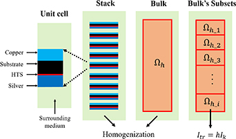
Figure 6. The homogenization process transforms a stack of HTS tapes into a homogeneous bulk. The bulk is subdivided into bulk's subsets  , one integral constraint is used to impose the transport current in each subset.
Download figure:
Standard image High-resolution imageThe non-superconducting materials forming part of the stack have resistivity values several orders of magnitude larger than those of the HTS material, hence only the HTS material resistivity is considered in the homogenization process. The resistivity of the bulk is derived from equations (10) and (11). But the  value must be replaced by a homogenized critical current density
  , defined as

where
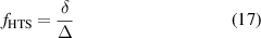
 is the real thickness of the HTS layer, and
  is the thickness of the unit cell. Thus, the superconducting properties of the HTS tapes are diluted in the cross-section of the bulk.
In the H full model, it is necessary to add one integral constraint per tape to impose the desired transport current. In the H homogenous model, the bulk subdomains  are further subdivided into bulk's subsets
  , as depicted in figure 6. Then, one constraint is necessary for each bulk's subset, instead of one constraint per tape. The transport current imposed in a given subset is
  , where
  is the transport current in the original tapes and
  is the number of tapes covered by the subset. The losses are computed in each bulk's subset. The losses in each subset are divided by the number of tapes included in each subset, then it is possible to approximate the losses along the stack. A detailed description of the H homogenous strategy can be consulted in [15].
The H homogenous model of the case study considers five bulks, one for each pancake. Each bulk is subdivided into six subsets, as shown in figure 7. The subsets in the upper part of the pancakes have a larger aspect ratio than the ones closer to the symmetry plane. Such kind of distributions has been recommended in [13, 15]. The mesh of the bulks is structured and considers one element along the subset's thickness and 60 elements along the tapes' width, as depicted in figure 7.

Figure 7. Geometry and mesh of the H and T-A homogeneous model. There are five bulks. Each bulk is subdivided into six subsets. The mesh of the bulks considers one element along the subsets' thickness and 60 elements along the tapes' width.
Download figure:
Standard image High-resolution image4.2. Densification
Unlike the homogenization and the multi-scaling methods, the densification method is an original contribution of this article. The densification method addresses the analysis of stacks by means of a reduced number of tapes, called densified tapes. The densified tapes merge a given number of tapes into a single tape. In the densification process, the densified tapes preserve their original geometry and concentrate the transport current of their surrounding tapes, while the surrounding tapes are erased.
The idea of the densification, as in the case of the homogenization, is to build models with a smaller number of elements. Nevertheless, the reduced number of elements should not compromise the accuracy of the models. In the densification the number of elements is reduced by means of a reduced number of densified tapes. In the homogenization the electromagnetic behavior of the original stack is preserved by means of the distribution of the transport current all over the bulks, here this requirement is met by means of the concentration of the transport current in the densified tapes.
As in the previous models, the densified model does not include the normal conductors forming part of the HTS tapes. The resistivity of superconducting subdomains of the densified tapes is derived from equations (10) and (11), where the  value is replaced by a densified critical current density
  defined as

where  is the number of tapes merged into a single densified tape.
The transport current in the densified tapes is  , where
  is the transport current in the original non-densified tapes. It is necessary to add one integral constraint per densified tape with the proper transport current
  . Then, as in the case of the H homogenous model, the number of constraints is reduced.
The densification process is depicted in figure 8. In this example, a given densified tape is built out of three tapes, labeled  ,
,  and
and  , therefore
  . The densified tape is located at the position of the original tape
  . It is not necessary for
  to be an integer. The parameter
  may be equal to other real positive number. For instance, a stack made of five tapes can be modeled by means of two densified tapes. In this case, the densified tapes may merge three and two tapes, respectively. In another possible scenario, the densified tapes may merge 2.5 tapes, then the parameter
  should be
  for both densified tapes.

Figure 8. Densification process, the number of tapes in the original stack is reduced and the transport current of the merged tapes is forced to flow in the densified tapes.
Download figure:
Standard image High-resolution imageOnce the  distribution is computed, the losses can be calculated in the densified tapes. The losses in the densified tapes are divided by their corresponding
  , and these values are used to interpolate the losses in each tape of the original stack.
The accuracy of the densified models may be degraded due to the nature of the densified tapes, larger self-fields and larger distances between tapes than in the full models. Therefore, the number and the position of the densified tapes must be carefully assessed. In order to build a successful H densified model of the case study, different sets of densified tapes were tried. According to our heuristic criterion, the compromise between accuracy and computation time is fulfilled with a set of 31 densified tapes per pancake. The geometry of the model and the position of the densified tapes are depicted in figure 9. The first 21 densified tapes merge four tapes each ( ). For the following four tapes, the parameter
  takes the values {3, 3, 2, 2}, respectively. Finally, for the upper six tapes
  , meaning that these six tapes are not densified. The distribution of densified tapes is denser at the upper part of the pancake than at the bottom to achieve the required accuracy in the regions where larger variations in the
  distributions arise.
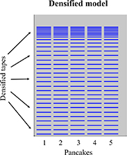
Figure 9. Geometry of the H and T-A densified models. There are 31 densified tapes in each pancake. A larger number of densified tapes are considered at the upper part of the pancakes.
Download figure:
Standard image High-resolution image4.3. Multi-scaling
The idea of the multi-scaling method is to break up the model into several smaller models. In this way, it is possible to reduce the size of the problem by analyzing in detail a subset of significant tapes called analyzed tapes.
The multi-scale models, as described in [13], are formed by two 2D submodels. The first submodel is an A formulation magnetostatic model of the full coil including all the tapes with their actual geometry. This submodel, called coil submodel, does not consider any superconducting properties, hence the results depend on a predefined  distribution. The second submodel, called single-tape submodel, is an H formulation model of a unit cell containing just one tape. The single-tape submodel does not consider the normal conductor layers of the HTS tape, and the HTS layer is considered with its actual thickness. Both submodels are depicted in figure 10.

Figure 10. Coil and single-tape submodels. Both models consider the actual dimensions of the HTS layers (width and thickness).
Download figure:
Standard image High-resolution imageThe computational process is carried out in two steps. The first step is to use the coil submodel to estimate the background magnetic field strength  all across the bounded universe. Then, the
  field along the boundary of the unit cells of the analyzed tapes is exported to the single-tape submodel as a time-dependent Dirichlet boundary conditions. The second step of the computational process is the use of the single-tape submodel. In this second step, the losses in all the analyzed tapes are calculated. Finally, the losses in the non-analyzed tapes are obtained by interpolation.
Breaking up the model into several smaller models not only reduces the computational burden, but also allows the parallelization of the problem, further reducing the computation time. A detailed description of the H multi-scale strategy can be consulted in [13].
The H multi-scale model of the case study uses 6 analyzed tapes in each pancake, 30 analyzed tapes in total. The distribution of the analyzed tapes is selected to be analogous to the distribution bulk's subsets in the H homogenous model. This means that the positions of the analyzed tapes correspond to the center of each bulk's subset. The set of analyzed tapes in each pancake is {25, 66, 88, 96, 99, 100}. The position of the analyzed tapes is shown in figure 11(a). The distribution of analyzed tapes also respects the directives proposed in [13, 49]. The mesh of the unit cells is structured and considers one element along the HTS layers' thickness and 60 elements along their width.

Figure 11. (a) Geometry of the coil submodel of the multi-scale and iterative multi-scale model, and the simultaneous multi-scale models. There are six analyzed tapes per pancake. (b) Geometry of the simultaneous multi-scale homogenous model, most of the non-analyzed tapes are homogenized. (c) Geometry of the simultaneous multi-scale densified model, most of the non-analyzed tapes are densified.
Download figure:
Standard image High-resolution image4.4. Iterative multi-scaling
The accuracy of the multi-scale models depends on the accuracy on the background magnetic field, which in turn depends on the predefined  distribution. The lack of knowledge of the predefined
  distribution is the main limitation of the H multi-scale strategy [13]. To address this issue and preserve the capability to analyze the system by means of a reduced set of analyzed tapes, the iterative multi-scale strategy was proposed in [49]. The iterative multi-scale strategy is the iterative implementation of the multi-scale strategy. The iterative multi-scale strategy allows obtaining a new and more accurate dynamic solution at each iteration.
In the multi-scale models, the background magnetic field is transferred from the coil submodel to the single-tape submodel, whereas, in the iterative strategy, in addition to the background magnetic field, the current density is passed back from the single-tape submodel to the coil submodel. At the beginning of the procedure, the  distribution in every tape is supposed to be uniform, then the coil submodel is used to estimate the background magnetic field. The
  field along the boundary of the analyzed tapes is exported as time-dependent boundary condition to the single-tape submodel. Now, the single-tape submodel is not only used to compute the losses but also the current density. An interpolation method is used to estimate the
  distributions in the non-analyzed tapes. The new
  distribution for all the tapes is exported to the coil submodel and a new background magnetic field is computed. The process is repeated to obtain more accurate estimations.
To exit from the iterative loop, the  distribution for all the tapes of the current iteration is compared with the distribution of the previous iteration until a convergence criterion is met. The error of the
  distributions at the iteration
  is defined as
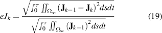
where  and
and  are the
  distributions for the iteration
  and
and  , respectively. If the error
  is smaller than a user-predefined criterion
  , then the process is completed. A detailed description of the H iterative multi-scale strategy can be consulted in [49].
The H iterative multi-scale model uses the same set of analyzed tapes used by the H multi-scale model, therefore figure 11(a) also represents the geometry of coil submodel of the H iterative multi-scale model.
The iterative multi-scale strategy requires the interpolation of the  distributions, the linear and the inverse cumulative density function (ICDF) interpolation methods were used. The ICDF interpolation method [56] was adapted to interpolate
  distributions in [49]. This method produces more realistic current density distributions, avoiding some issues produced by the conventional linear interpolation. The implementation of ICDF interpolation, as presented in [49], requires the computation of integrals, derivatives and inverse functions. In the H iterative multi-scale model, this method is implemented in a MATLAB script. The following simultaneous multi-scale models presented below were implemented in a single COMSOL model, and for convenience just the simpler linear interpolation was used. This is not a major drawback because the ICDF interpolation makes only a marginal contribution to the accuracy of the model [49].
4.5. Simultaneous multi-scaling
As described above, the H multi-scale and the H iterative multi-scale strategies use two different submodels. The computation of the  distributions in the analyzed tapes using the single-tape submodel can only be performed after the computation of the background magnetic field using the coil submodel. Therefore, the computation of the
  distributions and the background field is not carried out simultaneously.
In this section, a new strategy called simultaneous multi-scale is proposed. The simultaneous multi-scale strategy allows simultaneously solving the  distribution and the background magnetic field. The strategy relies on the possibility to include an additional contribution to the Ampère's law (equation (1)). This summand allows imposing an external current density
  in the superconducting subdomains
  of the non-analyzed tapes, as follows

Faraday's law (equation (2)) and the constitutive relations of the materials are used to derive the governing equation of the H formulation, which is expressed as
The external  in the superconducting subdomains
  of the analyzed tapes and in the surrounding medium subdomain
  is zero. The external
  in the superconducting subdomains
  of the non-analyzed tapes is approximated by interpolating the
  distributions of the analyzed tapes.
The resistivity in the superconducting subdomains  of the analyzed tapes is defined by equations (10) and (11). The resistivity of the superconducting subdomains
  of the non-analyzed tapes is considered to be the resistivity of the surrounding medium,
  . This value is orders of magnitude larger than the resistivity of the superconducting subdomains, therefore the induced current density in the non-analyzed tapes has a negligible impact when compared with the external
  .
.
The H simultaneous multi-scale model of the case study considers the same set of 30 analyzed tapes of the H multi-scale model. The non-analyzed tapes in the H simultaneous multi-scale model preserve their original geometry. Hence, figure 11(a) also represents the geometry of the H simultaneous multi-scale model. It is possible to reduce the number of degrees of freedom (DOF) and the computational burden of the H simultaneous multi-scale model by means of the homogenization or the densification of the non-analyzed tapes. Therefore, two additional models are presented here: the H simultaneous multi-scale homogenous model and the H simultaneous multi-scale densified model.
In the H simultaneous multi-scale homogenous and H simultaneous multi-scale densified models not all the non-analyzed tapes are homogenized or densified. The non-analyzed tapes adjacent to the analyzed tapes keep their original shape. These non-homogenous/non-analyzed or non-densified/non-analyzed tapes are used to move the distortions in the magnetic field produced by the homogeneous or densified tapes away from the analyzed tapes. The geometries of the three H simultaneous multi-scale models are presented in figure 11.
4.6. Results
To compare and validate the strategies described in this section, these models too were simulated for a sinusoidal transport current (11 A, 50 Hz). The results of the H homogenous, H densified, H multi-scale and H iterative multi-scale models are presented in figure 12. The results of the three H simultaneous multi-scale models are presented in figure 13. These figures have the format of figure 5. The first two columns show  and
and  , both at
  , the average losses are displayed in the third column, and the last column contains the quantitative data.
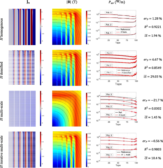
Figure 12. Results of H homogeneous, H densified, H multi-scale and H iterative multi-scale and models. The first and second columns show, respectively,  and
and  at the first negative peak of the transport current (
 ). The third column shows the average losses as a function of the tapes' number inside each pancake.
Download figure:
Standard image High-resolution image
Figure 13. Results of the H simultaneous multi-scale, H simultaneous multi-scale homogenous, and H simultaneous multi-scale densified models. The first two columns present the results at the first negative peak of the transport current ( ). The third column shows the average losses.
Download figure:
Standard image High-resolution imageThe first row in figure 12 shows the results of the H homogenous model. This model successfully reproduces the screening currents of the reference model. The  plot in this row shows how the individual tapes were replaced by the homogenous bulks. The
  distribution presents a smoother profile due to the homogenous current densities. The accurate estimation provided by this model is confirmed by the following values:
  and
and  . In this case the coefficient
  is computed using the rescaled current density (divided by
  ) and considering just the values at the positions of the original superconductor subdomains. The computation time required by the H homogenous model is 36 min 44 s (
 ).
).
The second row in figure 12 presents the results of the H densified model. Thicker lines are used to represent the densified tapes. In contrast to the homogenous case, here the  distribution has a jagged profile. This profile degrades the accuracy as can be observed in the values
  and
and  . For the purpose of computing
  , the
, the  distributions of the densified tapes are rescaled (divided by
  ) and the
  distributions in the removed tapes are approximated with linear interpolation. The computation time is reduced compared to the H full model, but this reduction is not as big as in the case of the H homogenous model, the normalized computation time is
  .
.
The results of the H multi-scale model are presented in the third row of figure 12. The predefined current density distribution  is uniform, as can be seen in the first entry of the third row. The uniform
  does not contain any screening current, then it is not a good approximation of the reference
  distribution. This fact is also reflected in the low coefficient
  . Consequently, the magnetic flux density and the losses exhibit noticeable errors, especially at the upper portion of the pancakes. The red circles in the plot of the losses indicate the position of the analyzed tapes, this is also the case of all the multi-scale models. The losses error is
  , the negative sign indicates that the losses are underestimated. The computation time is 27 min 30 s (
 ). This time is the summation of the time required to run the coil submodel one time (5 min) and the single-tape submodel 30 times, one for each analyzed tape (the average computation time of the single-tape submodel is 45 s).
The results of the H iterative multi-scale model are listed in the last row of figure 12. The convergence criterion is defined as  , this criterion is reached at the 7th iteration regardless of the interpolation method (linear or ICDF) used to approximate the
  distributions in the non-analyzed tapes. Figure 12 presents the results when the ICDF interpolation is used. The results when the linear interpolation is applied are visually indistinguishable from those obtained from the ICDF interpolation, then for clarity only the latter are shown. The error
  when linear interpolation is used is
  , when ICDF interpolation is used
  . The coefficient
  takes values 0.9796 and 0.9803, for the linear and ICDF interpolations, respectively. The accuracy is marginally better with the ICDF interpolation. The computation time is 3 h 21 min (
 ) with linear interpolation, and 3 h 17 min (
 ) with ICDF interpolation. These times are approximately seven times the computation time of the H multi-scale model.
The rows of figure 13 compiles the results of the H simultaneous multi-scale, H simultaneous multi-scale homogenous, and H simultaneous multi-scale densified models, respectively. The plots in the first column allow the observation of the different approaches in which the non-analyzed tapes are modeled: tapes with their original geometry, homogenous bulks or densified tapes. The  distribution of the H simultaneous multi-scale is visually indistinguishable from that of the reference model. Moreover, it is easy to find similarities between the distortions in the
  distributions of the H homogenous and H simultaneous multi-scale homogenous models, and between the distortions of the H densified and H simultaneous multi-scale densified models. The three models have acceptable and similar accuracies, as demonstrated by the
  values lower than
  , and the
  values greater than 0.98. The advantage of the homogenization and densification of the non-analyzed tapes is clearly observed in the computation times. The computation times of the H simultaneous multi-scale is 16 h 56 min (
 ). This computation time is approximately two times the computation time of the other two models.
5. T-A formulation strategies
5.1. Homogenization
The manner in which the homogenization is used in conjunction with the T-A formulation is depicted in figure 14. The magnetic vector potential  is defined all over the entire bounded universe. The stacks of 1D HTS layers are transformed into 2D bulks, and the potential
  is exclusively defined inside the bulk. For the purpose of computing
  , the influence of the component of
  parallel to the surface of the tapes is not considered, in figure 14 this parallel component is
  . Therefore, from equation (4), it follows that T has only one non-zero component (
 in the case of figure 14), which is defined by means of equation (5). Nevertheless, the parallel component
  influences the calculations by means of the definition of
  , see equation (11).

Figure 14.
T-A homogeneous strategy.  is defined in the entire bounded universe, and
  is exclusively defined inside the bulk. The boundary conditions
  and
and  are applied to the vertical edges of the bulk. The engineering current density
  is imposed into the A formulation.
Download figure:
Standard image High-resolution imageThe densely packed stack (homogenous bulk) must carry a transport current that is the summation of the transport current of the tapes making up the original stack. To impose such transport current, it is necessary to use the values  and
and  , defined in equation (6), as Dirichlet boundary conditions along the edges of the bulks perpendicular to the tapes. To compensate for the fact that the current density is computed inside the homogenous bulk, a new homogenized current density
  is defined as

where  is the ratio defined in equation (17).
  is imposed as a source into the A formulation, then equation (7) is transformed into,

For the purpose of computing T, the resistivity of the bulk subdomains is considered to be the resistivity of the superconducting material, defined by equations (10) and (11). The losses are computed by integrating the local losses along the lines parallel to the HTS layers at the center of each bulk's subset, then the losses along the rest of the tapes are approximated by interpolation. A more detailed description of the T-A homogenous strategy can be consulted in [50].
The T-A homogenous model of the case study, similarly to the H homogenous model, considers five bulks. Here, the integral constraints (one per bulk's subset) are not required to impose the transport currents. These subsets are used to define the distribution of the elements along the bulk's height. The mesh of the bulks in the T-A homogeneous model is structured and considers one element along the subsets thickness and 60 elements along the tapes' width. Figure 7 also represents the geometry of the T-A homogenous model.
5.2. Densification
The densification method can also be used in conjunction with the T-A formulation. Here too, the idea is to model the original stack by means of a smaller number of densified tapes.
In a T-A densified model the densified tapes are one-dimensional objects along which the  distributions are computed by means of the current density potential
  , and its only non-zero component
  , as given in equation (5). The resistivity of the HTS material is defined by means of equations (10) and (11). Unlike the H densified strategy, here the critical current density is not modified. In the T-A formulation, the surface current density
  is imposed into the A formulation, see equations (8) and (9). Thus, to take into account the densification of the tapes and to preserve the electromagnetic behavior of the original stack, the surface current density to be imposed is now scaled so that

where  is the number of tapes merged into a single densified tape.
Also the T-A densification process depicted in figure 8 involves two steps. The first step is to remove the tapes  1 and
1 and  . Second, the magnetic effect of tape
  is forced to be three times larger than the magnetic effect of the same tape in the T-A full model. The transport current in the densified tape remains the same as the transport current in the original tapes, see equation (6). The magnetic effect of the densified tapes is incremented by means of the parameter
  in equation (24). The losses can be calculated in the densified tapes, these losses are considered as the losses produced by the tapes of the original stack in the position of the densified tapes. The losses in the removed tapes are approximated by interpolation.
The T-A densified model of the case study considers the set of densified tapes of the H densified model, 31 densified tapes per pancake. Then, figure 9 also represents the geometry of the T-A densified model.
5.3. Simultaneous multi-scaling
The T-A simultaneous multi-scale strategy, as well as the H simultaneous multi-scale strategy, does not require two different submodels. The computation of the background magnetic field and the  distribution are carried out in a single model based on the T-A formulation.
In the T-A full models, the current vector potential  is defined over all the tapes. In the present approach,
  is defined only along the analyzed tapes. The
  distribution along the analyzed tape is obtained by calculating
  see equation (5). The
  distributions in the non-analyzed tapes are approximated by linear interpolation using the
  distributions of the analyzed tapes. The magnetic potential
  is defined over the entire bounded universe. The current density in both analyzed and non-analyzed tapes is multiplied by the thickness of the superconducting layer
  to obtain a surface current density
  to be imposed into the A formulation, see equations (8) and (9).
As it was the case with the H simultaneous multi-scale models, the DOF can be reduced by means of the homogenization or densification of the non-analyzed tapes. Therefore, three T-A simultaneous multi-scale models are presented. The difference between these models is the treatment of the non-analyzed tapes. The three models use the same set of six analyzed tapes per pancake used in the H multi-scale models. The first model, called T-A simultaneous multi-scale, considers the non-analyzed tapes with their original number and geometry.
As justified in [50], the T-A formulation uses first order elements to approximate  , and second order elements to approximate
  . If first order elements are used for both quantities, the computation time can be reduced [48], but this choice produces undesired spurious oscillations in the
  distributions [50]. To increase the computational efficiency without compromising the accuracy, the unit cells of the analyzed tapes and their adjacent non-analyzed tapes use second order elements to approximate
  , while first order elements are used to approximate
  throughout the rest of the system. Additionally, 30 elements are considered along most of the non-analyzed tapes, while 60 elements are considered in the analyzed tapes and their adjacent non-analyzed tapes. A more detailed description of the T-A simultaneous multi-scale strategy can be consulted in [50].
The other two T-A multi-scale models modify the geometric description of the pancakes by means of the homogenization or densification of the non-analyzed tapes. These models are called T-A simultaneous multi-scale homogenous and T-A simultaneous multi-scale densified models, respectively. As it was done in section 4.5, the non-analyzed tapes adjacent to the analyzed tapes keep their original geometry. These tapes with their original geometry are used to move the distortions in the magnetic field away from the analyzed tapes. The geometries of the T-A multi-scale models correspond to the geometries of the H multi-scale models, and are shown in figure 11.
5.4. Results
The T-A models were validated with the same operating conditions used in the previous sections. The results are compiled in figure 15, using the tabular format of figure 5.

Figure 15. Results of the T-A model. The  and
and  plots show the results at the first negative peak of the transport current (
 ). The third column shows the average losses. The three multi-scale models use the usual set of six analyzed tapes per pancake. The references results used to compute
  ,
,  and
and  are those of the reference model presented in section 3 and figure 5.
Download figure:
Standard image High-resolution imageThe first row in figure 15 shows the results of the T-A homogenous model. Due to the homogenization process, a smoother  distribution can be observed. In the loss plot of this row, the losses in the pancake 1 deviate from the reference results. The losses in the first pancake are two orders of magnitude lower than those of the pancake 5, therefore the deviation does not affect the global result. The total losses are slightly overestimated, the error is
  . The computation time required by the T-A homogenous model is 14 min 51 s (
 ).
).
The results of the T-A densified model are presented in the second row of figure 15. The densification process causes a more jagged  distribution. The coefficient
  demonstrates that, among the T-A models, the worst approximation of the current density is achieved by the T-A densified model. However, it remains an acceptable strategy for estimating the losses, as demonstrated by the value
  . In contrast to the H densified model, here the losses are slightly underestimated. The computation time of the T-A densified model is 61 min (
 ), approximately one third of the computation time of the T-A full model.
The last three rows contain the results of the T-A simultaneous multi-scale models. The  and
and  distributions calculated with the T-A simultaneous multi-scale model is indistinguishable from the distributions of the reference model presented in figure 5. The
  distributions of the T-A simultaneous multi-scale homogenous and densified models show the respective distortions produced by the homogenization and densification of the non-analyzed tapes. Accurate estimations are achieved with the three T-A simultaneous multi-scale models. In the three cases, the magnitude of the error
  is less than
  , and the coefficient
  is greater than
  . The computation time of the T-A simultaneous multi-scale model (
 ) is half that of the T-A full model (
 ). The densification of the non-analyzed tapes further reduces the computation time by 30 min (
 ). Conversely, the homogenization of the non-analyzed tapes produces a noticeable increment of the computation time (
 ).
).
6. Comparison
For ease of comparison; the error  , the coefficient
  , and the normalized computation time
  are brought together in table 3 to determine which model is the most efficient strategy. Additionally, the number of DOF of each model are presented. The first comparison, arising from table 3, is the comparison between the reference and the H full models. The reference model is the model with the largest numbers of DOF and the largest computation time. The reduction in the number of elements causes a reduction of the same order in the number of DOF. The speed up factor (
 ) due to the reduction of the number of elements is about 1.8.
Table 3. Models comparison.
| Model | Losses (W m−1) | Comp. time (h) | DOF | ||
|---|---|---|---|---|---|
| Reference | 127.24 | 31 h 32 min | 563 893 | ||
| Model |
 (%) (%) |

|
 (%) (%) | DOF | |
| H full | 1.62 | 0.9848 | 55.81 | 359 408 | |
| H homogenous | 1.28 | 0.9221 | 1.94 | 11 838 | |
| H densified | 6.67 | 0.8549 | 29.03 | 120 424 | |
| H multi-scale | −21.7 | 0.0302 | 1.45 | cs-112 752, st-709a | |
| H iterative multi-scale | −0.56 | 0.9803 | 10.41 | cs-112 752, st-709a | |
| H simultaneous multi-scale | 1.57 | 0.9833 | 53.70 | 359 408 | |
| H sim. multi-scale homogeneous | 0.72 | 0.9818 | 27.54 | 66 752 | |
| H sim. multi-scale densified | 0.99 | 0.9851 | 26.45 | 158 643 | |
| T-A full | 0.64 | 0.9922 | 10.25 | 548 624 | |
| T-A homogenous | 0.71 | 0.9214 | 0.78 | 20 612 | |
| T-A densified | −2.62 | 0.8854 | 3.22 | 103 638 | |
| T-A simultaneous multi-scale | 0.31 | 0.9913 | 5.06 | 114 582 | |
| T-A sim. multi-scale homogeneous | −0.25 | 0.9912 | 18.41 | 107 529 | |
| T-A sim. multi-scale densified | 0.61 | 0.9831 | 3.46 | 112 853 | |
a The abbreviation cs stands for the DOF of the coil submodel, and the abbreviation st stands for single-tape submodel.
The densification of the tapes in the H densified model allows reducing the DOF and the computation time, but this model has the second lowest accuracy with a coefficient  . The number of densified tapes in the densified model has to be larger than the number of analyzed tapes in the multi-scale models, otherwise the accuracy is drastically affected.
The model with the lowest number of DOF is the single-tape submodels of the H multi-scale and H iterative multi-scale models. The coil submodel has more DOF, and their computation is 5 min. However, the computation time of the H multi-scale model is mostly determined by the size of the single-tape submodel and the number of analyzed tapes. Despite the repeated use of the single-tape submodel, the H multi-scale model is the one with the lowest computation time among the models using the H formulation. However, the accuracy of the H multi-scale model is the lowest (
 ). The accuracy is improved by the iterative implementation of the multi-scale strategy; but the computation time increases. For the case study used here, the number of iterations is seven. Therefore, the computation time of the H iterative multi-scale model is approximately seven times that of the H multi-scale model.
The computation time of the H simultaneous multi-scale model is similar to that of the H full model; both models share the same variables, geometry, and number of DOF. The H simultaneous multi-scale model avoids the presence of the non-linear resistivity of the superconductor material in the non-analyzed tapes, as described in section 4.5. Nevertheless, this simplification in the non-analyzed tapes is not reflected in the computation time, likely due to the imposition of the interpolated  distributions and the interpolation process itself. The homogenization and densification of the non-analyzed tapes in the H simultaneous multi-scale homogeneous model reduces the number of DOF, with the larger reduction in the case of the homogenization. These reductions, even different, allow reducing the computation time roughly by a factor of two. The accuracy of the H simultaneous multi-scale models is similar for the three cases, with coefficients
  larger than 0.98, and errors
  lower than
  .
.
The T-A full model has more DOF than the H full model, this difference is mostly due to the use of second-order elements to approximate  in the T-A formulation. Despite the larger number of DOF, the T-A full model is approximately five times faster than the H full model. Both full models consider the same number of elements along the tapes' width, hence the reduction in the computation time is just influenced by the choice of the formulation.
Among the T-A models, the one with the lowest accuracy ( ) is the T-A densified model. This coefficient is similar to that of the H densified model, this similarity indicates that there is a systematic degradation in the accuracy due to the densification process. In both cases, the accuracy reduction results from the distortions in the magnetic field produced by the separation between densified tapes.
When going from the H full model to the H simultaneous multi-scale model, the number of DOF remains the same; conversely when going from the T-A full model to the T-A simultaneous multi-scale model the number of DOF is reduced. This reduction is possible because in the T-A simultaneous multi-scale model the vector potential  is not computed in the non-analyzed tapes, and the DOF associated with
  in the non-analyzed tapes are not required. The superiority of the T-A simultaneous multi-scale model over the H simultaneous multi-scale becomes clear when the computation times are compared. The T-A simultaneous multi-scale model is approximately ten times faster than the H simultaneous multi-scale model. At the same time, the T-A simultaneous multi-scale model is two times faster than T-A full model. The accuracy of the T-A simultaneous multi-scale model (
 ) is slightly better than the H simultaneous multi-scale model (
 ).
).
The speed of the T-A simultaneous multi-scale model can be boosted by means of either homogenous bulks or densified tapes to model the non-analyzed tapes. The accuracy of the three T-A simultaneous multi-scale models is similar, with coefficients  between 0.9831 and 0.9913. Indeed, the computation time is reduced in the T-A simultaneous multi-scale densified model, but in the T-A simultaneous multi-scale homogeneous model this time is more than three times the computation time of the T-A simultaneous multi-scale model.
Other than the single-tape submodels of the H multi-scale models, the models with the lowest number of DOF are the H and T-A homogenous models. When compared to their respective full models the speed up factors induced by the homogenization are 28.8 and 13.1, for the H and T-A homogenous models, respectively. At the same time, the T-A homogenous model (15 min) is approximately 2.5 times faster than the H homogenous model (37 min). The T-A homogenous model is the fastest one, because it benefits from the speed up factors offered by the T-A formulation and the homogenization. Nevertheless, the homogenization causes some distortions in the  distribution; the presence of such distortions is reflected in the reduction of the coefficients
  to around 0.92 for both homogeneous models.
The data compiled in table 3 is used to build the bubble chart presented in figure 16. The x-axis represents the absolute value losses error  , and the y-axis represents the normalized computation time
  , then the models with a bubble closer to the origin better fulfill the compromise between accuracy and computation time. The areas of the bubbles are proportional to the number of DOF. The H models are represented with solid bubbles, while the T-A models are represented with striped bubbles. In general, the striped bubbles (T-A models) are closer to the origin. Among the H models, those closer to the origin are the H homogenous and the H iterative multi-scale models. It is worth mentioning that the T-A homogeneous (striped black bubble), T-A simultaneous multi-scale (striped green bubble) and T-A simultaneous multi-scale densified (striped cyan bubble) models are within the first square of the grid, which means that
  and
and  are lower than 1% and 10%, respectively. With respect to the computation time, the largest numbers are those of the H full (solid blue bubble) and H simultaneous multi-scale (solid green bubble) models. The largest error
  is that of the H multi-scale model (solid orange bubble), this value is so large that the x-scale has a jump after 7%.

Figure 16. Bubble chart presenting the trade-off between accuracy and computation time. The bubbles closer to the origin are those of the models that better fulfill the compromise between accuracy and computation time. The areas of the bubbles are proportional to the number of DOF.
Download figure:
Standard image High-resolution image
The comparison of the different strategies was made with the same case study, when dealing with systems of different size the numbers may be slightly different, but the general conclusions are still applicable. The accuracies are not compromised by the size of the system, because they can be easily improved by increasing the number of bulk's subsets, densified or analyzed tapes. Moreover, the computation times and therefore the speed-up factors may experience larger variations. In some larger cases the memory requirements and the huge computation times prevent the implementation of full models. For instance, the 32 T all-superconducting magnet from the National High Magnetic Field Laboratory (NHMFL) in Tallahassee has an HTS insert made of more than 20 000 turns of REBCO tape [57–59]. It is reported in [60], that the T-A homogenous model of the 32 T magnet [61] is 396.2 times faster than the H iterative multi-scale model of the same magnet [62]. For the case study of this article the T-A homogenous model is 13.35 times faster than the H iterative multi-scale model.
7. User friendliness
One important aspect to consider when comparing the different strategies is the user friendliness, i.e. the ease with which the models can be built. However, it is not easy to quantify this aspect, because it widely depends on the expertise of the analyst. Additionally, each model has its own specificities, making it more difficult to compare them. As stated previously, all the models presented in this article were implemented in COMSOL Multiphysics. In general, the strategies described here allow analyzing systems made of stacks of HTS tapes. Therefore, it is mandatory for the analyst to master simple COMSOL features, e.g. copy, paste, move, built arrays and define selections. These COMSOL features allow not only building the geometry but also building the mesh in an efficient way.
The H multi-scale and H iterative multi-scale models are the most difficult to build, because they require building two submodels and implementing the communication between them. The communication and the iterative calling of the COMSOL submodels was implemented by means of MATLAB scripts. Extracting the background field at the correct boundaries of the analyzed tapes and interpolating the  distributions make these MATLAB scripts real clockwork mechanisms.
The reference and H full models are less difficult to build than the H iterative multi-scale model. Nevertheless, the imposition of the transport currents in each individual tape by means of integral constraints is a time consuming task. Fortunately, this task may be automated using tools like the COMSOL LiveLink for MATLAB. The T-A full model also requires the imposition of the transport currents in each tape. Nevertheless, this step does not require the definition of integral constraints, and the easier-to-handle Dirichlet boundary conditions at the edges of the tapes are used.
The simultaneous multi-scale models do not require two different submodels, and the imposition of the transport currents by means of integral constraints or Dirichlet boundary conditions is just necessary in the analyzed tapes. However, due to the interpolation of the  distributions, building the simultaneous multi-scale models is not easier than building the full models. The interpolation of the
  distributions requires using additional COMSOL features, e.g. extrusions, functions, variables and external current densities.
Without a doubt, the homogenous are the easiest-to-build models. First, the geometry of the stacks is simplified, and instead of all tapes it is just necessary to draw the bulks. Additionally, the imposition of the transport currents is easier. In the case of the H homogenous model, one integral constraint is necessary for each bulk's subset, then the number of constraints is lower than in the case of the H full model. In the case of the T-A homogeneous model the transport currents are imposed by means of Dirichlet boundary conditions along the edges of the bulks. The Dirichlet boundary conditions are easier-to-handle than the integral constraints; then the T-A homogeneous model is not only the fastest, but also the easiest-to-build model
8. Conclusions
It has been demonstrated that, in general, advanced methods, i.e. homogenization, densification and multi-scaling, allow quicker results without seriously compromising the accuracy. The only case in which the computation time is not reduced is the H simultaneous multi-scale. The only case in which the accuracy is not satisfactory (compared with the rest of the models presented here) is the H multi-scale. Accordingly, the models using an advanced method represent a good alternative to the full models, an alternative that is more significant in the cases where the size of the system complicates or makes the implementation of full models impossible.
As claimed in [45], the H formulation has a widespread popularity within the applied superconductivity community. However, the T-A formulation has proven to be more efficient to model systems made of HTS tapes. Accordingly, the strategies based on the T-A formulation have lower computation times than their H formulation counterparts. It is important to emphasize that the T-A homogenous model has the lowest computation time. Nevertheless, the T-A strategies inherit the limitations of the T-A formulation, i.e. they are intrinsically limited to cases where the 1D approximation of the superconducting layer is meaningful. On the contrary, the H strategies, except for the H homogenous strategy, are also suitable for the analysis of systems made of wires with different geometries, like MgB2 wires.
There may be cases of a sufficiently large system where the memory recourses of the available computer are surpassed, even for the homogenous models. The H iterative multi-scale models have the advantage that they can be used to analyze large-scale systems almost without size limit. The reason is that the number of DOF of the single-tape model remains constant independently of the size of the system. The coil submodel, being a magnetostatic model, requires a lesser amount of computational resources to be simulated, therefore it is possible to analyze considerably larger systems. Furthermore, the H iterative multi-scale models have the additional advantage that the simulation of the analyzed tapes by means of the single-tape submodel can by parallelized, further reducing the computation time.
Acknowledgments
This work was supported in part by the Programa de Maestría y Doctorado en Ingeniería of the Universidad National Autónoma de México (UNAM) and the Consejo Nacional de Ciencia y Tecnología (CONACYT) under CVU: 490544, and by DGAPA-UNAM grant, PAPIIT-2019 IN107119.