
Abstract
Streamer discharges occur in the early stages of electric breakdown of gases in lightning, as well as in plasma and high voltage technology. They are growing filaments characterized by a curved charge layer at their tip that enhances the electric field ahead of them. In this study, we analyze the effect of strong electron attachment on the propagation of positive streamers. Strong attachment occurs in insulating gases like sulphur hexafluoride (SF6) or in air at increased density. We use the classical fluid approximation with photo-ionization for streamers in ambient air, and we artificially increase the electron attachment rate where the field is below the breakdown value. This modification approximates air pressures above 1 bar at room temperature. We find that the streamer head can keep propagating even though the ionized channel loses its conductivity closely behind the head; hence, even if it is electrically isolated. We describe how, depending on the attachment rate, the streamer propagation in a constant electric field can be accelerating, uniformly translating, or stagnating.
Export citation and abstract BibTeX RIS

Original content from this work may be used under the terms of the Creative Commons Attribution 4.0 licence. Any further distribution of this work must maintain attribution to the author(s) and the title of the work, journal citation and DOI.
1. Introduction
Streamers [1–3] are fast-growing ionized filaments whose development is governed by the creation of a curved space charge layer around them and the self-enhancement of the electric field ahead of them. Streamers can be formed in gases [4] and in liquids [5] when the electric field locally exceeds the breakdown threshold even though the background electric field is below breakdown.
In nature, streamers occur as precursors of sparks and lightning leaders, and they are visible as sprites above thunderclouds. In plasma technology, streamers are used in various applications [6–10], for example, in plasma medicine [11–13], plasma-assisted combustion [14, 15], surface treatment, and thin film deposition [16].
Streamers occur with positive or negative polarity. Positive streamers have a positive net charge (i.e. positive space charge) at their tips, and they propagate in the same direction as the background electric field, which is against the direction of the electron drift. Negative streamers have a negative net charge (i.e. negative space charge) at their tips, and they propagate along the direction opposite of the background electric field, in the direction of the electron drift. In this paper, we focus on positive streamers, which form more easily than negative ones in air [17]. Since positive streamers propagate opposite the direction of the electron drift, they require a source of free electrons at their heads for propagation. In air, photoionization is the most important source of these electrons [4, 18].
As electrons enter the region where the electric field is above the breakdown value, referred to as the ionization zone, they multiply due to the electron-impact ionization reactions dominant in this region. However, in the interior region of the streamer where the electric field is below breakdown, electrons are lost due to attachment to electronegative molecules.
Attachment reactions are prevalent, in particular, in gases such as sulphur hexafluoride (SF6), which are used in high voltage equipment such as circuit breakers [19, 20]. In air, the attachment processes involve dissociative and three-body reactions with oxygen molecules. Like the rate of impact ionization and many other reaction rates in streamers, the dissociative attachment reaction rate increases linearly with the gas density. However, the three-body attachment reaction rate increases quadratically with gas density, and thus, its importance increases with it.
In this paper, our goal is to understand the effect of the electron attachment rate on the dynamics of positive streamers. In particular, we look at whether streamers can continue to propagate if the electrons in the channel get attached rapidly. To investigate this, we perform axisymmetric simulations of positive streamers in air at standard temperature and pressure with normal and modified attachment rates. In the latter cases, we systematically enhance the attachment rate in regions where the electric field is below the breakdown value, and we keep it unchanged in the high-field regions. This way, we focus only on the effect of the attachment rate on the streamer dynamics while we keep other parameters such as gas composition, impact ionization rate, and photoionization fixed. The details of this modification are given in section 2.2.
The structure of the paper is as follows. The discharge model and simulation conditions are presented in section 2, where the model equations along with the transport parameters and reaction rates are described in section 2.1, the computational domain and boundary conditions are supplied in section 2.3, and the initial conditions are given in section 2.4. The results are presented in section 3, where in section 3.1.2, we show that a streamer can keep propagating while the streamer head is electrically isolated from streamer body and electrode due to significant electron attachment behind the streamer head. In section 3.2, we discuss three modes of streamer propagation: accelerating, uniformly translating, and stagnating. Finally, in the concluding section 4, we summarize our results in section 4.1, and we relate our results on electrically isolated propagating streamer heads to concepts by other authors in section 4.2.
2. Discharge model
2.1. Model equations, transport parameters, and reaction rates
We used a drift–diffusion-reaction type fluid model to simulate positive streamers in artificial air, composed of 80% nitrogen and 20% oxygen, at standard temperature and pressure. Twelve reactions, listed in table 1, were considered: electron impact ionization (k1, k2), electron attachment (k3, k4), electron detachment (k5, k6), ion conversion (k7–k11), and electron–ion recombination (k12). The temporal evolution of the electron density (ne) is given by the continuity equation

where E is the electric field, μe is the electron mobility, De is the electron diffusion coefficient, Si is the electron impact ionization source term, Sη is the electron attachment source term, Sph is the non-local photoionization source term, and Sion contains all electron detachment reactions from the ions minus the electron–ion recombination reaction.
Table 1. Reactions included in the model, with reaction rate coefficients and references. M is any molecule, either O2 or N2. Te in reaction number 12 depends on E/N through the mean electron energy  as
as  [24], and
  is calculated with Bolsig+.
| Reaction No. | Reaction | Reaction rate coefficient | Reference |
|---|---|---|---|
| 1 |

|

| [21] |
| 2 |

|

| [21] |
| 3 |
|

| [21] |
| 4 | e + O2 → O + O− |

| [21] |
| 5 |
|
 exp exp 
| [22] |
| 6 | N2 + O−→e + N2O |
 exp exp 
| [22] |
| 7 |

|
 exp exp 
| [22] |
| 8 |
|
 exp exp 
| [22] |
| 9 |
| k9 = 5.0 × 10−41 m6 s−1 | [23] |
| 10 |
| k10 = 2.50 × 10⁻¹⁶ m3 s−1 | [23] |
| 11 |
| k11 = 2.40 × 10−42 m6 s−1 | [23] |
| 12 |

|

| [24] |
The impact ionization source term Si, the electron attachment source term Sη , and the photoionization source term Sph contain reactions of electrons with neutral molecules. These are the relevant plasma-chemical reactions in the ionization zone ahead of the streamer. They are calculated using the rate coefficients given in table 1:


Note that we do not include the three-body attachment reaction,  , in our model because its reactions rates are about three orders of magnitude smaller than k3 [24].
Si and Sη are linear in the electron density ne. As the degree of ionization at standard pressure and temperature and below is small within a streamer, the densities of neutral molecules [O2] and [N2] can be assumed to be constant. Therefore the impact ionization and attachment reactions can be written as the product of the electron flux μe Ene and the coefficients α and η respectively [3]. The effective ionization source term can then be defined as

The sign of αeff determines whether the local electron density increases or decreases in the streamer ionization front.
The photoionization source term Sph contributes only a small correction to the local reaction rates. However, it is very important due to its nonlocal nature, which allows for the liberation of electrons in the non-ionized region. It is given by

where  is the source of ionizing photons, f(r) is the absorption function, and 4π|r − r'|2 is a geometric factor. We employed the commonly used Zheleznyak's model [25], where
  is proportional to the electron impact ionization source term (Si)

Here p is the actual gas pressure, pq = 40 mbar is a gas-specific quenching pressure, and ξ is a proportionality factor that was set to ξ = 0.075. We approximated the integral in equation (5) using a set of Helmholtz differential equations [26, 27] with Bourdon's three-term parameters [27]. In addition to the original papers [26, 27], the reader is also referred to the appendix of [28] for more details.
In the ionized region inside the streamer, reactions involving ions are significant as well. The relevant terms affecting the electron density are

where [M] is the density of all neutral molecules: [M] = [N2] + [O2].
Other species Zi in our model are ionized or non-ionized molecules or atoms. According to table 1, these are  ,
,  ,
,  ,
,  , O−,
, O−,  ,
,  , and the neutrals O and N2O. Their densities are also calculated from a continuity equation

where si = ±1 is the sign of the electric charge of species i and μi is the ion mobility. The neutral species are treated as immobile. The drift of ions is neglected in most sections of the paper as their mobility is much smaller than that of electrons, but in section 3.5, we include the ion drift and discuss its effect on the previous results. All ion mobilities are assumed to be 2.2 × 10⁻⁴ m2 V−1 s−1 [29] in that set of simulations. As  , O, and N2O do not drive further reactions in our model, their densities do not need to be calculated in practice, except to account for the contribution of the
  ion to the space charge density.
The electric potential and the electric field are calculated as

where  0 is the vacuum permittivity,
  is the space charge density, e is the elementary charge, and ni is the density of all positive ions minus the density of all negative ions.
Most reaction rate coefficients in table 1 are a function of the reduced electric field E/N. Electron-neutral scattering cross sections for nitrogen and oxygen are taken from the Phelps database [21]. Bolsig+ [30] (version 03/2016 for Linux), an electron Boltzmann equation solver, was used to calculate the mean electron energy, transport coefficients μe and De, and the reaction rates for electron impact ionization and electron attachment (i.e. k1, k2, k3, and k4). Bolsig+ solved the Boltzmann equation under the assumption that the electron density grows exponentially in space without time dependence.
2.2. Modification of effective ionization coefficient
To identify the effect of strong attachment in regions below the breakdown field, the effective ionization coefficient was modified in such a way that the attachment rate in high electric field regions is unchanged and it is only enhanced in regions below the electric breakdown value. The photoionization rate is made unaffected by the changes in the coefficients.
This is accomplished in two steps. First, the effective ionization coefficient was multiplied by a factor m below the electric breakdown field Ec, which is about 28 kV cm−1 in our case.

This translates to multiplying reaction rate coefficients k1, k2, k3, and k4 with the factor m when used in regions below the breakdown field. Above the breakdown field, the effective ionization coefficient is unchanged. Figure 1 shows the reduced effective ionization coefficient αm /N as a function of the reduced electric field strength E/N for different values of m. These so-called reduced quantities are scaled with the gas density N. The reduced effective ionization coefficient for air at 26 bar is included for comparison, and we see that its values match the m = 26 case for reduced electric fields below 30 Td, where three body attachment is dominating. As we describe later in section 3, the reduced electric fields inside streamer channels are found to be below 30 Td. Furthermore, the attachment rate in the m = 37 case, which has the highest attachment rate in this study, is still about one order of magnitude smaller than the respective rate in SF6 at standard temperature and pressure [21, 31].

Figure 1. Reduced effective ionization coefficients αm /N from equation (10) as a function of the reduced electric field E/N for the indicated values of m and the reduced effective ionization coefficient for air at 26 bar.
Download figure:
Standard image High-resolution imageSecond, the photoionization source term (6) was set to continue to use the unmodified ionization coefficient α.
2.3. Computational domain, electric field, and boundary conditions
The model is implemented in afivo-streamer [32, 33], which employs geometric multigrid techniques to solve Poisson's equation and OpenMP parallelism. We simulate cylindrically symmetric positive streamers in a volume spanned by radius r and axis z. The domain has a length of 50 mm and a radius of 50 mm. Adaptive mesh refinement is employed with the grid set to have a minimum size of 2 μm. The refinement and derefinement criteria are based on the local electric field value as in [32] with an additional criterion based on the charge density: refine if α(1.2 × E)Δx > 0.5 and derefine if  and
and  , where α(E) is the field-dependent ionization coefficient, E is the electric field strength, and Δx is the grid spacing. We apply a homogeneous background electric field by fixing the electric potential at z = 0 mm and z = 50 mm. Neumann zero boundary conditions are applied to the electric potential at r = 0 mm and r = 50 mm, and to the electron density at all boundaries. The electric field points in
  direction with a magnitude of 15 kV cm−1, which is about half of the breakdown field. No background ionization is incorporated in the domain.
2.4. Initial conditions
To initiate a positive streamer, we placed two neutrally charged cylindrical seeds on the axis of symmetry. The first seed serves as the initiation point of the streamer. It is 1 mm long with 2.25 × 10²⁰ m−3 electrons and positive ions and has a width of 0.25 mm. It extends from z = 50 mm to 49 mm. The second seed supplies additional electrons during initiation until photoionization provides sufficient electrons for continued streamer propagation. This seed is 2 mm long with 1.0 × 10¹⁷ m−3 electrons and positive ions and has a width of 0.2 mm. It extends from z = 49 mm to 47 mm. The seeds decay with a Gaussian profile along the r-axis throughout their length and radially decay with a Gaussian profile in all directions at the caps.
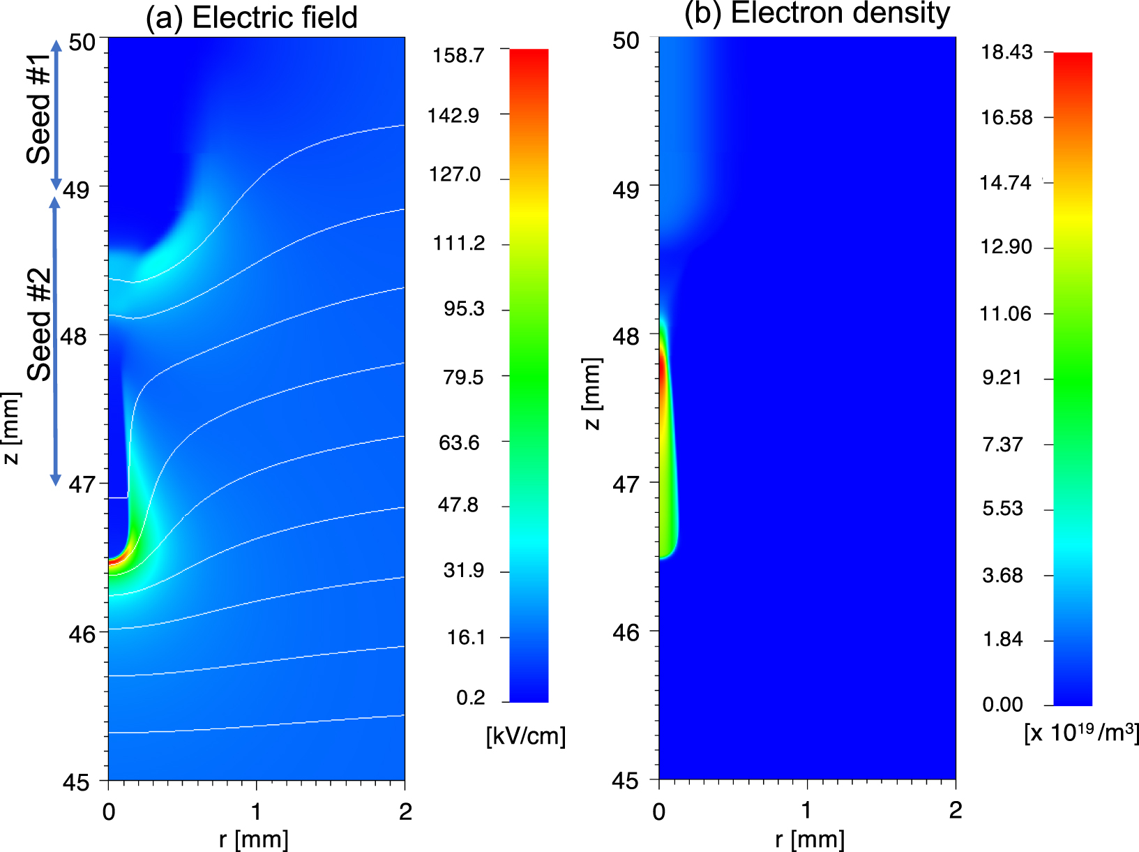
For air, which is the case of m = 1 in equation (10), a streamer initiates in such setup. However, for strongly enhanced attachment conditions with large values of m, a streamer does not successfully initiate. Therefore, we first ran our simulation with the normal attachment rate m = 1 for 20 ns to get a streamer and then take this stage, that is illustrated in figure 2, as the initial condition for all runs with values of m from 1 up to 37. At this stage, a streamer has clearly formed and grown to a length of about 3.53 mm and a radius of 153 μm.
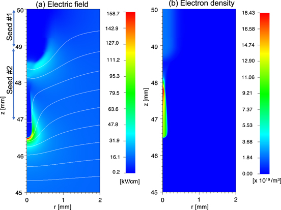
Figure 2. The initial condition at t = 0 ns for all streamer simulations presented in this paper, in radial coordinates (r, z): (a) electric field strength |E| (color-coded) with white equipotential lines, (b) electron number density. The streamer has initiated from the seeds at time t = −20 ns, and it has propagated to a length of about 3.53 mm at time t = 0 ns with m = 1. Note that the computation domain extends from 0 to 50 mm both in r and in z directions; however, in this figure only a part of the domain is shown.
Download figure:
Standard image High-resolution image3. Streamer evolution for different values of m
3.1. Two examples: m = 1 and m = 26
Figures 3 and 4 show the evolution of the streamer with m = 1 on the left hand side and the streamer with m = 26 on the right hand side. For m = 26, electron attachment is strongly enhanced when the electric field is below the breakdown value, while it is the same as in air when the field is above breakdown. The background field is 15 kV cm−1, which is about half of the breakdown field. The evolution of the m = 1 streamer is shown in time steps of 15 ns, and the evolution of the m = 26 streamer is shown in time steps of 30 ns. The m = 1 streamer propagates over a length of 30.4 mm within 45 ns, and the m = 26 streamer propagates over a length of 22.8 mm within 90 ns.
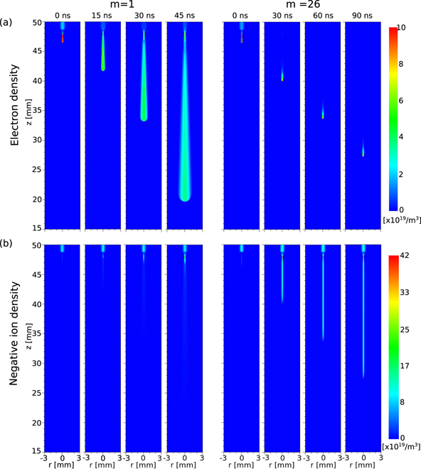
Figure 3. Streamer evolution in air with different electron attachment rates: normal attachment (m = 1) at times 0, 15, 30, and 45 ns on the left, and strong attachment rates (m = 26) at times 0, 30, 60, and 90 ns on the right. The background electric field is 15 kV cm−1. Shown are the electron density and the number density of negative ions (i.e. ![$\left[{\mathrm{O}}^{-}\right]+\left[{\mathrm{O}}_{2}^{-}\right]+\left[{\mathrm{O}}_{3}^{-}\right]$](https://content.cld.iop.org/journals/0963-0252/30/2/025006/revision6/psstabdaa3ieqn42.gif) ). Figure 4 contains the space charge densities and the electric fields for the same cases.
). Figure 4 contains the space charge densities and the electric fields for the same cases.
Download figure:
Standard image High-resolution image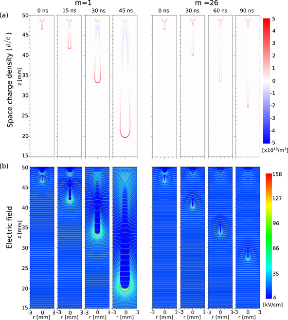
Figure 4. The same simulations as shown in figure 3, but here the space charge density ρ/e is plotted in the upper row with the electric field (color-coded) with equipotential lines (white) in the lower row.
Download figure:
Standard image High-resolution imageThe panels in figures 3 and 4 show the electron number density ne, the number density of all negative ions ![$\left[{\mathrm{O}}^{-}\right]+\left[{\mathrm{O}}_{2}^{-}\right]+\left[{\mathrm{O}}_{3}^{-}\right]$](https://content.cld.iop.org/journals/0963-0252/30/2/025006/revision6/psstabdaa3ieqn43.gif) , the space charge density ρ/e, and the electric field strength E = |E| with white equipotential lines ϕ. Within each row, the same color coding is used for the respective densities and the field strength. The figures zoom into the region r ⩽ 3 mm and 15 mm ⩽ z ⩽ 50 mm. The overall simulation volume extends to 50 mm in the r direction and 50 mm in the z direction.
, the space charge density ρ/e, and the electric field strength E = |E| with white equipotential lines ϕ. Within each row, the same color coding is used for the respective densities and the field strength. The figures zoom into the region r ⩽ 3 mm and 15 mm ⩽ z ⩽ 50 mm. The overall simulation volume extends to 50 mm in the r direction and 50 mm in the z direction.
3.1.1. m = 1
The streamer with the normal attachment rate, shown on the left hand side of figures 3 and 4, presents the familiar phenomenology: it forms an elongated ionized channel that largely suppresses the electric field in the channel interior and enhances it ahead of the streamer tip. The electric conductivity of the streamer body is due to the density ne of free electrons that drift in the local electric field. At the edge of the ionized region, the electric field changes strongly across the thin space charge layer; it is formed by the surplus or lack of free electrons relative to the density of positive ions. Within the strong external electric field of more than half of the breakdown value, the streamer radius grows in time and so does its velocity. Because the streamer head gets wider, more positive electric charge is required at its head. As charge is conserved, the negative charge moves backward, as can be seen in both the equipotential lines and the space charge density ρ/e. No considerable density of negative ions is formed in the streamer interior.
3.1.2. m = 26
The streamer with strongly enhanced attachment rate, shown on the right hand side of figures 3 and 4, has a very different behaviour even though the external field is the same and the plasma reactions are only changed in the region below the breakdown field. The streamer head propagates with a nearly constant and small radius and velocity. The density ne of free electrons that is created in the ionization front rapidly disappears behind the streamer head due to fast attachment, and it leaves a density of negative ions behind. A thin layer of positive charge surrounds the streamer head, but as the streamer propagates, only a faint negative charge appears at its back end that does not change the electric field in a significant manner. The streamer tip rather propagates in a solitary manner, and the electric field behind it returns to the background value, as can be read particularly clearly from the straight and parallel equipotential lines at some distance behind the streamer head.
Surprisingly, this electrically isolated streamer head keeps propagating essentially without changing its shape and without destabilizing. Thus, it behaves as a coherent structure, i.e., as a nonlinearly stabilized structure like a soliton.
3.2. Temporal evolution of maximal field, velocity, and radius
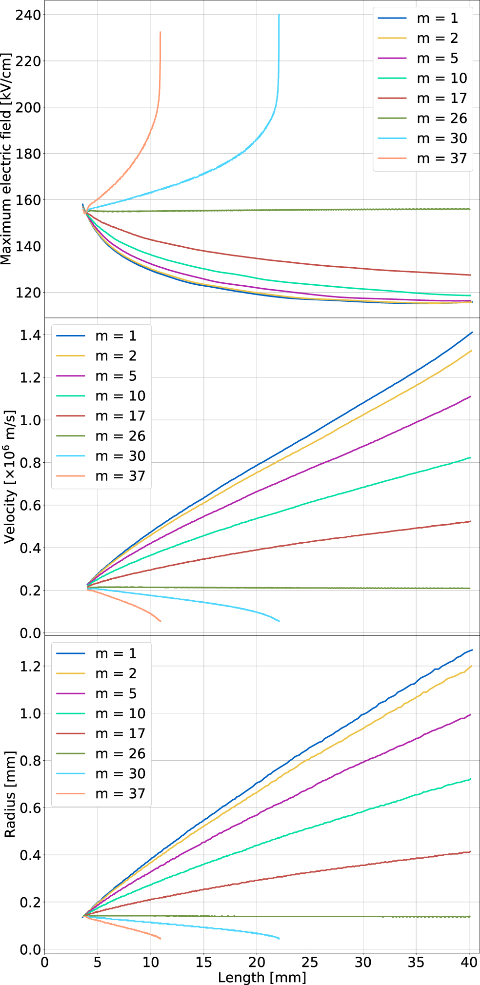
In figure 5, the maximal electric field Emax, streamer velocity v, and streamer radius R for different values of m are plotted as a function of streamer length L. The plot finishes at a length of 40 mm, while the electrode is at z = 50 mm. Hence, effects of electrode proximity are not shown. The streamer length is defined as 50 mm − zmax, where zmax is the location of the maximum electric field. As earlier in [28], the radius is measured as the location where the radial component Er of the electric field is maximal.

Figure 5. Maximal electric field (upper panel), streamer velocity (middle panel), and streamer radius (lower panel) as a function of streamer length L for different attachment rates m.
Download figure:
Standard image High-resolution imageThree different cases of streamer growth can be distinguished in figure 5:
- Accelerating streamers. For the case of artificial air (m = 1) as shown in figures 3 and 4, the streamer radius R increases with streamer length L from 0.146 to 1.00 mm and the streamer velocity v from 2.20 × 10⁵ m s−1 to 1.12 × 10⁶ m s−1, while the maximal electric field Emax at the streamer head decreases slightly from 158 kV cm−1 to 116 kV cm−1. The same tendency of increasing velocity and radius and decreasing maximal field as a function of streamer length is seen for all values of the attachment parameter m up to 26, though the rates of increase or decrease diminish with growing m.
- Uniformly translating streamers. The case of m = 26, that is also displayed in figures 3 and 4, is a limiting case: radius, velocity, and maximal field stay approximately constant while the streamer propagates. It is remarkable that this streamer head is dynamically stable, and that the motion is really a uniform translation where the background field is restored after the streamer head has passed and the nonconducting state is re-established.
- Decelerating and stagnating streamers. For m > 26, radius and velocity decrease with growing streamer length while the maximal electric field at the streamer tip grows very rapidly. In fact, the simulation stops, because the increasing electric field requires a too small numerical time step. Due to the CFL condition [33], the numerical time step has gone down to less than 10−14 s from 10−12 s with the maximal electric field suddenly reaching to values greater than 300 kV cm−1 in a limited region ahead of the streamer. From an investigation on negative streamers in [34], the local field approximation was found to no longer be valid at electric field values above 200 kV cm−1 at 1 bar, and this limit is greatly exceeded by our stagnating streamers before the simulations stop.
The way how the positive streamers for m > 26 decelerate, and eventually stop, is reminiscent of earlier observations of stagnating and 'dying' positive streamers [35, 36].
3.3. The front structure of streamers at 30mm length
Now, streamers of 30 mm length for different values of m are analyzed in more detail; more precisely, streamers that have propagated from z = 46.5 mm up to z = 20 mm. This occurs after a time of 44.75 ns for m = 1, after 87.25 ns for m = 17, and after 125 ns for m = 26. The cases of m = 30 and 37 are excluded, as these streamers do not reach this length.
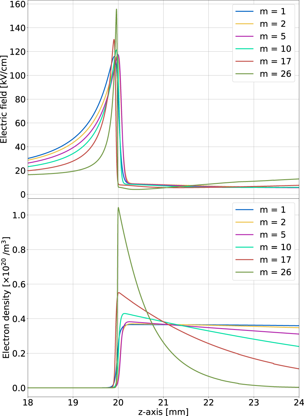
Figure 6 zooms into the region 18 mm ⩽ z ⩽ 24 mm, which is around the streamer head. It shows the electric field and electron density on the streamer axis for different values of m.
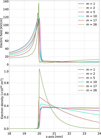
Figure 6. Zoom into the region around the streamer head when the streamers have reached a length of 30 mm. Shown are electric field (upper panel) and electron density (lower panel) on the streamer for different m values.
Download figure:
Standard image High-resolution imageThe electric field in the streamer front shows the familiar structure: the thin and weakly curved space charge layer at z = 20 mm (see figure 4) causes the field to jump from a highly enhanced value to a quite low one. Behind the space charge layer in the streamer interior (i.e. for larger z), the electric field is largely screened. The decay length of the electric field ahead of the space charge layer (i.e. for smaller z) is determined by the radius of curvature of the space charge layer. The maximum of the field is determined dynamically. It occurs to be higher for the slower and thinner streamers with higher m values.
The electron density is shown in the lower panel of figure 6 on a linear scale in the streamer head region. Where the electric field is maximal, the electron density is growing rapidly, almost discontinuously, in particular, for large m. The second panel of figure 7 shows the electron density on a logarithmic scale over a wider spatial range for m = 1, 17, and 26. Ahead of the front in the range of z < 17 mm, the electron density grows exponentially in space towards the front region, like exp [z/ℓ], with the same length scale ℓ = 1.1 mm, according to a fit in the range of z = 4 to 15 mm, for all three values of m. An analytical estimate shows that this length scale ℓ should be set by the largest photon absorption length in the photoionization model, and this length is indeed 1.2 mm [27, 28]). In the high field region at z ≈ 20 mm, the electron density increases steeply as in the linear plot of figure 6.
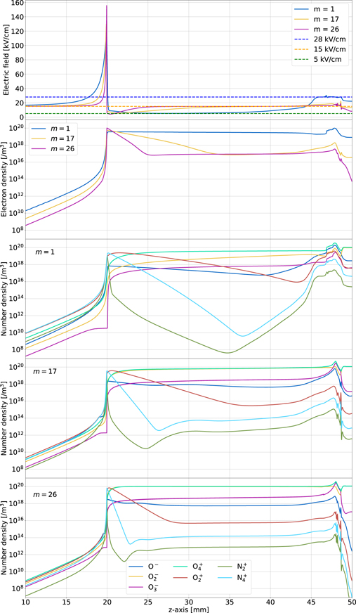
Figure 7. Electric field profile E (first panel), number densities of electron ne (second panel) and all ion species for different attachment rates (m = 1 on third panel, m = 17 on fourth panel, and m = 26 on fifth panel) on the streamer axis. Streamers of the same length are shown. The first panel also contains dashed lines for the breakdown field 28 kV cm−1, the background field 15 kV cm−1, and the field 5 kV cm−1 for reference. Legend on the fifth panel applies for the third and fourth panel as well.
Download figure:
Standard image High-resolution imageBehind the ionization region, the electron density is nearly constant for m close to 1, but it decreases for larger m with growing distance behind the front. For m = 17 and m = 26, it saturates to about 1017 m−3 at z > 33 mm and z > 25 mm respectively, which is the result of attachment and detachment reactions compensating each other. By inspecting the density of the ionic species in the streamer channel for the three cases shown in the third, fourth, and fifth panels of figure 7, we observe that the densities of  ,
,  , and
, and  differ significantly in m = 1, 17, and 26, whereas the densities of the other ionic species are quite similar. For m = 17 and m = 26, the density of ionic species also approach an identical constant value for both cases.
Surprisingly, the maximum value of the electron density generated in the ionization front is highest for the largest m, i.e. when the electron attachment rate in the region below breakdown is highest. Common estimates relate the maximal electron density behind the front to the maximal electric field at the front [34, 37, 38] though this relation somewhat deviates from numerical observations for positive streamers with photoionization [39], as discussed in section 3.4 of [3]. The present observation confirms that a higher maximal field creates a higher electron density behind the ionization front.
3.4. Charged species in 30mm long streamer channels
Figure 7 shows the electric field, electron density, and ion species on the streamer axis throughout the whole ionized region. Here, the streamer heads have arrived at z = 20 mm as before.
The upper plot shows the electric field on axis, and three constant values are inserted for reference: the breakdown field of 28 kV cm−1 (where αeff = 0), the applied background field of 15 kV cm−1, and the field of 5 kV cm−1 that is frequently observed in the interior of single positive streamers in air and interpreted as the so-called stability field. Far ahead of the streamers at z → 0, the electric field essentially has the background value, and then it increases strongly towards the streamer head, as described above. Behind the ionization front in the streamer interior, the electric field approaches 5 kV cm−1 for m = 1, while it approaches the background field of 15 kV cm−1 in the cases of m = 17 and 26. The axis range of 45 mm < z < 50 mm shows remainders of the initiation process and is not discussed further.
The different interior fields of 5 or 15 kV cm−1 are related to the different interior conductivities of the streamers. While for m = 1, there is a sufficient electron density to screen the electric field from the streamer channel, this is not the case for the middle and back regions of the streamers with m = 17 or 26 as we will discuss now.
The simulation results for electron attachment and ion conversion are shown in the lower three panels of figure 7. The reactions listed in table 1 involve electrons, neutrals, the positive ions  ,
,  ,
,  ,
,  , and the negative ions O−,
  ,
,  . As described in [23], all positive ions in air rapidly convert to
  . This statement is confirmed by the present simulations, where the densities of the other positive ions quickly decrease behind the ionization front.
For m = 1, the electrons created in the ionization front attach to oxygen mainly through three-body attachment, hence the  density increases behind the moving front in about the same manner as the electron density decreases. Dissociative attachment creating O− has no substantial contribution at standard temperature and pressure. As
  is produced in collisions of O2 with O−, its concentration stays low as well. It is quite a stable ion in air. There is a rapid trail of positive ion conversion within the streamer head, from
  to
to  to
to  . This is followed by the fast conversion of
  into
into  in the streamer channel.
For m = 17 and 26, the ionization and attachment reaction rates k1 to k4 are enhanced by a factor m in the region below the breakdown field. This concerns the complete streamer channel. Accordingly, the electron density decreases rapidly behind the ionization front, while the  density increases in about the same manner as the electron density decreases. For both values of m, an electrically neutral streamer channel is formed, consisting mainly of
  and
and  ions while all other ion densities are at least an order of magnitude smaller. Note that in figure 7, the yellow line that represents
  mostly coincides with the green line that represents
  for m = 17 and 26. As ion mobility is much smaller than electron mobility and neglected in the present model, this streamer channel cannot screen the electric field anymore and the field returns to the background value.
3.5. Electronic and ionic currents
Since electrons are quickly attaching and disappearing behind the streamer head for large values of m, the electric current due to the electrons is significantly decreasing along the streamer channel. Thus, ionic conductivity could possibly become relevant, and we investigate that here. We performed streamer simulations which included ion motion through the drift term in equation (8) with the finite ion mobility given in section 2.1.
The electronic conductivity was calculated with σe = ene
μe and ![${\sigma }_{\mathrm{i}}={\sum }_{i}\;e\left[{Z}_{i}\right]{\mu }_{i}$](https://content.cld.iop.org/journals/0963-0252/30/2/025006/revision6/psstabdaa3ieqn66.gif) was used for calculations of the ionic conductivity. From the conductivities, the current densities je and ji, for the electrons and the ions respectively, were calculated using je = σe
E and ji = σi
E. Figure 8 presents the electronic and ionic current densities on the streamer axis for cases m = 1, 17, and 26 when the heads have arrived at z = 20 mm as in the previous section.
was used for calculations of the ionic conductivity. From the conductivities, the current densities je and ji, for the electrons and the ions respectively, were calculated using je = σe
E and ji = σi
E. Figure 8 presents the electronic and ionic current densities on the streamer axis for cases m = 1, 17, and 26 when the heads have arrived at z = 20 mm as in the previous section.

Figure 8. Current density profiles for different attachment rates (m = 1, m = 17, and m = 26) on the streamer axis. Electronic current densities are shown with solid lines and ionic current densities with broken lines. Streamers of the same length are featured.
Download figure:
Standard image High-resolution image
For m = 1, the electronic current density is nearly 3 orders of magnitude higher than the ionic current density, rendering the effect of the ions to the total current negligible. For m = 17 and m = 26, at about z = 34 mm and 26 mm behind the ionization front respectively, the ionic current density starts to get larger than the electronic current density. This ionic current density is of the order of 1 kA m−2 for all values of m considered. Here, the densities of  and
and  are dominating in the increased attachment cases. Due to approximate charge neutrality in the streamer channel, the electric currents of positive and negative ions contribute about equally. The ionic current densities do not have a significant effect on the streamer behavior.
4. Conclusions
4.1. Summary
We have simulated and analyzed single positive streamers with photoionization in a constant electric field below the breakdown value. To study systematically the effect of electron attachment and of the subsequent loss of channel conductivity on the streamer dynamics, we performed simulations in artificial air (N2:O2 = 80:20) at standard temperature and pressure, and then we modified the effective ionization coefficient such that electron attachment is increased in the region below breakdown, while we kept all other parameters the same. Our main conclusions are:
- (a)A streamer head can keep propagating even if the ionized channel behind it loses its conductivity due to rapid electron attachment.
- (b)Depending on parameters, the streamer can be accelerating or decelerating. Between these parameter regimes, the streamer can propagate uniformly, i.e. with unchanged velocity and spatial structure. In this case, the electrically isolated streamer head carries a fixed amount of positive electric charge, and the electric field behind it returns to its background value.
- (c)It is remarkable that this uniform translation is dynamically stable, at least for the duration of our simulations. This illustrates that the streamer head is a coherent structure like a solitary wave, created by the nonlinear interaction between ionization reaction, electron motion, and local electric fields.
- (d)If attachment is too strong in a given electric field, the streamer radius and velocity decrease while the electric field and the charge carrier density increase rapidly. This dynamics is reminiscent of the stagnation dynamics described in [35], but in that reference the streamer channel stayed conductive.
4.2. Related concepts and outlook
We remark that the electrically isolated streamer heads found here should not be confused with the glowing heads of propagating streamers as the glow only indicates the regions with a strong ionization reaction and not the conducting regions in a streamer. These should not be confused either with the isolated head model [40, 41], which ignores the existence of the streamer channel.
The behavior of the streamer in the m = 26 case could be related to an older definition of the streamer stability field. Before the stability field was used in relation to the minimal voltage needed for a streamer to travel a certain distance, it was defined as the homogeneous electric field where a streamer propagates without any changes in velocity and shape [42–44]. In the m = 26 case, the streamer can apparently propagate indefinitely in a field of 15 kV cm−1 in a stable manner. It could be claimed that 15 kV cm−1 is the stability field of the m = 26 streamer following its original definition. For larger m, the streamer length is limited.
Finally, the relation between radius, velocity, and maximal electric field at the streamer head, and of electron density and electric field behind the streamer ionization front should be analyzed further. The charge balance between different parts of the streamer requires further analysis as well. In this context, model reductions for uniformly translating streamers given in [45, 46] and reviewed in [3] should be checked carefully, both on the underlying assumptions and calculations, and in comparison with simulations. These questions will be addressed in future papers, in particular, in view of deriving reduced models for streamer trees [47].
Data availability statement
The data that support the findings of this study will be openly available following an embargo at the following URL/DOI: 10.17026/dans-z6s-sjxd. Data will be available from 08 January 2021.
Acknowledgments
We thank Jannis Teunissen for the help with the afivo-streamer code and for sharing many insights into streamer physics. HF was funded by the European Union's Horizon 2020 research and innovation programme under the Marie Skłodowska-Curie Grant agreement SAINT 722337, and BB was funded by the TTW-project 15052 'let CO2 spark!' of the Netherlands' Organization for Scientific Research (NWO).