
Assessing Soil and Crop Characteristics at Sub-Field Level Using Unmanned Aerial System and Geospatial Analysis


1
Benaki Phytopathological Institute, Scientific Directorate of Phytopathology, Laboratory of Non-Parasitic Diseases, Kifissia, 14561 Athens, Greece
2
Department of Natural Resource Management & Agricultural Engineering, Agricultural University of Athens, 11855 Athens, Greece
*
Author to whom correspondence should be addressed.
Sustainability 2021, 13(5), 2855; https://doi.org/10.3390/su13052855
Submission received: 28 December 2020
/
Revised: 2 March 2021
/
Accepted: 3 March 2021
/
Published: 6 March 2021
(This article belongs to the Special Issue Waste Strategies Development in the Framework of Circular Economy)
Abstract
:Practicing agriculture is a multiparametric and for this reason demanding task. It involves the management of many factors and thorough strategic planning in a highly variable and uncertain environment. Crop production is a function of agricultural practices as applied in natural resources, such as soil and plants. When referring to conventional agriculture, variability in these resources is neglected, as any field is treated homogenously. On the other hand, site-specific crop management, which was promoted through the advance of technologies, regarding collecting and analyzing data and applying agricultural decisions at a sub-field level, considers field spatial and temporal variations. Localizing inputs in a field rationalizes agricultural waste management and offers promising perspectives towards a circular economy. In this context, two cotton fields in central Greece were selected for this study. During the growing period, reflectance data were acquired, before planting at the end of April, and 100 days after planting at the end of July, with a commercial unmanned aerial system (UAS). The fields were grid sampled for soil (clay content, pH, calcium carbonate percentage, organic matter, total nitrogen, and electrical conductivity) and plant properties (total nitrogen, potassium, iron, copper, and zinc) determination. All data were manipulated through geographical information systems (GIS) and further participated in principal component analysis (PCA) application. PCA revealed important relations and groupings between soil reflectance and organic matter, carbonates, and clay content in both fields (72 to 87% of the total variance in the initial parameters was explained by the extracted components). However, in plant data, the resulting components accounted for less variability in initial data (62 to 72%). PCA resulting scores were introduced in the Fuzzy c-means clustering algorithm, which categorized sub-areas of the fields into two discrete zones per field. Zoning, in the case of soil properties, was accompanied with the statistically important (p < 0.01) discrimination of the mean values (except for total nitrogen and pH), implicating a promising zonal management scheme. The zone delineation process regarding plant properties yielded areas that did not share statistically significant variations, except for the mean values of iron concentration (p < 0.01). According to the results, spatial variations were revealed across the fields, mostly in soil properties, which can be directly monitored through aerial reflectance data. The applied methodology can be used in extension services or by agronomists for producing fertilizer application maps. Further, when integrated with a broader spatial decision support system, it can be used by policy makers for adapting circular economy strategies in crop production.
1. Introduction
A physical environment has a dynamic behavior, as it is an open system and involves variable driving forces that interact with each other in a spatial and temporal scale [1]. An anthropogenic environment is another dynamic system, which intervenes to the functions of the physical environment and highly influences its elements. A typical example of this co-existence is the field of agriculture, as farmers are called to work in the physical environment and combine agronomic management practices [2]. More specifically, in crop cultivation, farmers ought to manage soil, water, and crop resources together with applying inputs and practices, in order to yield maximum quality products without burdening the environment. Soil degradation under climate change, such as evolvements in arid or semi-arid environments (e.g., in south–eastern Europe), imperatively demand the development of methodologies and planning for reversing current situation [3,4].
When referring to space and time, the ways of practicing crop management vary, with the most common being conventional and site-specific. Conventional farming is mostly characterized by uniform management strategies [5]. This means that every decision taken during a growing period is homogenously applied across a field. For example, it is common practice for farmers to apply the same fertilizer rates across their fields. On the other hand, site-specific crop management treats an agricultural area as a non-homogenous field in terms of soil, crop, and yield characteristics [6]. Site-specific crop management is a well-known set of agronomic practices, rationalizing use of inputs mainly motivated by economic and environmental purposes [5,7]. Site-specific management does not ignore the expert knowledge of the farmer, but incorporates it in the decision process, taking into consideration the fact that soil and crop characteristics differentiate over space and time.
As stated in [8], spatial variability is a natural and inevitable characteristic of all soil bodies. Soil physicochemical properties are not spatially and temporarily stable; hence, anyone who deals with soil resources and relies on their productivity ought to take into account this inconsistency. Soil characteristics may vary even inside the boundaries of a single field. However, in order to adjust farming management options to soil variability, there should be a robust and trustworthy methodology for measuring or even estimating this variability. In [9], the authors developed and tested a soil strength sensor in field conditions, capable of characterizing within-field soil variability. Further, soil electrical conductivity is thought to be suitable for detecting spatial patterns in soil characteristics, as it correlates with soil texture and moisture [10]. In [11], the authors used soil proximal sensors, data fusion, and mining methodologies to predict soil organic matter, soil acidity, lime buffer capacity, calcium, magnesium, and aluminum, towards understanding of soil heterogeneity. In [12], the authors developed an innovative and multifunctional analysis system, which provides quantitative and precise information about the properties of soil profiles, offering a promising means of measuring and understanding soil variability. Soil threats (e.g., soil vulnerability to erosion) have also been modeled through sensing systems and artificial intelligence (AI) methodologies [13].
Additionally, as crops are cultivated in such variable soil environments, it is obvious that their nutritious and yield characteristics are also space and time dependent. In the work of [14], the spatial variability in grape yield through field zoning was analyzed, and soil and crop factors that affect this variability were determined. The research team in [15] correlated key soil properties, such as soil organic carbon, soil acidity, and clay content with micronutrients and trace metals, proving their spatial correlation. The dependence of crop yield variability on soil factors was investigated by [16] in a four-year experiment concerning cereals. They proved that the fluctuation of soil electrical conductivity might represent soil variability and lead to yield variations, denoting that site-specific management should be annually evaluated, as variability is not constant over the years. In [17], the authors managed to produce digital surface maps with the use of an unmanned aerial system (UAS) representing accurately the spatial variability of maize plant heights throughout a growing season.
Under the framework of circular economy (CE), crop production ought to deliver strategies that promote food quality, sustainability, pollution mitigation, waste reuse, etc. CE provides a broad spectrum of actions for achieving better and long-term living standards [18,19]. The CE concept can be applied at multiple levels of industrial and agricultural systems [20,21]. The sustainability of municipal solid waste management practices and procedures was assessed through a model-based analysis in [22], revealing various grades of convergence towards CE. Furthermore, food waste can be used for energy recovery, and under special treatment, it can lead to diminished waste load [23]. Regarding waste management, a comprehensive framework for conceptualizing and implementing a strategy is analyzed in [24], while the evaluation of environmental performance with the use of key indicators is realized in [25], which may also provide insights and guide strategic planning in crop management. Soil-aquifer pollution and agricultural waste strategies receive great attention in literature [26,27,28] while site-specific crop management may positively contribute to applying those managerial plans in an effective and sustainable way [29].
Remote sensing technology is a very common means, not only for monitoring crop variability [30,31,32], but also for environmental applications in general [33]. The evolution of small, unmanned aerial vehicles (UAVs) integrated with a variety of payload sensing systems, which are available in low-cost and mass production hardware solutions, has led to their wide use in agricultural research experimentation [34]. Indeed, many aerial datasets have been acquired via UAVs, and analyzed, correlating spectral signatures with parameters of field conditions [35]. The spatial nature of these datasets, along with the point reference of soil and crop field measurements, make the use of geospatial methodologies apparent, as far as their analysis is concerned [36]. Geographic information systems (GIS) offer an integrated suite of software and hardware tools for managing spatiotemporal data and mapping in-field variability [37,38]. Many research works have combined the aforementioned methods, mostly for evaluating soil conditions [39,40,41], while monitoring in situ crop nutrient variations is not so commonly met in scientific literature. Several studies have also used geospatial analysis for separating a field into management zones, concluding that this practice can well manage sub-field soil and crop variability [42,43,44].
The main purpose of conducting the present study was to investigate possible interrelations between spectral and field data under the concept of site-specific crop management. Towards this objective, a commercial low-cost UAV was used to capture orthophotographs in near-infrared wavelength and classic field sampling and analyses procedures were incorporated to determine soil and crop parameters in cotton crops. Consequently, statistical and geostatistical methods combined with the fuzzy algorithm application, undertook the correlation and the assessment of the outputs. A further scope was to check the feasibility of using a UAV in order to delineate in-field management zones based on soil, crop, and reflectance data.
2. Materials and Methods
2.1. Study Area
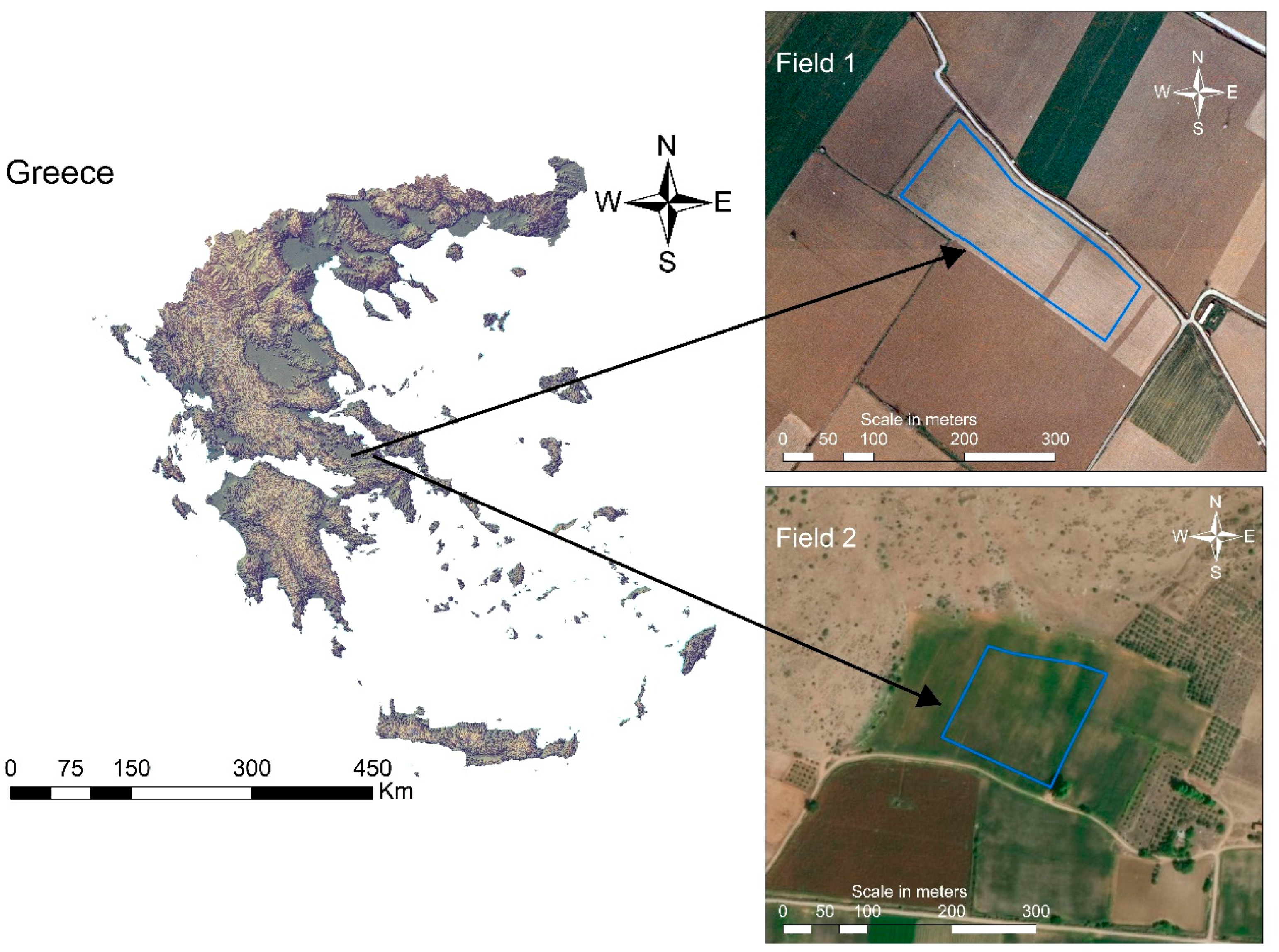
The study area was located in Chaeronea (38°29′44 N, 22°50′41 E), central Greece. Several visits to the area were conducted in order to visually inspect the cultivated land, meet local farmers, and further select the appropriate fields for the experimentation. Criteria for the selection of the fields were in-field soil, topographical variations, and favorable accessibility conditions for fieldwork. The final selection concerned two fields sown with cotton. In both pilot fields, the cotton variety sown was Celia, the distance between the rows was 95 cm, and the sowing density was 23 to 25 plants per meter. The area of the first field (Field 1) was 2.3 ha and it was completely flat, while the second one (Field 2) was a 1.9 ha sloped field (Figure 1). The experimental plan involved one growing period.
2.2. Data Acquisition
Data acquisition concerned a series of field operations that took place throughout an entire cultivation period of the two fields and concerned soil sampling, leaf sampling, and aerial image capturing.
2.2.1. Soil Samples
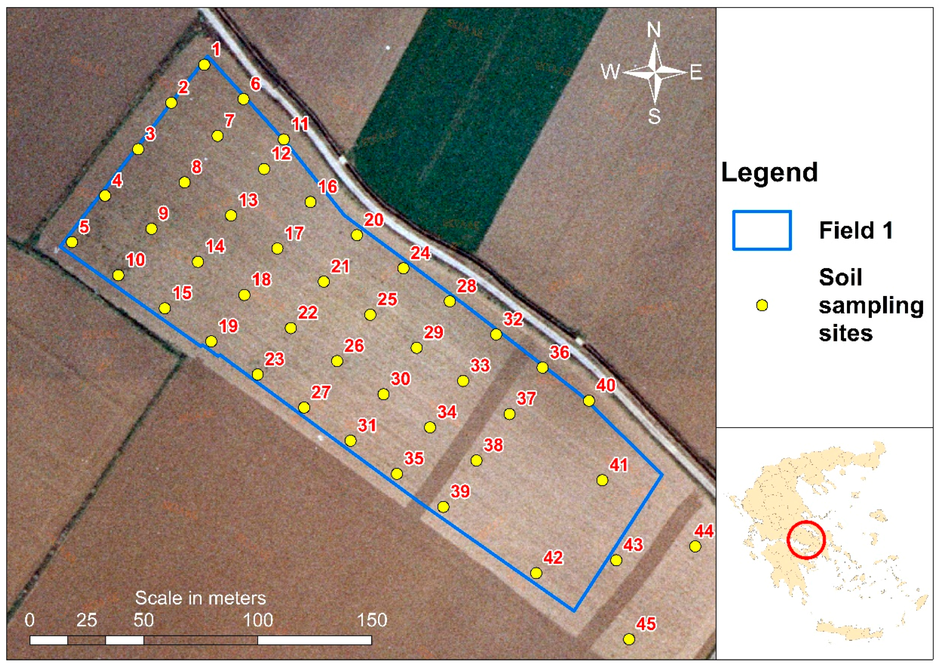
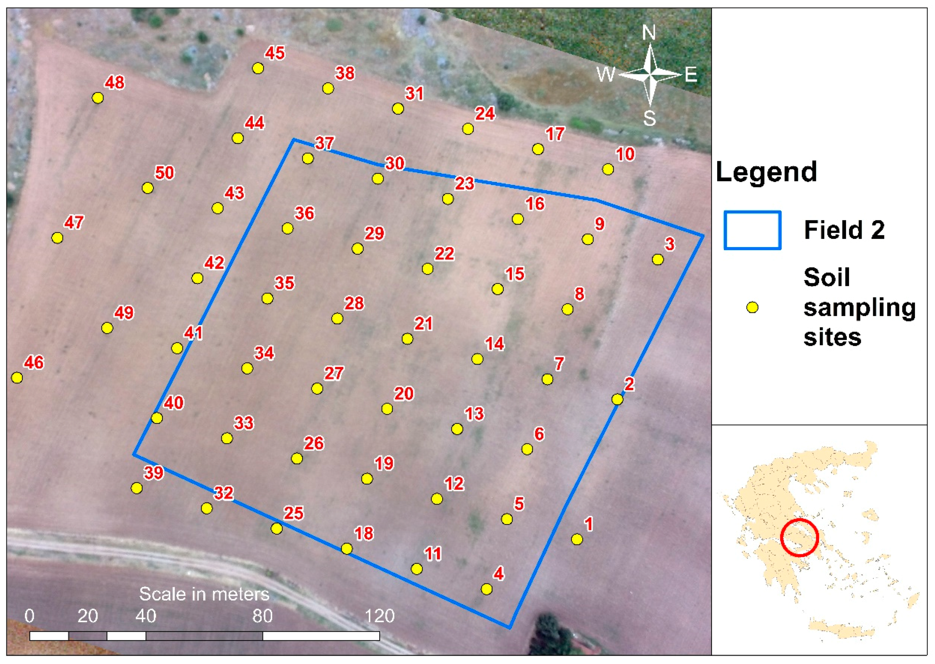
Preliminarily to soil sampling, a grid plan was compiled for each field based on two aerial photos of the fields, with the use of the GIS software package ArcGIS (ESRI Inc., California, USA). Grid pixel size was 25 m and, hence, the number of sampling positions was 45 in Field 1 and 50 in Field 2 (Figure 2 and Figure 3). In order to spatially cover as representatively as possible, the area of the two fields, several in-field sampling sites exceeded the grid boundaries. Soil sampling took place in April with the use of a standard soil auger. The depth of the soil samples was 0–30 cm. Soil physicochemical analyses included the measurement of soil texture (clay content), soil acidity (pH), calcium carbonate percentage (CaCO3), organic matter (OM), total nitrogen, and electrical conductivity (EC). The descriptive statistics of the aforementioned soil parameters per field are presented in Table 1 and Table 2.
2.2.2. Leaf Samples
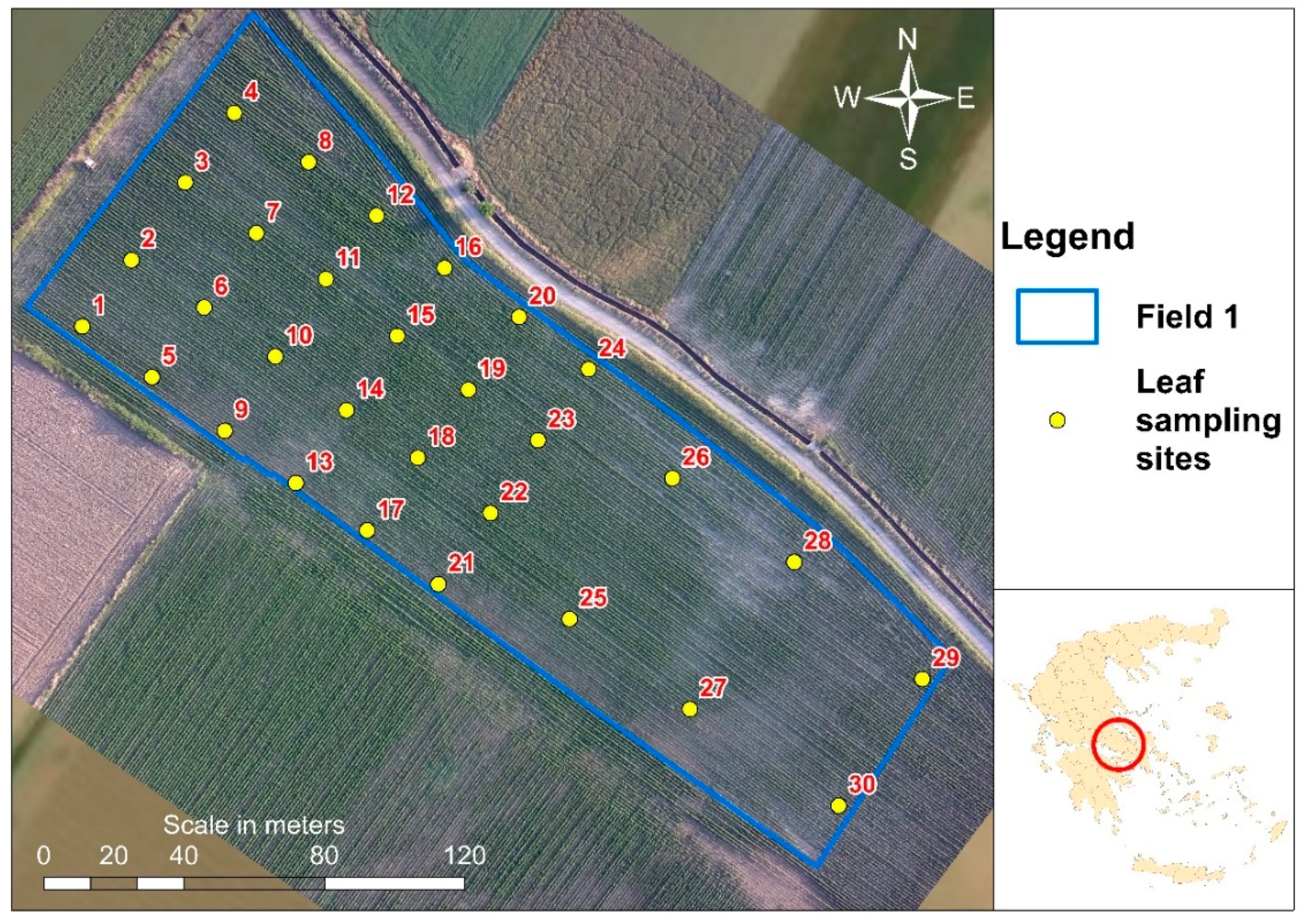
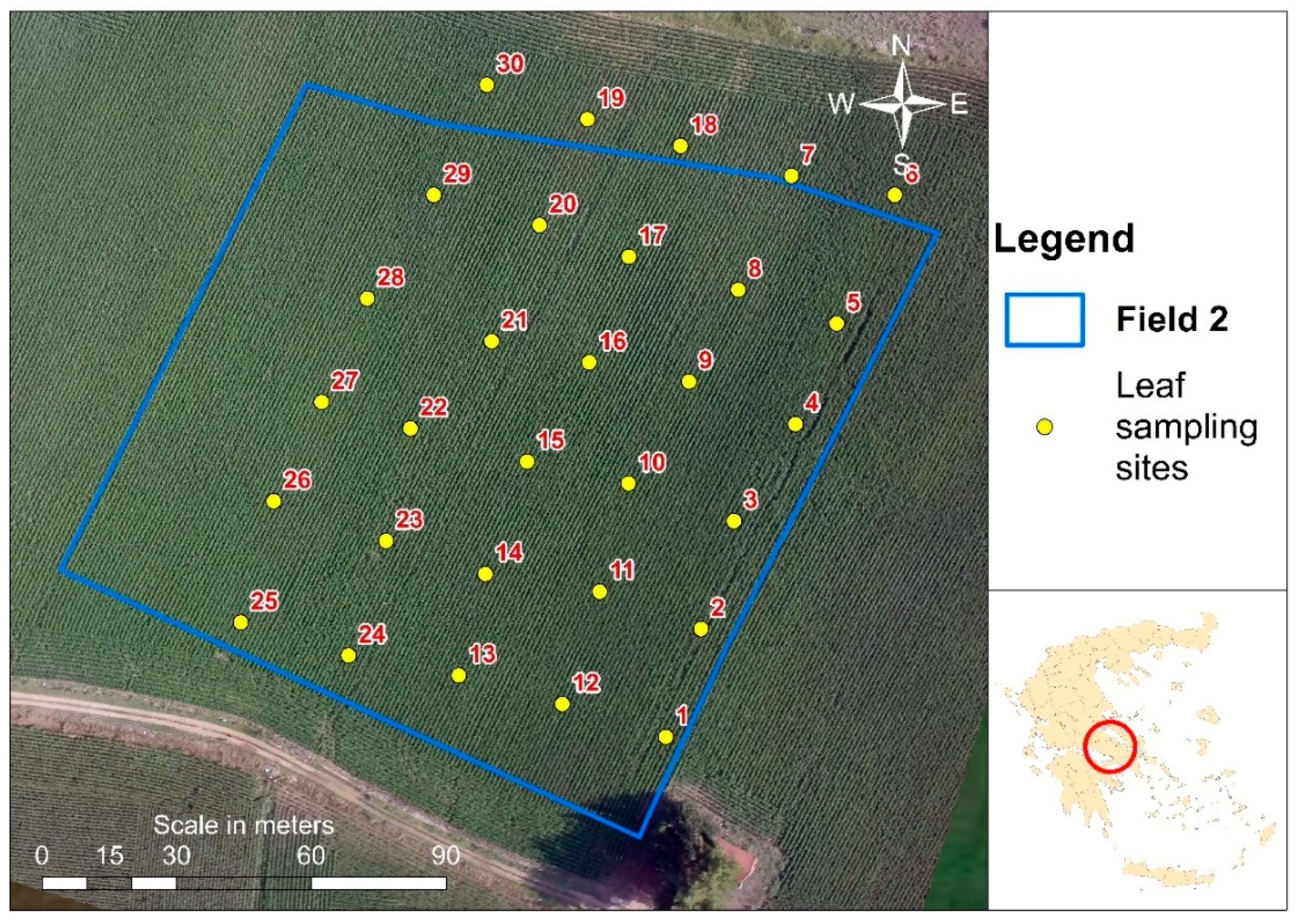
Leaf sampling in the study fields took place in July. Both cotton fields were at the full bloom stage, and each sample contained approximately 30 late mature leaves cut from different plants covering an area of one square meter around the sampling site. The number and the actual position of the sampling sites were based on the grid plan originally drawn for soil sampling, and regarded a subset of the respective soil samples. In each field, leaf samples were collected from 30 sites (Figure 4 and Figure 5). The leaves after cutting were put in paper bags and transferred to the laboratory for further analyses. The leaf samples were analyzed for total nitrogen, potassium, iron, copper, and zinc. The descriptive statistics of the macro and micronutrients measured in the cotton leaves in the two fields are presented in Table 3 and Table 4.
2.2.3. Aerial Data
Aerial data were captured with a UAS. The UAS comprised of a low-cost and low-weight quadcopter (Phantom, Da-Jiang Innovations (DJI) Science and Technology Co., Ltd., Shenzhen, China) and a 12-Megapixel (4000 × 3000 pixels) Hero digital camera (GoPro Inc., San Mateo, CA, USA), especially modified by Back-Bone Gear Inc., Ottawa Canada (Figure 6).
The camera’s stock lens was substituted by a flat lens (focal length 4.4 mm, relative aperture f/2.8, sensor size 1/2.3 inch and 71° angle of view). This modification was made in order to eliminate the distortion produced by fish-eye effect of the wide-angle lens [45]. Moreover, the modified camera was configured with removable filter positioning. Particularly, two detachable filters (IR-cut [400–700 nm] and near-infrared long-pass [715–1100 nm]) were used to capture aerial photographs in visible and near-infrared wavelengths, respectively.
The digital camera was attached to the quadcopter on a gimbal for compensating the quadcopter movement during flights and guaranteeing nadir image acquisition [46]. The camera was triggered before each flight mission to capture one image per 2 s. The quadcopter was equipped with the standard DJI flight control system, consisting of the main controller (MC), the inertial measurement unit (IMU), the global positioning system (GPS) receiver, and the compass. The quadcopter was remotely piloted through a 2.4 GHz radio control transmitter. Two flight missions per pilot field were scheduled and carried out. The first one was in April and the second in July, as close as possible to the dates of soil and plant sampling, respectively. The flights were carried out in stable cloud free ambient light conditions in the morning, at about 11:00 a.m. local time, at 250 m above ground level (AGL). The data collected by the UAS were two pairs of aerial images per pilot field and per flight date. Each pair consisted of one color composite (red–green–blue) image and one image in near-infrared wavelength. The selection of taking one image per field was made because photo stitching or orthomosaic generation would have introduced errors and artifacts in aerial data. The parameters used in all further analyses were the digital numbers (DN) of the aerial photos as captured in the near-infrared area of spectrum [47,48].
2.3. Data Management and Analysis
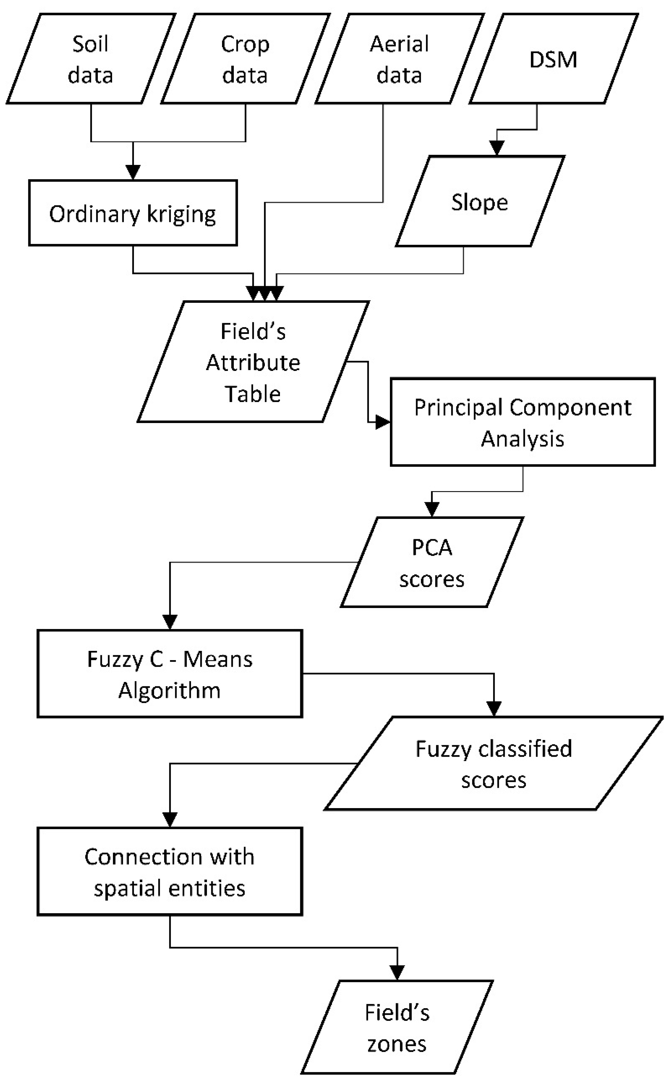
The soil parameters used in the analysis for Field 1 were those presented in Table 1, while for the analysis of Field 2, slope parameter (%) was included. Slope was calculated using an existing digital surface model (DSM) of the area. Respectively, the list of leaf parameters used is shown in Table 3. All data were georeferenced and stored in a geodatabase (ArcGIS, ESRI Inc., Redlands, CA, USA) for further processing. Data management concerned the harmonization of formats, meaning that all data were transformed into raster files. Point referenced data were converted into continuous raster surfaces with the use of ordinary kriging geostatistical method of interpolation [49]. Aerial imagery yet being in raster format needed no further transformation. Nevertheless, in order to correctly (and accurately) apply overlay spatial methods to all datasets, common pixel size (0.1 m) and grid size, starting point, and orientation were met. The raster files, after being overlaid, were extracted to a single attribute table per field, in which every row represented a pixel and every column contained the values of the parameters involved in each analysis.
The succeeded steps of the analysis were accomplished through a combination of principal component analysis (PCA) and of Fuzzy c-means algorithm application. PCA is a multivariate statistical technique that aims to reduce the dimensions of a multiparameter system, by recognizing linear combinations between its initial variables. It aims to not only reduce the number of initial data, but also to analyze and explore interrelations between them [50]. More specifically, PCA was executed using SPSS (IBM Corp., Armonk, NY, USA) in the attribute data of the two fields, in order to investigate possible relationships or groupings between those parameters. In the applied PCA, Varimax with Kaiser normalization method of rotation was selected, and Kaiser’s rule was decided for preserving the principal components [51,52]. PCA scores, accounting for every pixel of the combined raster file, underwent fuzzy classification using the Fuzzy c-means algorithm as applied in MATLAB software (MathWorks Inc., Natick, MA, USA). Fuzzy c-means classifies each participating value into a selected number of clusters with variable membership values ranging between 0 and 1. It is an unsupervised iterative algorithm that finds the cluster centroids of groups for which the in-cluster variability is minimized, whereas the between-cluster variability is maximized [53]. A flowchart of the methodological steps followed in the analysis is presented in Figure 7. The analysis shown in Figure 7 was followed twice for each field. Regarding Field 1, the first one was using soil and aerial data (April flight) and the second using crop and aerial data (July flight). Similarly, for Field 2 the analysis was run firstly with soil, slope, and aerial data (April flight), and secondly with crop, slope, and aerial data (July flight).
Fuzzy c-means was used in order to identify and further delineate in-field areas that possibly hold specific soil and crop characteristics and for which certain management strategies can be applied. Prior to the application of the algorithm, it was decided, in all cases (soil and crop characteristics), to preserve and output two zones per field for feasibility reasons in further managing them. Site-specific fertilizer management in order to be realistic and applicable should be adapted to farming conditions and to producers in terms of cost and labor effectiveness. However, except for practicality reasons, the final decision about the number of the management zones was also subject and yet controlled by the resulting between-zone variability or homogeneity in the analysis parameters.
2.4. Spatial Variability Analysis
Towards investigating and capturing the spatial variability in soil and plant parameters for both fields, semivariograms were calculated as part of the ordinary kriging interpolation method. The best-fitted models were identified, describing the spatial patterns of different properties. In Table 5, the results of semivariogram analysis are presented. According to Table 5, the best-fitted models in the studied properties differed from one field to another in five of eleven properties (EC, Organic Matter, Total Nitrogen in soil, Potassium and Copper). In the other six parameters (Clay, pH, CaCO3, Total Nitrogen in plant, Iron and Zinc) the models best fitted between the two fields were the same. The models selected, varied between spherical, pentaspherical, Gaussian, circular and exponential, reflecting the different spatial variability caused by the type of the property and also related to field conditions. A generic rule of thumb on which model is best linked to a specific soil or plant property, cannot be drawn from present analysis.
Based on the criterion that the ratio of nugget to sill is a measure of spatial dependency of the variables, according to Table 5, a large part of the variance in all parameters is introduced spatially. More specifically, as stated in [54], a ratio below 0.25 indicates strong spatial dependence in the variable. Following, the variance is medium if the ratio is between 0.25 and 0.75 and for ratio’s values above 0.75 the spatial dependence is weak. Clay content, EC, CaCO3, Total nitrogen in soil and in plants, Potassium, Iron in Field 1 and CaCO3, Total nitrogen in soil, Potassium and Iron in Field 2, showed a strong spatial dependence. Medium spatial variance was revealed among pH, Organic Matter, Zinc in Field 1 and Clay content, EC, pH, Organic Matter, Total nitrogen in plants and Zinc in Field 2. Finally, weak spatial dependence was attributed only to Copper concentration in both fields.
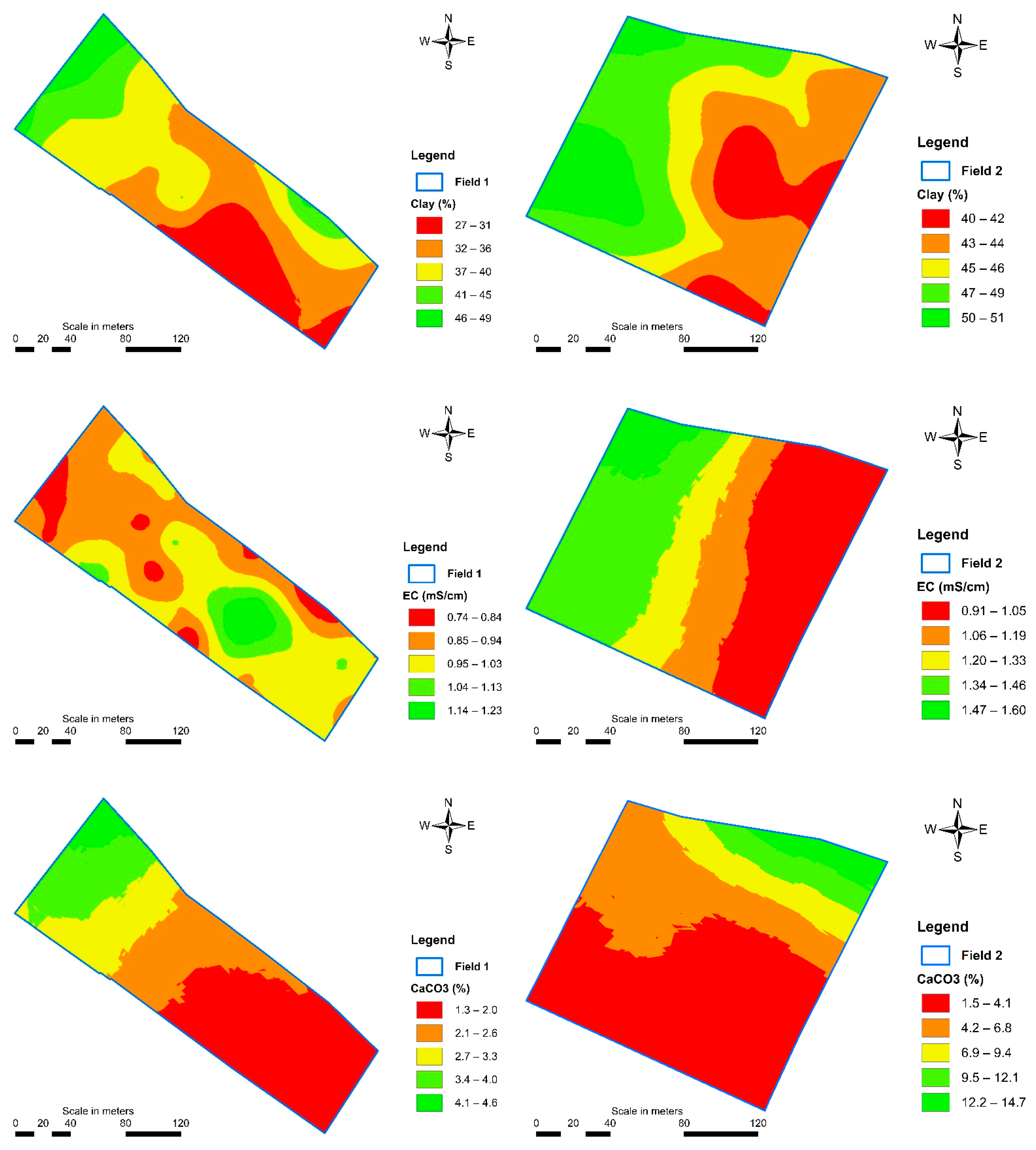
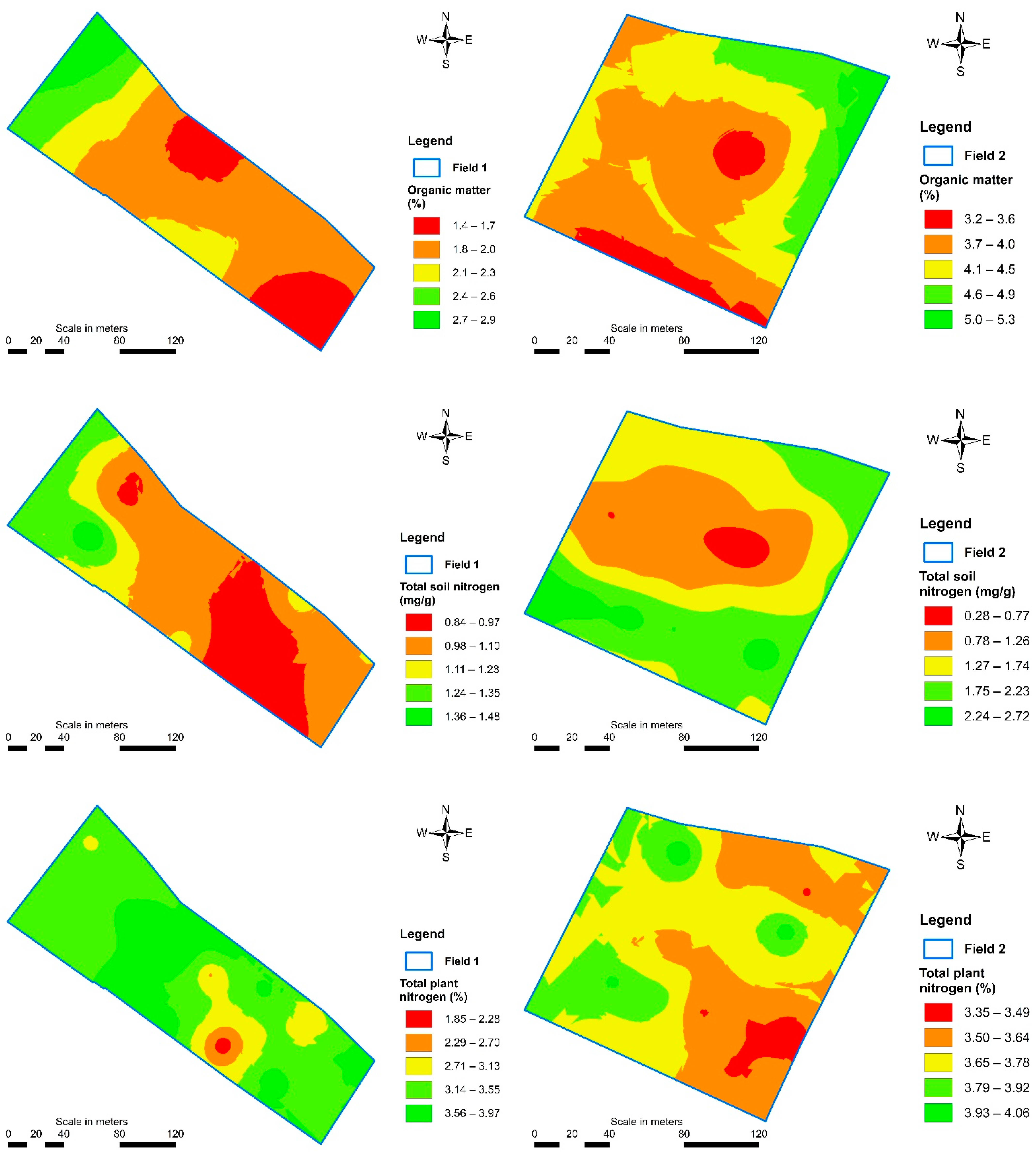
The spatially interpolated maps of Clay content, EC, CaCO3, Organic Matter, Total nitrogen in soil and in plants, Potassium and Iron in both fields exhibiting moderate to high spatial dependence are presented in Figure 8.
As far as soil properties are concerned, the northwestern part of Field 1 presents high values in clay percentage, carbonates, organic matter and total nitrogen, which can be attributed to its finer texture, while the southeastern area appears to retain lower values in these attributes. Electrical conductivity at the northwestern part of Field 1 presents some of the lowest estimated values, however low to medium values of EC are also widespread across the area of the field. On the other hand, in Field 2, electrical conductivity variability clearly follows the spatial structure of soil texture. Carbonates in Field 2, diminish from northeast to south, while organic matter and total nitrogen set a low value area, approximately at the middle of the field. Regarding plant properties, in both fields, total nitrogen and potassium concentration present only few scattered low spot areas, while the range between minima and maxima is not quite notable. Iron concentration in leaf samples on both fields however, reveals distinct spatial patterns. In Field 1, low concentration areas appear at northwestern, center and southeastern parts of the field and only two areas of high values appear mainly at the northern and western segments of the field. In case of Field 2, it is almost divided into two areas, based on iron concentration, one at northeast holding low values, and another at south to southeast having higher iron values.
Geospatial analysis of each studied parameter revealed valuable information on the way each variable fluctuates across space, and can serve in guiding soil and leaf sampling schemes. Moreover, the combined effect of all parameters along with near-infrared spectral data and slope variable were investigated and realized through PCA and fuzzy clustering methodology as presented in Figure 7.
3. Results and Discussion
3.1. Soil Characteristics
The degree of correlation between soil parameters, slope, and NIR as participated in the analysis was defined through Pearson coefficient (r) calculation. The correlation matrix is presented in Table 6. The majority of the parameters were correlated with each other in both fields. In Field 1, NIR was significantly and negatively correlated with clay content, organic matter, carbonates, and total soil nitrogen, while it was positively correlated with electrical conductivity. In Field 2, NIR shown significant negative correlation only with total soil nitrogen. On the other hand, increases in organic matter, carbonates, and soil acidity in Field 2 seem to increase NIR digital values. This diverse effect between the two fields may be attributed to noise in NIR values coming from existing weed patches and stones in the surface of Field 2. Among soil variables, electrical conductivity was negatively correlated with pH, organic matter, carbonates, total soil nitrogen in both fields, and with clay content in Field 1, which was also noted in spatial variability analysis (Figure 8). In Field 2, clay content was positively correlated with electrical conductivity and organic matter with carbonates and total soil nitrogen. Slope parameter was also correlated with all soil variables except for organic matter.
Correlations among soil parameters, slope, and NIR indicated that PCA could be performed to aggregate those variables that set the main sources of variability across the fields.
In the case of Field 1, the principal components selected, were the first two according to the Kaiser criterion. Their eigenvalue was higher than 1 and the cumulative variance explained by those two components was higher than 72% of the total variance in the initial parameters (Table 7). More specifically, the first component accounts for 57.6% of total variance while the second one adds further 15.3% in the variance explained by the components extracted.
Table 8 presents each principal component’s loadings. According to Table 8, the first component aggregates near-infrared (NIR) parameter with all soil parameters except for soil acidity (pH), which is highly correlated with the second component axis. This means, that NIR value monitoring and recording may infer crucial results regarding spatial variability in soil characteristics. It is also noticed that the values of NIR along with the conductivity of soil samples are grouped in the negative part of first component’s axis, having the opposite influence on the component than that of the other soil parameters. This practically means that under the conditions of the first pilot field the variance of NIR values across the field is followed by the variance in electrical conductivity and inversely relates to the variability of the other five soil parameters, namely clay content, pH, CaCO3, OM, and total nitrogen.
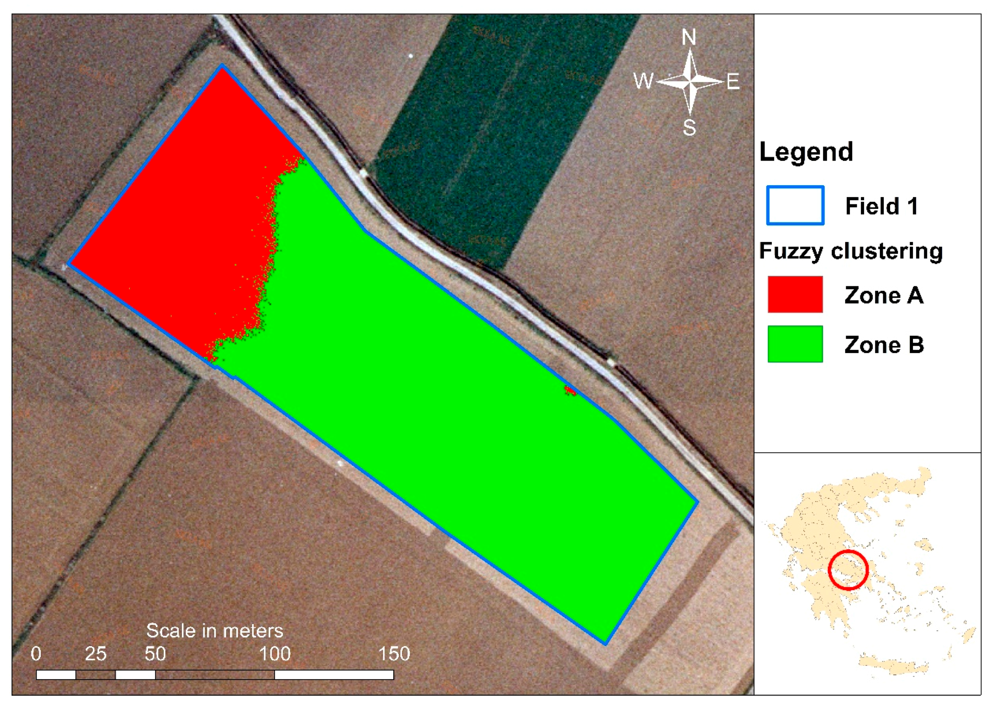
Table 8 findings, in essence, constitute two linear combinations of the initial parameters with the resulting principal components, where the loadings represent the equations’ coefficients. Subsequently, “solving” each equation for every single pixel, holding all seven values participating in the analysis, a pair of “scores” per pixel is calculated. Those pairs were introduced in Fuzzy c-means algorithm thus ascribing each pixel to a certain category according to its attributed, by the algorithm, membership value. The resulting layout, as produced in ArcGIS, is presented in Figure 9. In Figure 9 and according to the analysis applied in soil and reflectance parameters, Field 1 is divided into two zones (A and B). Zone A preserves higher percentages in organic matter, clay content and carbonates comparing to Zone B. Electrical conductivity is lower in Zone A than in B while total nitrogen content is slightly higher and soil acidity’s difference is negligible. Mean values of all soil properties except for total nitrogen and pH were statistically different (p < 0.01) between the two zones (Table 9). Comparing Ζones Α and Β, based on Table 9 results, Ζone Α presents better growth conditions for cotton plants as it can promote nutrient and moisture availability.
Regarding Field 2, PCA extracted in a total of eight components, of which the first three were selected representing 87.3% of the variance in the initial parameters, meaning that, counting only three variables, i.e., the three components, the variability of the eight initial factors can be fairly explained. The first component represents 41.4% of the variance in the participating variables, the second one adds 29.3%, and the third one contributes another 16.5% (Table 10).
Consequently, the loadings of the two principal components for Field 2 are presented in Table 11. In the case of Field 2, the parameter of NIR is classified into the second component, forming a group with organic matter and carbonates. As previously mentioned, these two soil chemical parameters appear to be aggregated in the analysis of Field 1, along with the clay variable, which, in Field 2, is clearly grouped with electrical conductivity under the first component. The latter in soil substrate can be explained by the fact that heavy soils, rich in clay content, appear to have bad drainage conditions, which can cause the accumulation of salts and, thus, raise soil electrical conductivity. In contrary to Field 1, under Field 2 conditions, NIR parameter seems to drive positively the second component similarly to organic matter and carbonate content. The introduction of slope variable in the analysis may have caused this differentiation, which does not retain clear participation in any of the three components. Total nitrogen has excluded itself from the first two components, designating the third one, denoting that, under the conditions of this analysis, does not associate with the other soil variables.
The respective mapping layout of the fuzzy clustering procedure is presented in Figure 10.
In Table 12, the mean values of the seven participating parameters per extracted zone in Field 2 are presented. Statistically (p < 0.01), the mean values of clay content, electrical conductivity, organic matter, carbonates, and slope were significantly different. Zone B, according to Table 12, had significantly higher mean value in carbonates and slightly higher in organic matter than Zone A. The other parameters’ mean values did not appear to differ among the two parts of the field; however, the slope in Zone B was greater than in Zone A. Soil conditions in Field 2, either in Zone A or in B, set no limitation for cotton growth. However, the resulting delineation of the zones can serve as a guide for future soil and fertilizing management practices. Further, as outputted by the statistical means between zones in both fields, the two-zone approach, may offer an acceptable trade-off between practicality and variability highlighting.
3.2. Crop Characteristics
Table 13 presents the degree of correlation among plant parameters, slope, and NIR digital values in Fields 1 and 2. NIR demonstrated weak correlation with all parameters; however, plant variables among each other exhibited significant correlations. Notable is the negative relation of total plant nitrogen with potassium and copper and the positive one with iron and slope in Field 2. Further, copper was positively correlated with potassium in Field 1 and with zinc in Field 2. Potassium in cotton leaves was also negatively correlated with slope percentage in Field 2. Despite the statistically insignificant correlation of NIR with crop variables, PCA should be applied in order to reveal groupings and variances among data.
The application of PCA in regards to parameters derived from plant tissue analysis in conjunction with NIR values taken by air, resulted in data presented in Table 14. Six components were calculated, among which, the first three cumulatively explain almost 69% of the variability in the initial data. This is a rather weak percentage judging by the fact that the parameters involved were only six and the selected components were three, thus reducing the dimensions of the analysis only by 50%. However, the first two components can explain 51.5% of the variance in the parameters engaged.
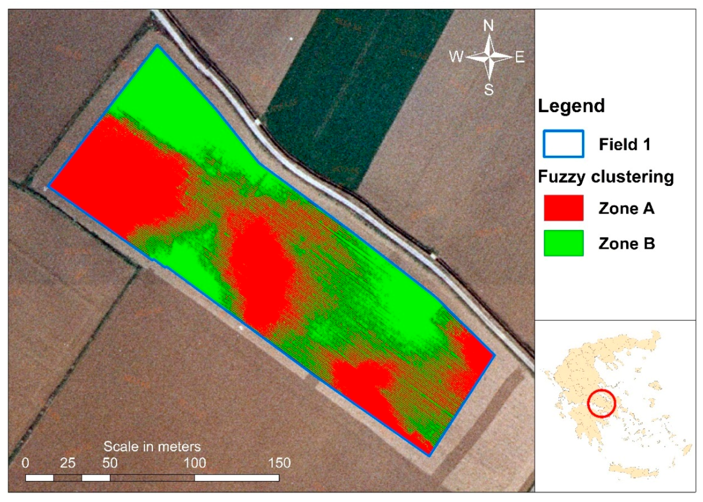
Furthermore, a few groupings were revealed, as shown in Table 15. In fact, potassium and copper concentrations in cotton plants were associated with the first principal component, total nitrogen and zinc concentration had high correlation with the second one, and NIR values, followed by iron concentration were grouped under the third component. It is clear that, under the specific dataset, the NIR parameter cannot be used for drawing safe conclusions about the spatial distribution of the nutrient composition of the plants throughout Field 1. The mapping of the fuzzy classification led to the layout presented in Figure 11. Contrary to the zones extracted by the soil characteristic analysis (Figure 9), here the zones are not aggregated in specific parts of the field, but the sub-areas are scattered across the field. It is also noticeable that the algorithm even classified cotton rows into the two zones. For this reason, the proposition of site-specific management strategies regarding crop nutrition is rather difficult to be applied.
Further, it is argued that, according to the results presented in Table 16, clustering did not manage to discriminate areas of clear variability between the crop parameters measured, except for iron concentration, in which statistically significant differences (p < 0.01) in mean values per zone were recorded. Zone B appears to retain higher mean values of iron comparing to Zone A, however, being at absolute values that set no risk of future deficiencies in the plants.
In the case of Field 2, with the inclusion of slope percentage, the analysis extracted seven components from which the first three accounted for 72.6% of the variance in the data (Table 17). The NIR parameter seems to have low contribution to all of the three components; however, according to its loadings, tends to group under the first component. This states its slight correlation with the other parameters measured. The variables of slope and potassium concentration are also grouped under the first component having high absolute loadings. The loadings of zinc and copper clearly differentiate from the other parameters, characterizing the second component, while the third component is dominated by an iron parameter and, at a lesser degree, by total nitrogen (Table 18).
According to the results of PCA in crop characteristics, NIR did not group in sufficient rate with the other parameters in Field 1 and in Field 2. A possible explanation is the fact that all nutrients measured in cotton plants in both fields were at sufficient levels and their value variations along the area of the fields were not significant. Due to this uniformity, the variability of aerial NIR values was also low, which was reflected in the output of PCA.
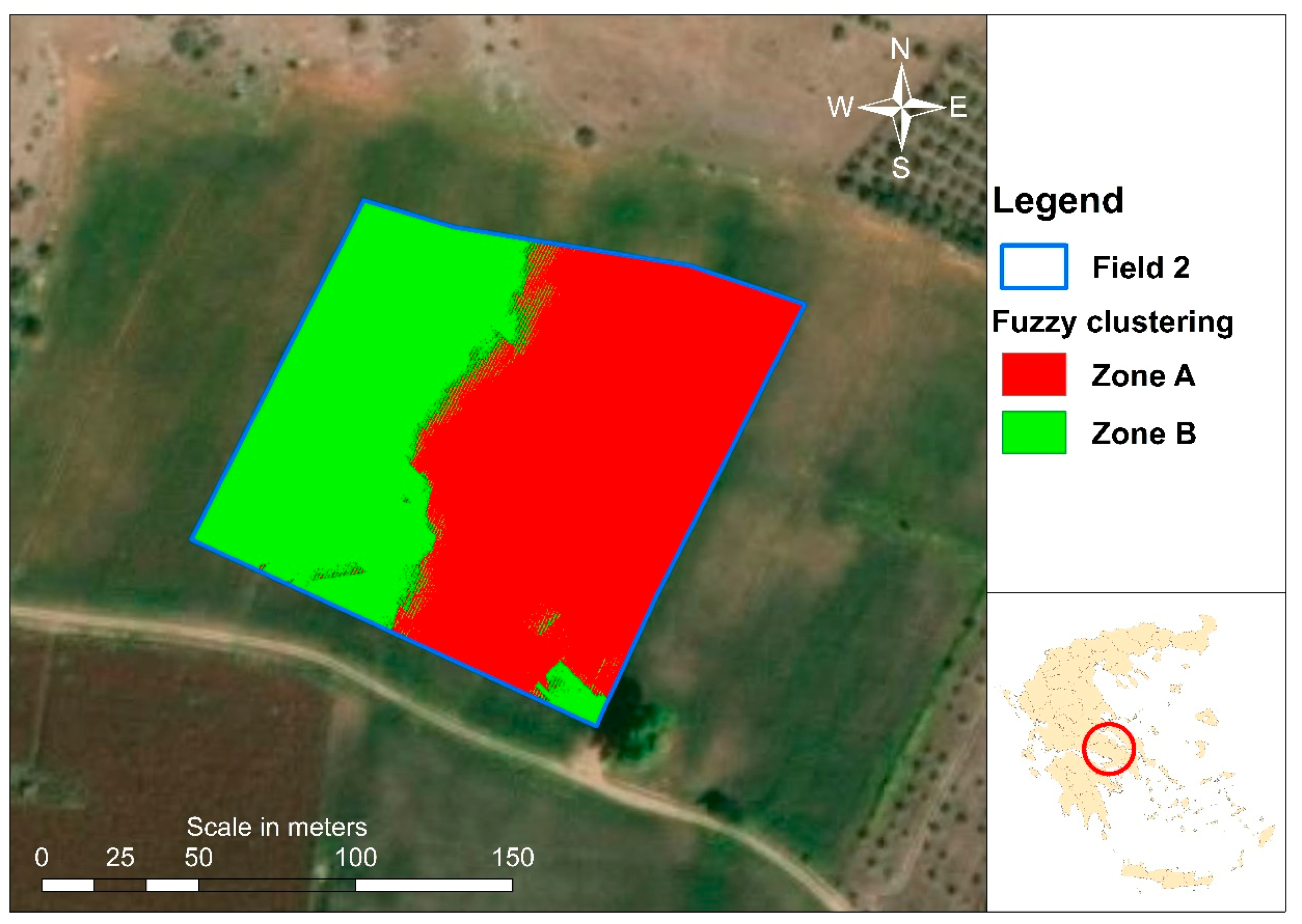
The mapping layout of the Fuzzy c-means output regarding Field 2 is shown in Figure 12. Visually, there is a clear delineation of two zones, one at the left-hand side and the other at the right of the field. The bottom right corner of the field being classified in Zone B is possibly attributed to the shade effect that a nearby tree had on the background reflectance, and it is considered an image artifact.
4. Conclusions
In the context of this study, UAS data were analyzed with soil and crop parameters in two cotton fields during a growing period. All data were analyzed using geostatistical and geospatial methodologies coupled with PCA and Fuzzy c-means clustering under GIS environment. A primary conclusion, of practical importance is that the use of UAS in crop production offers a quick and reliable way to monitor soil and plant capital. As many UAS manufacturers throw their products into the market, raising competition, and diminishing costs, many farmers are able to engage UAS or similar services to their production procedure. Another finding is that fieldwork, in the form of sampling and further analyzing soil and tissue samples, are of crucial importance for evaluating and confirming remotely sensed data. This work demonstrated that reflectance data were correlated with organic matter, carbonate, and clay content, while those data can be directly used for in-field zone delineation. This time efficient form of field monitoring can lead to targeted sampling schemes, avoiding unnecessary work and costs. On the contrary, crop nutrient characteristics were insignificantly combined with aerial data, which may have been the result of uniformity of the measured parameters across the two fields. The resulting zones, as mapped in this case, offer little in fertilizing management guidance. Further work should evaluate present results by incorporating more fields, crops, and growing seasons. Research efforts should also focus on translating the outcomes of soil and crop monitoring through expert decision-making tools and on efficiently applying management plans through variable rate technologies. The integration of new technologies and established methodologies in primary production, such as those demonstrated, provide notable means for applying site-specific crop management in broader adoption levels and constitute a crucial motive for visualizing, designing, implementing, and assessing environmental strategic plans towards a circular economy.
Author Contributions
Conceptualization, A.V.P.; methodology, A.V.P. and D.P.K.; validation A.V.P.; investigation, A.V.P.; writing—original draft preparation A.V.P.; writing—review and editing, D.P.K. and A.V.P.; visualization, A.V.P.; supervision, A.V.P. and D.P.K. All authors have read and agreed to the published version of the manuscript.
Funding
The research project was co-funded by the European Social Fund and by National Resources through the National Strategic Reference Framework 2007–2013 (NSRF 2007–2013).
Data Availability Statement
The data are not publicly available due to privacy.
Conflicts of Interest
The authors declare no conflict of interest.
References
- Shao, Y.; Peng, G.; Leslie, L.M. The Environmental Dynamic System. In Environmental Modelling and Prediction; Peng, G., Leslie, L.M., Shao, Y., Eds.; Springer: Berlin/Heidelberg, Germany, 2002. [Google Scholar] [CrossRef]
- Lichtenberg, E. Agriculture and the environment. In Handbook of Agricultural Economics; Elsevier: Amsterdam, The Netherlands, 2002; Volume 2. [Google Scholar]
- Escolano, J.J.; Navarro-Pedreño, J.; Gómez Lucas, I.; Almendro-Candel, M.B.; Zorpas, A.A. Decreased organic carbon associated with land management in Mediterranean environments. In Soil Management and Climate Change: Effects on Organic Carbon, Nitrogen Dynamics and Greenhouse Gas Emissions; Muñoz, M.A., Zornoza, R., Eds.; Academic Press: Cambridge, MA, USA, 2018. [Google Scholar] [CrossRef]
- Navarro-Pedreño, J.; Almendro-Candel, M.B.; Zorpas, A.A. The Increase of Soil Organic Matter Reduces Global Warming, Myth or Reality? Preprints 2020, 2020120100. [Google Scholar] [CrossRef]
- Bongiovanni, R.; Lowenberg-Deboer, J. Precision Agriculture and Sustainability. Precis. Agric. 2004, 5, 359–387. [Google Scholar] [CrossRef]
- Plant, R.E. Site-specific management: The application of information technology to crop production. Comput. Electr. in Agric. 2001, 30, 9–29. [Google Scholar] [CrossRef]
- Khanna, M.; Epouhe, O.F.; Hornbaker, R. Site-Specific Crop Management: Adoption Patterns and Incentives. Appl. Econ. Perspect. Policy 1999, 21, 455–472. [Google Scholar] [CrossRef]
- Campbell, J.B. Spatial Variability of Soils. Ann. Assoc. Am. Geogr. 1979, 69, 54–4556. [Google Scholar] [CrossRef]
- Hanquet, B.; Sirjacobs, D.; Destain, M.F. Analysis of Soil Variability Measured with a Soil Strength Sensor. Precis. Agric. 2004, 5, 227–246. [Google Scholar] [CrossRef]
- Stadler, A.; Rudolph, S.; Kupisch, M.; Langensiepen, M.; van der Kruk, J.; Ewert, F. Quantifying the effects of soil variability on crop growth using apparent soil electrical conductivity measurements. Eur. J. Agron. 2015, 64, 8–20. [Google Scholar] [CrossRef]
- Ji, W.; Adamchuk, V.I.; Chen, S.; Mat Su, A.S.; Ismail, A.; Gan, Q.; Shi, Z.; Biswas, A. Simultaneous measurement of multiple soil properties through proximal sensor data fusion: A case study. Geoderma 2019, 341, 111–128. [Google Scholar] [CrossRef]
- Viscarra Rossel, R.A.; Lobsey, C.R.; Sharman, C.; Flick, P.; McLachlan, G. Novel Proximal Sensing for Monitoring Soil Organic C Stocks and Condition. Environ. Sci. Technol. 2017, 51, 5630–5641. [Google Scholar] [CrossRef] [Green Version]
- Meléndez Pastor, I.; Navarro-Pedreño, J.; Gómez Lucas, I.; Zorpas, A.A. A model for evaluating soil vulnerability to erosion using remote sensing data and a fuzzy logic system. In Modern Fuzzy Control Systems and Its Applications; Ramakrirshnan, S., Ed.; Intech Open Science: Rijeka, Croatia, 2017; Chapter 21; pp. 437–545. [Google Scholar] [CrossRef] [Green Version]
- Arnó, J.; Rosell, J.R.; Blanco, R. Spatial variability in grape yield and quality influenced by soil and crop nutrition characteristics. Precis. Agric. 2012, 13, 393–410. [Google Scholar] [CrossRef] [Green Version]
- Navarro-Pedreño, J.; Almendro Candel, M.B.; Gómez Lucas, I.; Jordán Vidal, M.M.; Borrás, J.B.; Zorpas, A.A. Trace metal content and availability of essential metals in agricultural soils of a Mediterranean region related to soil properties. Sustainability 2018, 10, 4534. [Google Scholar] [CrossRef] [Green Version]
- Taylor, J.C.; Wood, G.A.; Earl, R.; Godwin, R.J. Soil Factors and their Influence on Within-field Crop Variability, Part II: Spatial Analysis and Determination of Management Zones. Biosyst. Eng. 2003, 84, 441–453. [Google Scholar] [CrossRef]
- Ziliani, M.G.; Parkes, S.D.; Hoteit, I.; McCabe, M.F. Intra-Season Crop Height Variability at Commercial Farm Scales Using a Fixed-Wing UAV. Remote Sens. 2007, 10. [Google Scholar] [CrossRef] [Green Version]
- Korhonen, J.; Honkasalo, A.; Seppälä, J. Circular Economy: The Concept and its Limitations. Ecol. Econ. 2018, 143, 37–46. [Google Scholar] [CrossRef]
- Tseng, M.-L.; Chiu, A.S.F.; Chien, C.-F.; Tan, R.R. Pathways and barriers to circularity in food systems, Resources. Conserv. Recycl. 2019, 143, 236–237. [Google Scholar] [CrossRef]
- Antoniou, N.; Zorpas, A.A. Quality Protocol Development to define End-of-Waste Criteria for Tire Pyrolysis Oil in the framework of Circular Economy Strategy. Waste Manag. 2019, 95, 161–170. [Google Scholar] [CrossRef]
- Barros, M.V.; Salvador, R.; de Francisco, A.C.; Piekarski, C.M. Mapping of research lines on circular economy practices in agriculture: From waste to energy. Renew. Sustain. Energy Rev. 2020, 131, 109958. [Google Scholar] [CrossRef]
- Vardopoulos, I.; Konstantopoulos, I.; Zorpas, A.A.; Limousy, L.; Bennici, S.; Inglezakis, V.; Voukkali, I. Sustainable metropolitan areas perspectives though the assessment of the existing waste management strategy. Environ. Sci. Pollut. Res. 2020. [Google Scholar] [CrossRef]
- Loizia, P.; Neofytou, N.; Zorpas, A.A. The concept of circular economy in food waste management for the optimization of energy production through UASB reactor. Environ. Sci. Pollut. Res. 2019. [CrossRef]
- Zorpas, A.A. Strategy Development in the Framework of Waste Management. Sci. Total Environ. 2020, 716, 137088. [Google Scholar] [CrossRef]
- Loizia, P.; Voukali, I.; Zorpas, A.A.; Navarro-Pedreño, J.; Chatziparaskeva, G.; Inglezakis, V.J.; Vardopoulos, I.; Doula, M.K. Measuring the level of environmental performance in insular areas, through key performed indicators, in the framework of waste strategy development. Sci. Total Environ. 2021, 753, 141974. [Google Scholar] [CrossRef] [PubMed]
- Doula, M.K.; Zorpas, A.A.; Inglezakis, V.J.; Navarro-Pedreño, J. Optimization of Soil behaviour after from 12 years disposed of Olive Mile Waste through the Implementation of Natural Clinoptilolite. J. Environ. Eng. Manag. 2019, 18, 1297–1309. [Google Scholar] [CrossRef]
- Pérez-Gimeno, A.; Navarro-Pedreño, J.; Almendro-Candel, B.M.; Gómez, I.; Zorpas, A.A. Characteristics of organic and inorganic wastes for their use in land restoration. Waste Manag. Res. 2019, 37, 502–507. [Google Scholar] [CrossRef] [PubMed] [Green Version]
- Voukali, I.; Loizia, P.; Navarro-Pedreño, J.; Zorpas, A.A. Urban Strategies Evaluation for Waste Management in Coastal Areas in the framework of area metabolism. Waste Manag. Res. 2021, in press. [Google Scholar] [CrossRef] [PubMed]
- Whelan, B. Site-Specific Crop Management. In Pedometrics. Progress in Soil Science; McBratney, A., Minasny, B., Stockmann, U., Eds.; Springer: Cham, Switzerland, 2018. [Google Scholar] [CrossRef]
- Shafian, S.; Rajan, N.; Schnell, R.; Bagavathiannan, M.; Valasek, J.; Shi, Y. Unmanned aerial systems-based remote sensing for monitoring sorghum growth and development. PLoS ONE 2018, 13. [Google Scholar] [CrossRef] [Green Version]
- Dong, T.; Shang, J.; Liu, J. Using RapidEye imagery to identify within-field variability of crop growth and yield in Ontario, Canada. Precis. Agric. 2019, 20, 1231–1250. [Google Scholar] [CrossRef]
- Khaliq, A.; Comba, L.; Biglia, A.; Ricauda Aimonino, D.; Chiaberge, M.; Gay, P. Comparison of Satellite and UAV-Based Multispectral Imagery for Vineyard Variability Assessment. Remote Sens. 2019, 11, 436. [Google Scholar] [CrossRef] [Green Version]
- Weiss, M.; Jacob, F.; Duveiller, G. Remote sensing for agricultural applications: A meta-review. Remote Sens. Environ. 2020, 236. [Google Scholar] [CrossRef]
- Maes, W.H. and Steppe, K. Perspectives for Remote Sensing with Unmanned Aerial Vehicles in Precision Agriculture. Trends Plant Sci. 2019, 24, 152–164. [Google Scholar] [CrossRef]
- Barbedo, J.G.A. A Review on the Use of Unmanned Aerial Vehicles and Imaging Sensors for Monitoring and Assessing Plant Stresses. Drones 2019, 3, 40. [Google Scholar] [CrossRef] [Green Version]
- Green, D.R. Remote sensing, GIS, the geospatial technologies, and Unmanned Airborne Vehicles at Aberdeen University. Scott. Geogr. J. 2019. [Google Scholar] [CrossRef]
- Shit, P.K.; Bhunia, G.S.; Maiti, R. Spatial analysis of soil properties using GIS based geostatistics models. Model. Earth Syst. Environ. 2016, 2, 107. [Google Scholar] [CrossRef] [Green Version]
- Denton, O.A.; Aduramigba-Modupe, V.O.; Ojo, A.O.; Adeoyolanu, O.D.; Are, K.S.; Adelana, A.O.; Oyedele, A.O.; Adetayo, A.O.; Oke, A.O. Assessment of spatial variability and mapping of soil properties for sustainable agricultural production using geographic information system techniques (GIS). Cogent Food Agric. 2017, 3. [Google Scholar] [CrossRef]
- Usowicz, B.; Lipiec, J. Spatial variability of soil properties and cereal yield in a cultivated field on sandy soil. Soil Tillage Res. 2017, 174, 241–250. [Google Scholar] [CrossRef]
- Valverde Arias, O.; Garrido, A.; Villeta, M.; Tarquis, A.M. Homogenisation of a soil properties map by principal component analysis to define index agricultural insurance policies. Geoderma 2018, 311, 149–158. [Google Scholar] [CrossRef]
- Metwally, M.S.; Shaddad, S.M.; Liu, M.; Yao, R.-J.; Abdo, A.I.; Li, P.; Jiao, J.; Chen, X. Soil Properties Spatial Variability and Delineation of Site-Specific Management Zones Based on Soil Fertility Using Fuzzy Clustering in a Hilly Field in Jianyang, Sichuan, China. Sustainability 2019, 11, 7084. [Google Scholar] [CrossRef] [Green Version]
- Aggelopoulou, K.; Castrignanò, A.; Gemtos, T.; de Benedetto, D. Delineation of management zones in an apple orchard in Greece using a multivariate approach. Comput. Electr. Agric. 2013, 90, 119–130. [Google Scholar] [CrossRef]
- Tripathi, R.; Nayak, A.K.; Shahid, M.; Lal, B.; Gautam, P.; Raja, R.; Mohanty, S.; Kumar, A.; Panda, B.B.; Sahoo, R.N. Delineation of soil management zones for a rice cultivated area in eastern India using fuzzy clustering. Catena 2015, 133, 128–136. [Google Scholar] [CrossRef]
- Peralta, N.R.; Costa, J.L.; Balzarini, M.; Franco, M.C.; Cordoba, M.; Bullock, D. Delineation of management zones to improve nitrogen management of wheat. Comput. Electr. Agric. 2015, 110, 103–113. [Google Scholar] [CrossRef]
- Shah, S.; Aggarwal, J.K. Intrinsic parameter calibration procedure for a (high-distortion) fish-eye lens camera with distortion model and accuracy estimation. Pattern Recognit. 1996, 29, 1775–1788. [Google Scholar] [CrossRef]
- Bendig, J.; Bolten, A.; Bareth, G. UAV-based imaging for multi-temporal, very high resolution crop surface models to monitor crop growth variability. PFG 2013, 6, 0551–0562. [Google Scholar] [CrossRef]
- Aldana-Jague, E.; Heckrath, G.; Macdonald, A.; van Wesemael, B.; van Oost, K. UAS-based soil carbon mapping using VIS-NIR (480–1000 nm) multi-spectral imaging: Potential and limitations. Geoderma 2016, 275, 55–66. [Google Scholar] [CrossRef]
- Papadopoulos, A.; Kalivas, D.; Theocharopoulos, S. Spatio-temporal monitoring of cotton cultivation using ground-based and airborne multispectral sensors in GIS environment. Environ. Monit. Assess. 2017, 189, 323. [Google Scholar] [CrossRef] [PubMed]
- Oliver, M.A.; Webster, R. Kriging: A method of interpolation for geographical information systems. Int. J. Geogr. Inf. Syst. 1990, 4, 313–332. [Google Scholar] [CrossRef]
- Jolliffe, I.T. Principal Component Analysis; Springer: Berlin, Germany, 1986. [Google Scholar] [CrossRef]
- Kaiser, H.F. The Application of Electronic Computers to Factor Analysis. Educ. Psychol. Meas. 1960, 20, 141–151. [Google Scholar] [CrossRef]
- Manly, B.F.J.; Navarro Alberto, J.A. Multivariate Statistical Methods: A Primer, 4th ed.; CRC Press: Boca Raton, FL, USA, 2016. [Google Scholar]
- Bezdek, J.C.; Ehrlich, R.; Full, W. FCM: The fuzzy c-means clustering algorithm. Comput. Geosci. 1984, 10, 191–203. [Google Scholar] [CrossRef]
- Cambardella, C.A.; Moorman, T.B.; Novak, J.M.; Parkin, T.B.; Turco, R.F.; Konopka, A.E. Field-scale variability of soil properties in central Iowa soils. Soil Sci. Soc. Am. J. 1994, 58, 1501–1511. [Google Scholar] [CrossRef]
Figure 1.
Study area and the two pilot fields.

Figure 2.
Soil sampling sites in Field 1.

Figure 3.
Soil sampling sites in Field 2.

Figure 4.
Leaf sampling sites in Field 1.

Figure 5.
Leaf sampling sites in Field 2.

Figure 6.
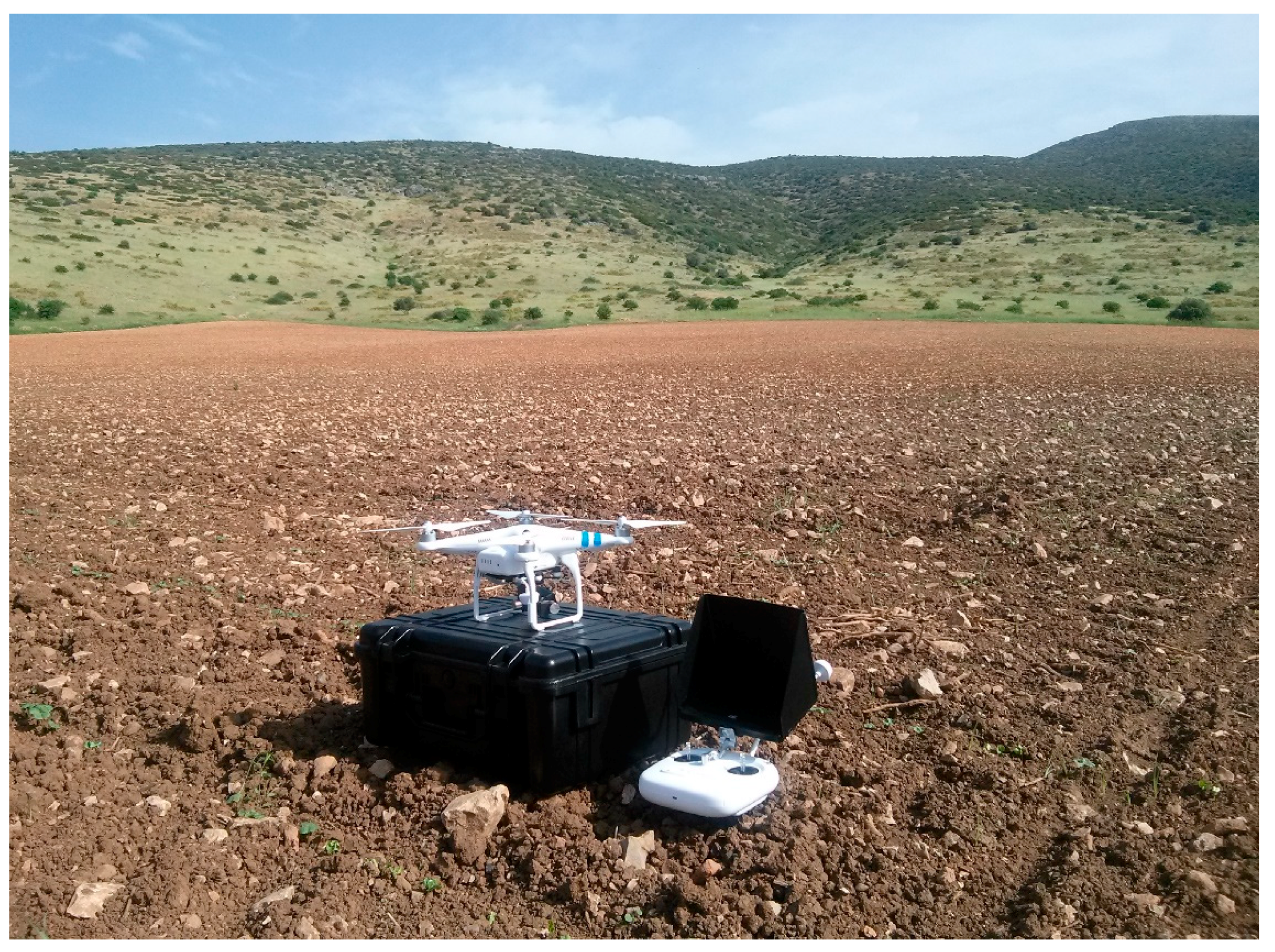
The unmanned aerial system (UAS) set before a flight mission in Field 2 (original photograph).
Figure 6.
The unmanned aerial system (UAS) set before a flight mission in Field 2 (original photograph).

Figure 7.
Steps of the analysis followed.

Figure 8.
Spatially interpolated maps by ordinary kriging of selected soil and plant properties in field 1 (left) and 2 (right).
Figure 8.
Spatially interpolated maps by ordinary kriging of selected soil and plant properties in field 1 (left) and 2 (right).


Figure 9.
Zones recognized by Fuzzy c-means algorithm in Field 1 concerning soil characteristics.

Figure 10.
Zones recognized by Fuzzy c-means algorithm in Field 2 concerning soil characteristics.

Figure 11.
Zones recognized by Fuzzy c-means algorithm in Field 1 concerning crop characteristics.

Figure 12.
Zones recognized by Fuzzy c-means algorithm in Field 2 concerning crop characteristics. Nevertheless, mean values of the measured crop parameters (Table 19) did not statistically differentiate among the two zones, with the exception of iron concentration (significance level p < 0.01), as similarly observed in Field 1. In both cases, despite the minimum variability observed between the two zones extracted per field, zoning—as achieved—may contribute and guide future plant sampling schemes.


Table 1.
Descriptive statistics of soil parameters regarding Field 1.
| Field 1 | Minimum | Maximum | Mean | Std. Deviation |
|---|---|---|---|---|
| Clay (%) | 26 | 50 | 36.9 | 6.5 |
| EC (mS/cm) | 0.7 | 1.2 | 0.9 | 0.1 |
| pH | 7.3 | 7.9 | 7.6 | 0.1 |
| Organic Matter (%) | 0.3 | 3.6 | 2.0 | 0.7 |
| CaCO3 (%) | 0.4 | 6.3 | 2.5 | 1.3 |
| Total nitrogen (mg/g) | 0.8 | 1.9 | 1.1 | 0.2 |
Table 2.
Descriptive statistics of soil parameters regarding Field 2.
| Field 2 | Minimum | Maximum | Mean | Std. Deviation |
|---|---|---|---|---|
| Clay (%) | 38 | 52 | 46.2 | 3.7 |
| EC (mS/cm) | 0.8 | 2.3 | 1.3 | 0.4 |
| pH | 7.1 | 7.7 | 7.4 | 0.2 |
| Organic Matter (%) | 0.4 | 6.7 | 4.1 | 1.0 |
| CaCO3 (%) | 1.2 | 17.0 | 5.5 | 4.2 |
| Total nitrogen (mg/g) | 0.3 | 4.1 | 1.6 | 0.6 |
Table 3.
Descriptive statistics of leaf nutrient content regarding Field 1.
| Field 1 | Minimum | Maximum | Mean | Std. Deviation |
|---|---|---|---|---|
| Total nitrogen (%) | 1.9 | 4.0 | 3.4 | 0.4 |
| Potassium (g/100 g) | 3.6 | 5.5 | 4.8 | 0.5 |
| Iron (ppm) | 33.0 | 78.0 | 50.3 | 9.9 |
| Copper (ppm) | 1.0 | 6.0 | 3.9 | 1.2 |
| Zinc (ppm) | 13.0 | 24.0 | 19.5 | 2.8 |
Table 4.
Descriptive statistics of leaves’ nutrient content regarding Field 2.
| Field 2 | Minimum | Maximum | Mean | Std. Deviation |
|---|---|---|---|---|
| Total nitrogen (%) | 3.3 | 4.3 | 3.7 | 0.2 |
| Potassium (g/100 g) | 3.7 | 5.7 | 4.9 | 0.6 |
| Iron (ppm) | 42.0 | 65.0 | 49.0 | 6.3 |
| Copper (ppm) | 2.0 | 6.0 | 4.8 | 0.9 |
| Zinc (ppm) | 25.0 | 32.0 | 28.2 | 2.0 |
Table 5.
Best fitted semivariogram models and model parameters for soil and plant parameter of the studying fields.
Table 5.
Best fitted semivariogram models and model parameters for soil and plant parameter of the studying fields.
| Parameter | Field | Model | Range (m) | Nugget (C0) | Partial sill (C) | Sill (C0+C) | Nugget/Sill |
|---|---|---|---|---|---|---|---|
| Clay | 1 | Pentaspherical | 371.66 | 2.01 | 80.71 | 82.72 | 0.02 |
| 2 | Pentaspherical | 283.40 | 5.28 | 15.52 | 20.80 | 0.25 | |
| EC | 1 | Spherical | 46.45 | 0.001 | 0.01 | 0.01 | 0.09 |
| 2 | Gaussian | 283.40 | 0.1 | 0.22 | 0.32 | 0.31 | |
| pH | 1 | Spherical | 57.79 | 0.01 | 0.01 | 0.02 | 0.50 |
| 2 | Spherical | 283.40 | 0.01 | 0.03 | 0.04 | 0.25 | |
| Organic Matter | 1 | Gaussian | 115.32 | 0.21 | 0.22 | 0.43 | 0.49 |
| 2 | Circular | 50.82 | 0.64 | 0.29 | 0.93 | 0.69 | |
| CaCO3 | 1 | Gaussian | 371.66 | 0.75 | 3.59 | 4.34 | 0.17 |
| 2 | Gaussian | 179.99 | 3.52 | 27.29 | 30.81 | 0.11 | |
| Total soil nitrogen | 1 | Pentaspherical | 46.45 | 0.001 | 0.04 | 0.04 | 0.02 |
| 2 | Exponential | 143.64 | 0.003 | 0.51 | 0.51 | 0.006 | |
| Total plant nitrogen | 1 | Exponential | 166.56 | 0.001 | 0.29 | 0.29 | 0.003 |
| 2 | Exponential | 51.09 | 0.02 | 0.05 | 0.07 | 0.29 | |
| Potassium | 1 | Pentaspherical | 87.32 | 0.001 | 0.21 | 0.21 | 0.005 |
| 2 | Exponential | 190.08 | 0.002 | 0.45 | 0.45 | 0.004 | |
| Iron | 1 | Circular | 56.11 | 14.99 | 93.87 | 108.86 | 0.14 |
| 2 | Circular | 70.12 | 3 | 42.02 | 45.02 | 0.07 | |
| Copper | 1 | Circular | 310.56 | 1.44 | 0.42 | 1.86 | 0.77 |
| 2 | Pentaspherical | 84.76 | 0.4 | 0.13 | 0.53 | 0.75 | |
| Zinc | 1 | Spherical | 95.18 | 2.66 | 6.58 | 9.24 | 0.29 |
| 2 | Spherical | 61.96 | 1.57 | 2.65 | 4.22 | 0.37 |
Table 6.
Correlation coefficients (r) between soil parameters, slope, and NIR in fields 1 and 2.
| Parameter | Field | NIR | Clay | EC | pH | Organic Matter | CaCO3 | Total Soil Nitrogen | Slope |
|---|---|---|---|---|---|---|---|---|---|
| NIR | 1 | 1 | |||||||
| 2 | 1 | ||||||||
| Clay | 1 | −0.581 ** | 1 | ||||||
| 2 | −0.007 | 1 | |||||||
| EC | 1 | 0.323 * | −0.596 ** | 1 | |||||
| 2 | −0.102 | 0.857 ** | 1 | ||||||
| pH | 1 | −0.054 | 0.236 * | −0.099 | 1 | ||||
| 2 | 0.359 * | −0.780 ** | −0.887 ** | 1 | |||||
| Organic Matter | 1 | −0.522 ** | 0.732 ** | −0.367 * | −0.003 | 1 | |||
| 2 | 0.429 ** | −0.081 | −0.386 * | 0.551 ** | 1 | ||||
| CaCO3 | 1 | −0.474 ** | 0.809 ** | −0.504 ** | 0.238 * | 0.831 ** | 1 | ||
| 2 | 0.692 ** | 0.033 | −0.225 * | 0.405 ** | 0.733 ** | 1 | |||
| Total soil nitrogen | 1 | −0.399 * | 0.713 ** | −0.595 ** | 0.349 * | 0.588 ** | 0.717 ** | 1 | |
| 2 | −0.333 * | 0.102 | −0.158 | −0.015 | 0.235 * | −0.043 | 1 | ||
| Slope | 2 | 0.378 * | 0.442 ** | 0.512 ** | −0.309 * | −0.019 | 0.276 * | −0.374 * | 1 |
** Correlation is significant at the 0.01 level. * Correlation is significant at the 0.05 level.
Table 7.
Results of principal component analysis (PCA) (soil) for Field 1.
| Principal Components | Eigenvalues | Variance (%) | Cumulative Variance (%) |
|---|---|---|---|
| 1 | 4.029 | 57.554 | 57.554 |
| 2 | 1.073 | 15.324 | 72.879 |
| 3 | 0.723 | 10.324 | 83.203 |
| 4 | 0.596 | 8.515 | 91.718 |
| 5 | 0.277 | 3.954 | 95.672 |
| 6 | 0.184 | 2.625 | 98.297 |
| 7 | 0.119 | 1.703 | 100.000 |
Table 8.
PCA (soil) loadings of the seven parameters concerning Field 1.
| Principal Components | NIR | Clay | EC | pH | OM | CaCO3 | Total Nitrogen |
|---|---|---|---|---|---|---|---|
| 1 | −0.703 | 0.896 | −0.644 | 0.041 | 0.882 | 0.886 | 0.758 |
| 2 | 0.125 | 0.211 | −0.214 | 0.947 | −0.103 | 0.206 | 0.442 |
Table 9.
Mean values of soil parameters per zone in Field 1.
| Zone | Clay (%) | EC (mS/cm) | pH | OM (%) | CaCO3 (%) | Total Nitrogen (%) |
|---|---|---|---|---|---|---|
| A | 42 | 0.89 | 7.67 | 2.4 | 3.5 | 1.2 |
| B | 34 | 0.97 | 7.63 | 1.8 | 2.0 | 1.0 |
Table 10.
Results of PCA (soil) for Field 2.
| Principal Components | Eigenvalues | Variance (%) | Cumulative Variance (%) |
|---|---|---|---|
| 1 | 3.312 | 41.396 | 41.396 |
| 2 | 2.346 | 29.323 | 70.719 |
| 3 | 1.323 | 16.543 | 87.262 |
| 4 | 0.387 | 4.832 | 92.094 |
| 5 | 0.321 | 4.017 | 96.111 |
| 6 | 0.187 | 2.343 | 98.454 |
| 7 | 0.072 | 0.896 | 99.350 |
| 8 | 0.052 | 0.650 | 100.000 |
Table 11.
PCA (soil) loadings of the eight parameters concerning Field 2.
| Principal Components | NIR | Clay | EC | pH | OM | CaCO3 | Total Nitrogen | Slope |
|---|---|---|---|---|---|---|---|---|
| 1 | −0.043 | 0.957 | 0.936 | −0.869 | −0.207 | −0.039 | 0.039 | 0.576 |
| 2 | 0.755 | 0.091 | −0.204 | 0.433 | 0.854 | 0.935 | 0.059 | 0.314 |
| 3 | −0.475 | 0.112 | −0.166 | −0.022 | 0.299 | −0.077 | 0.934 | −0.555 |
Table 12.
Mean values of soil parameters per zone in Field 2.
| Zone | Clay (%) | EC (mS/cm) | pH | OM (%) | CaCO3 (%) | Total Nitrogen (%) | Slope (%) |
|---|---|---|---|---|---|---|---|
| A | 44 | 1.12 | 7.48 | 3.9 | 3.1 | 1.6 | 6.5 |
| B | 47 | 1.26 | 7.45 | 4.2 | 6.8 | 1.4 | 9.1 |
Table 13.
Correlation coefficients (r) among plant parameters, slope, and NIR in Fields 1 and 2.
| Parameter | Field | NIR | Total Plant Nitrogen | Potassium | Iron | Copper | Zinc | Slope |
|---|---|---|---|---|---|---|---|---|
| NIR | 1 | 1 | ||||||
| 2 | 1 | |||||||
| Total plant nitrogen | 1 | 0.022 | 1 | |||||
| 2 | 0.126 | 1 | ||||||
| Potassium | 1 | −0.086 | 0.129 | 1 | ||||
| 2 | −0.147 | −0.500 ** | 1 | |||||
| Iron | 1 | −0.062 | −0.018 | 0.250 * | 1 | |||
| 2 | 0.071 | 0.507 ** | 0.091 | 1 | ||||
| Copper | 1 | −0.011 | 0.030 | 0.485 ** | 0.124 | 1 | ||
| 2 | −0.086 | −0.418 ** | 0.317 * | −0.305 * | 1 | |||
| Zinc | 1 | 0.066 | −0.328 * | −0.080 | −0.320 * | 0.212* | 1 | |
| 2 | −0.039 | −0.158 | 0.193 | 0.192 | 0.568 ** | 1 | ||
| Slope | 2 | 0.151 | 0.404 ** | −0.616 ** | 0.150 | −0.335 * | −0.174 | 1 |
** Correlation is significant at the 0.01 level. * Correlation is significant at the 0.05 level.
Table 14.
Results of PCA (plants) for Field 1.
| Principal Components | Eigenvalues | Variance (%) | Cumulative Variance (%) |
|---|---|---|---|
| 1 | 1.666 | 27.773 | 27.773 |
| 2 | 1.426 | 23.761 | 51.534 |
| 3 | 1.046 | 17.438 | 68.972 |
| 4 | 0.942 | 15.692 | 84.663 |
| 5 | 0.510 | 8.505 | 93.168 |
| 6 | 0.410 | 6.832 | 100.000 |
Table 15.
PCA (plants) loadings of the six parameters concerning Field 1.
| Principal Components | NIR | Potassium | Total Nitrogen | Iron | Copper | Zinc |
|---|---|---|---|---|---|---|
| 1 | 0.031 | 0.818 | 0.137 | 0.249 | 0.878 | 0.174 |
| 2 | 0.164 | 0.169 | 0.795 | 0.273 | −0.153 | −0.787 |
| 3 | 0.686 | −0.198 | 0.278 | −0.667 | 0.054 | 0.384 |
Table 16.
Mean values of crop parameters per zone in Field 1.
| Zone | Total Nitrogen (%) | Potassium (g/100 g) | Iron (ppm) | Copper (ppm) | Zinc (ppm) |
|---|---|---|---|---|---|
| A | 3.4 | 4.7 | 46.5 | 3.9 | 19.8 |
| B | 3.3 | 5.0 | 52.9 | 4.0 | 19.6 |
Table 17.
Results of PCA (plants) for Field 2.
| Principal Components | Eigenvalues | Variance (%) | Cumulative Variance (%) |
|---|---|---|---|
| 1 | 2.617 | 37.381 | 37.381 |
| 2 | 1.351 | 19.301 | 56.682 |
| 3 | 1.117 | 15.960 | 72.642 |
| 4 | 0.934 | 13.339 | 85.981 |
| 5 | 0.499 | 7.123 | 93.104 |
| 6 | 0.329 | 4.698 | 97.802 |
| 7 | 0.154 | 2.198 | 100.000 |
Table 18.
PCA (plants) loadings of the seven parameters concerning Field 2.
| Principal Components | NIR | Slope | Potassium | Total Nitrogen | Iron | Copper | Zinc |
|---|---|---|---|---|---|---|---|
| 1 | 0.433 | 0.791 | −0.871 | 0.493 | −0.041 | −0.159 | −0.034 |
| 2 | 0.115 | −0.202 | 0.236 | −0.243 | 0.062 | 0.807 | 0.918 |
| 3 | 0.054 | 0.149 | 0.039 | 0.664 | 0.962 | −0.389 | 0.175 |
Table 19.
Mean values of crop parameters per zone in Field 2.
| Zone | Total Nitrogen (%) | Potassium (g/100 g) | Iron (ppm) | Copper (ppm) | Zinc (ppm) |
|---|---|---|---|---|---|
| A | 3.6 | 5.0 | 47.4 | 4.9 | 19.8 |
| B | 3.8 | 4.7 | 52.3 | 4.6 | 19.6 |
Publisher’s Note: MDPI stays neutral with regard to jurisdictional claims in published maps and institutional affiliations. |
© 2021 by the authors. Licensee MDPI, Basel, Switzerland. This article is an open access article distributed under the terms and conditions of the Creative Commons Attribution (CC BY) license (http://creativecommons.org/licenses/by/4.0/).
Share and Cite
MDPI and ACS Style
Papadopoulos, A.V.; Kalivas, D.P. Assessing Soil and Crop Characteristics at Sub-Field Level Using Unmanned Aerial System and Geospatial Analysis. Sustainability 2021, 13, 2855. https://doi.org/10.3390/su13052855
AMA Style
Papadopoulos AV, Kalivas DP. Assessing Soil and Crop Characteristics at Sub-Field Level Using Unmanned Aerial System and Geospatial Analysis. Sustainability. 2021; 13(5):2855. https://doi.org/10.3390/su13052855
Chicago/Turabian StylePapadopoulos, Antonis V., and Dionissios P. Kalivas. 2021. "Assessing Soil and Crop Characteristics at Sub-Field Level Using Unmanned Aerial System and Geospatial Analysis" Sustainability 13, no. 5: 2855. https://doi.org/10.3390/su13052855
Note that from the first issue of 2016, this journal uses article numbers instead of page numbers. See further details here.