
A Spatial Improved-kNN-Based Flood Inundation Risk Framework for Urban Tourism under Two Rainfall Scenarios

1
School of Tourism and Public Management, Huzhou Vocational and Technical College, Huzhou 313000, China
2
College of Geospatial Information Science and Technology, Capital Normal University, Beijing 100048, China
3
International College, Huzhou University, Huzhou 313000, China
*
Author to whom correspondence should be addressed.
Sustainability 2021, 13(5), 2859; https://doi.org/10.3390/su13052859
Submission received: 1 February 2021
/
Revised: 28 February 2021
/
Accepted: 1 March 2021
/
Published: 6 March 2021
Abstract
:Urban tourism has been suffering socio-economic challenges from flood inundation risk (FIR) triggered by extraordinary rainfall under climate extremes. The evaluation of FIR is essential for mitigating economic losses, and even casualties. This study proposes an innovative spatial framework integrating improved k-nearest neighbor (kNN), remote sensing (RS), and geographic information system (GIS) to analyze FIR for tourism sites. Shanghai, China, was selected as a case study. Tempo-spatial factors, including climate, topography, drainage, vegetation, and soil, were selected to generate several flood-related gridded indicators as inputs into the evaluation framework. A likelihood of FIR was mapped to represent possible inundation for tourist sites under a moderate-heavy rainfall scenario and extreme rainfall scenario. The resultant map was verified by the maximum inundation extent merged by RS images and water bodies. The evaluation outcomes deliver the baseline and scientific information for urban planners and policymakers to take cost-effective measures for decreasing and evading the pressure of FIR on the sustainable development of urban tourism. The spatial improved-kNN-based framework provides an innovative, effective, and easy-to-use approach to evaluate the risk for the tourism industry under climate change.
1. Introduction
Flood inundation has been negatively affecting human society. It makes up a huge proportion of the reported natural disasters worldwide, and this quantity has been increasing over the last 30 years [1]. Especially in developing countries, fatalities and losses from flood inundation are disproportionally high [2]. For example, China recorded more than a thousand larger floods since 206 BC, and its flood damages account for a larger number of global flood losses (e.g., almost 10% in 1990–2017) [3], which is higher than other natural hazards. Besides, the worst flood events were observed globally, such as Australia and Thailand in 2011, central Europe in 2013, and India and Pakistan in 2014, which raises public interest in flood inundation [4,5]. Therefore, sufficient research in the field has been conducted to help people to understand, assess, and predict flood events and their impacts [6]. Looking ahead, continuing urban sprawl will locate on river flood-plains and coastal deltas due to population growth and migration (e.g., urban tourism), which will probably produce a substantial increase in flood inundation risk [7].
Urban tourism is an emerging and pollution-free sector. It brings various socio-economic benefits by providing employment and cultural exchange. For example, the figures in 2018 show that the number of foreign tourists in Shanghai, China, was about 6,859,000 [8], and brought around CNY 208 billion [9]. However, urban tourism also bears the negative brunt of extreme climates with destructive potentials. For example, tourism in Shanghai has suffered from annual losses of roughly CNY 22 million resulting from flood inundation [10]. Therefore, the evaluation of flood inundation risk (FIR) is vital for urban tourism to minimize or halt the adverse impacts of extreme weather on its sustainable development [11,12].
FIR is a comprehensive system combining natural hazards, vulnerability, and exposure [13]. Natural hazards refer to the frequency and intensity of hazards, and vulnerability denotes the susceptibility of the exposed elements to hazards, while exposure indicates population or assets located in flood-prone areas [11,14]. Many effective approaches have been used in FIR, such as expertise-based methods like analytic hierarchy process [15,16,17,18], probability-based evaluations like Bayesian networks [13,19], machine-learning-based approaches like neural networks [20,21,22,23,24], and hydrological and hydraulic models [25,26,27].
Besides, FIR embraces spatial and temporal features that have been explored by spatial technologies and methods [28], such as geographic information systems (GIS) [29] and remote sensing (RS) [30,31,32,33,34]. RS imagery as an important data resource has been broadly used in FIR owing to its wide coverage and rapid spatio-temporal updating. It can monitor and reflect dynamics on the earth’s surface [31]. Among the images, Landsat Thematic Mapper/Enhanced Thematic Mapper Plus (TM/ETM+) and Moderate Resolution Imaging Spectroradiometer are popular spatial products, since their advantages lie in higher temporal resolutions and being well-suited for larger areas.
However, in light of the authors’ reading, some of the technologies and methods are relatively comprehensive, which is beyond many people’s scope of knowledge and skills. Besides, these investigations require sophisticated algorithm structures and abundant computations in modeling [35]. Therefore, this study attempts to select and apply a relatively easy-to-use algorithm to explore FIR.
The most prevalent and simple machine learning method is k-nearest neighbors (kNN), because of its easier interpretation and low calculation time. It has been largely employed in the hydraulic model [36], the classification of missing data [37], as well as traffic prediction [38]. The previous investigations have demonstrated that the kNN model performs more robustly for flood forecasting accuracy during longer periods than other methods (e.g., Kalman filter) at the Huai River in East China [39]. Still, it is rarely coupled with spatial technologies in FIR for the urban tourism industry, based on relatively limited coverage in the literature.
Hence, this study proposes an innovative methodology and conducts the following tasks: (1) improves the kNN algorithm; (2) proposes a novel spatial model integrating the improved kNN algorithm with spatial technologies; (3) employs the integrated model into FIR evaluation for urban tourism; and (4) compares the evaluation results between the new model and the original kNN method.
2. Framework Development
2.1. Basic Principle of kNN
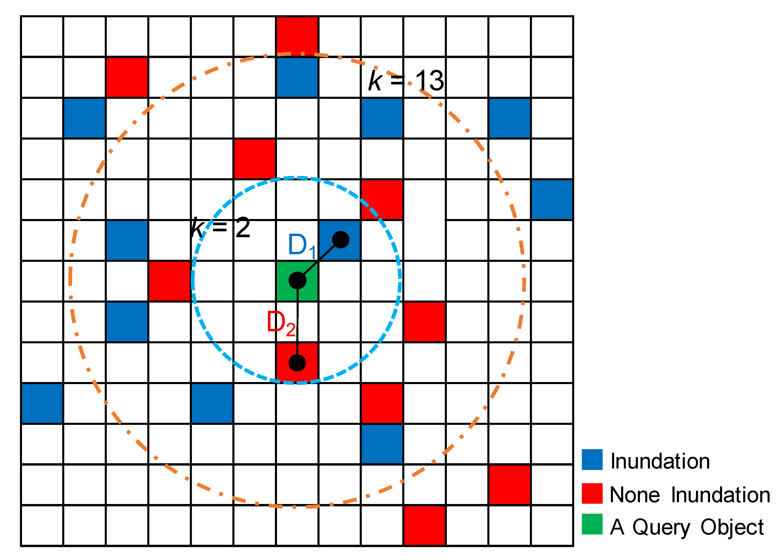
The principle of kNN refers to the feature of a query object being similar to the categories of the nearest objects [40]. It corresponds to Tobler’s first law of geography, which is the following: “All things are related, but nearby things are more related than distant things” [41]. In a kNN algorithm, two essential parameters determine the category of the query object. One is a value that determines the number of nearby neighbors. The other is a distance function that measures the similarity between the query object and the nearest objects. The commonly used function is Euclidean distance, which can be described as:
where and are query objects and nearby objects, respectively. and are the features of and .
Based on results calculated from Equation (1), the kNN algorithm will perform a vote, and the category of the nearest neighbor decides the class of the query object. However, the process of kNN inferring holds uncertainty, which can be further illustrated by Figure 1.
2.2. Improved Spatial kNN Algorithm
In Figure 1, objects fall into two categories, inundation or none inundation. A query object (in green) belongs to one of them. When equals 2, the query object belongs to inundation since the distance value of D1 is smaller than that of D2. However, when equals 13, the query object belongs to none inundation since the distance from the query object to objects in none inundation (in red) is less than the distance to objects in inundation (in blue). Hence, values determine the category of the query object. However, choosing an appropriate value is a major challenge in a kNN algorithm. Besides, the nearest object may be an invalid value or noise data, which brings the native impacts on the classification accuracy of kNN. Therefore, this study (1) calculates the total distance between the query object and nearby objects in inundation, and none inundation, respectively; and (2) uses probability to express the likelihood of inferred results to improve accuracy and diminish uncertainty in kNN. It can be expressed by the following formula:
where equates the total numbers of objects, while the numerator is the total distance between the query object to neighboring objects in inundation, and the denominator is the total distance between the query object to near inundated objects, and to nearby objects in none inundation.
2.3. Framework Conceptualization
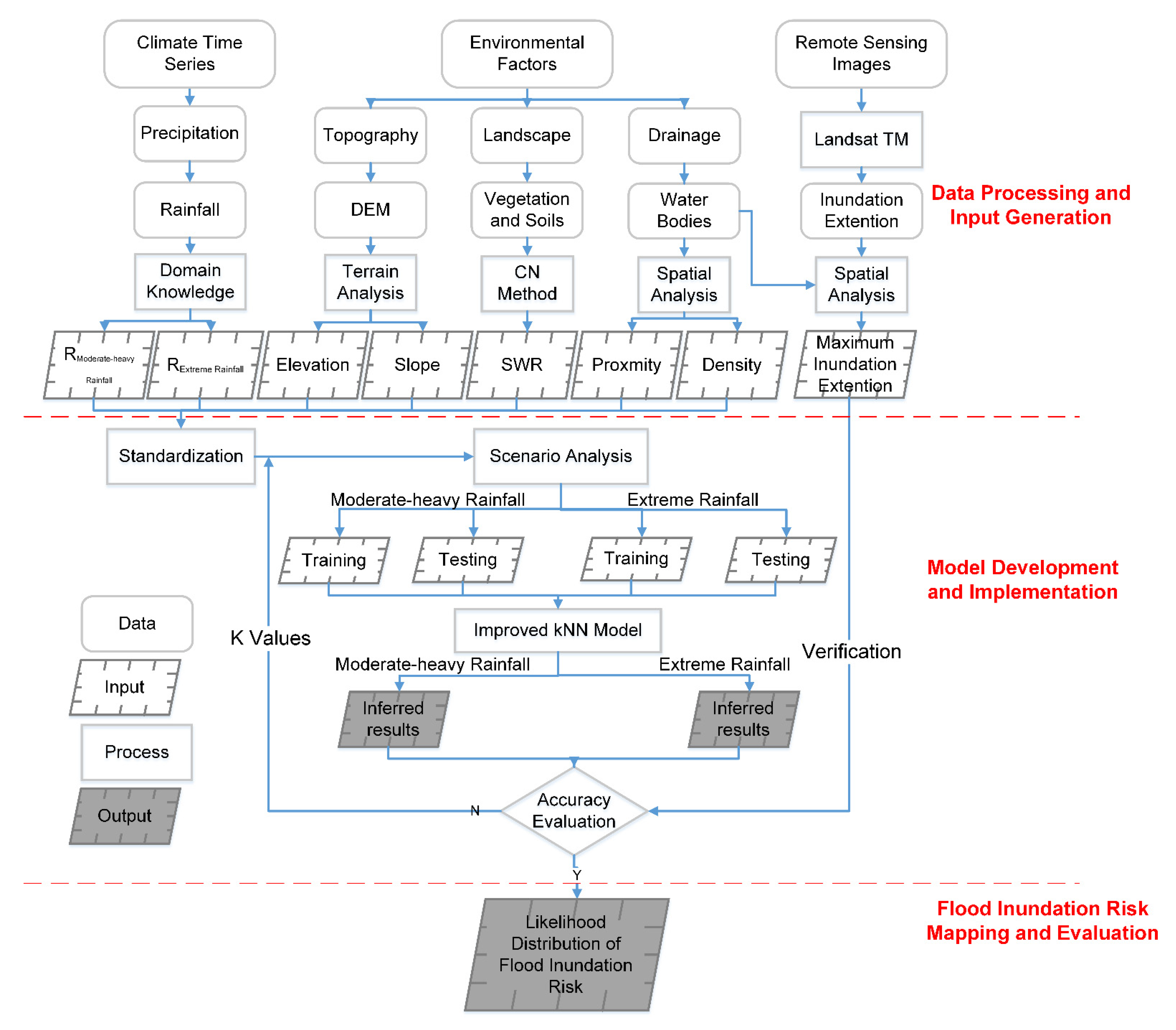
After a review of similar investigations, this study proposes a novel conceptualized framework integrating a spatial improved kNN method, RS, and GIS, based on gridded spatio-temporal data. The framework begins with spatial data acquisition, followed by model development and evaluation of FIR (Figure 2).
- Spatial data acquisition is the first module that includes the processing of spatial factors into the spatial improved kNN algorithm. The inundation extent, extracted from Landsat imagery, and observed water bodies are merged as the maximum inundation extent (MIE), which is employed as ground truth to verify spatial deduced results.
- Model development is the second module that contains the spatial improved kNN algorithm that is employed to infer the likelihood of FIR for query objects. The evaluation results are verified by MIE.
- Risk mapping and evaluation is the final module to produce and evaluate the spatial likelihood of FIR for tourism sites over a study area.
The model development and implementation is the core of the spatial framework, a detail which will be discussed.
2.4. Improved kNN Modeling and Implementation
Scenario-based methods are the commonly used way to explore the potential impact of FIR on populations or assets [42]. In this study, two scenarios, moderate-heavy rainfall scenario (MHRS) and extreme rainfall scenario (ERS), are designed to explore the impacts of rainfall on tourism sites. Following the first module, the evaluation indices are standardized from 1 to 4 to represent high to none risk. Based on values, training datasets are sampled randomly. The testing datasets, locating the corresponding positions of the training ones in MIE, are employed to verify the prediction results, which generates a confusion matrix. Four accurate indicators are generated from the matrix to evaluate the accuracy of the proposed model. They are overall accuracy (OA), kappa coefficient (Kappa), average producer’s accuracy (APA), and average user’s accuracy (AUA). The study compares the values of OA, Kappa, APA, and AUA with those in the previous iteration. The training datasets with the higher accurate values will be saved or, conversely, be omitted. After iterations, the most accurate and optimal training datasets will be employed to infer the likelihood of FIR cell by cell over the study area. These actions are processed in ArcGIS 10.2. Python language is employed to process the spatial data, and R scripting is used to infer the likelihood of FIR using the proposed model.
3. Case Study
3.1. Study Region
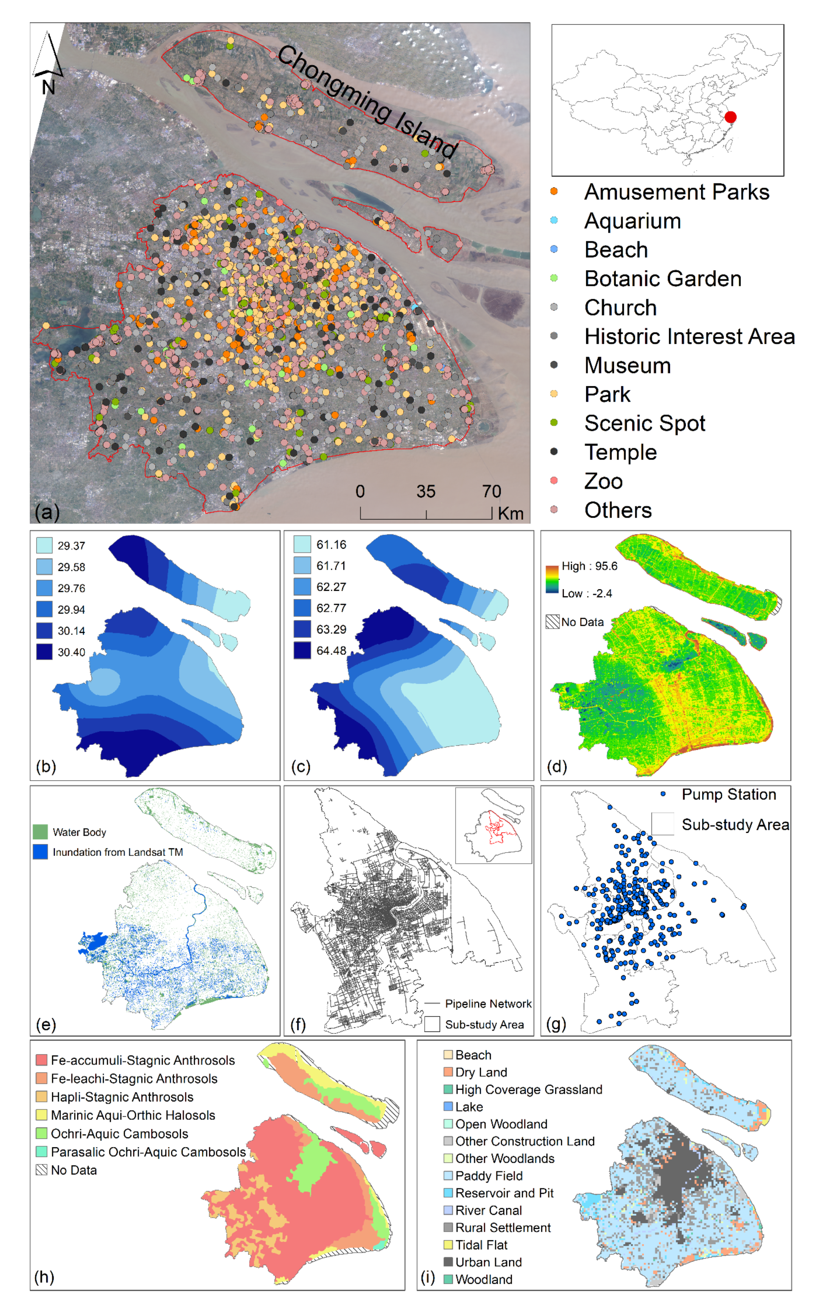
Shanghai is an internationally celebrated city and a tourism destination with a huge number of well-known attractions (Figure 3a), such as the Bund and Oriental Pearl. It has a population of more than 24 million [43,44]. The population density is about 4000 people per km2, which is larger than that of other cities in China. The terrestrial area of it is 6340 km2, which is surrounded by water on three sides: the Yangtze River Estuary up to the north; the East China Sea to the east; and Hangzhou Bay down to the south. The Huangpu River and the Suzhou Creek pass through the city. The whole city is situated in a flat and low-lying coastal region where the average elevation is about 4 m. The region is regarded as a climate with highly variable conditions based on historical records. It is covered by a northern subtropical monsoon climate with four characteristic seasons. The mean annual precipitation is about 1200 mm, approximately 70% of which occurs during the wet season (April to September). Besides, the city is almost hit by typhoons with a frequency of 1.5 times annually. Also, the land-use pattern has changed with urban sprawl, which changes rainfall-runoff. These facts present an urgent need for evaluating FIR for tourism sites in modern cities.
3.2. Data Collection and Processing
FIR is a complex system, and various natural-social indices make it happen [45]. In this study, rainfall was defined as a driving factor, tourism sites as a vulnerability, and other indicators as disaster-prone environments [15]. Based on domain knowledge, nine indices include rainfall from climate, elevation and slope from topography, proximity and density from drainage, and soil water retention (SWR) from soil interacting with land use and land cover change (LUCC) (Table 1, Figure 3b–i).
Rainfall (short or prolonged periods) has the potential to be the largest and most critical impact on FIR [15,46]. Because of the limitation of datasets, spatial points extracted from APHRODITE were used to interpolate using Kriging in ArcGIS, and generate two indicators, R20 and R50, for a moderate-heavy rainfall scenario (MHRS) and extreme rainfall scenario (ERS), respectively (Table 1) [42,47,48]. APHRODITE has been demonstrated to accurately feature the seasonal migration of rain-belts in China [49]. Rainfall decides the formation of flood inundation, but topography determines the redistribution of FIR, since low-lying areas are more easily inundated where drainage systems are needed to reduce the likelihood of FIR. In this study, three levels of drainage systems were defined based on the speed of drainage under flood annual recurrence intervals (ARIs) (Table 2).
Land use and land cover mutually determine the filter capacity of soil types, which derives CN values. CN is a comprehensive parameter reflecting the characteristics of the watershed before rainfall, which has to do with antecedent moisture condition (AMC), the soil hydrologic characteristics, and ground cover condition, all of which are referenced from the list published by the Soil Conservation Service (SCS, Table 3) [60]. AMC is a key parameter in calculating the SWR, but it was always omitted in previous studies. In this study, AMC was divided into three categories: drought (AMC I), normal (AMC II), and wet (AMC III). The levels of AMC depend on the distance to water bodies. The closer to water bodies, the more humid the soil is.
This study categorized all the soil types into four categories from group A to group D. Group A includes Fe-leachi-Stagnic Anthrosols, Fe-accumuli-Stagnic Anthrosols, and Parasalic Ochri-Aquic Cambosols. Group B embraces Hapli-Stagnic Anthrosols and Ochri-Aquic Cambosols. Group C includes Fe-accumuli-Stagnic Anthrosols, and Group D covers Marinic Aqui-Orthic Halosols and Ochri-Aquic Cambosols. Based on the CN method (Table 1), the potential maximum SWR at cell (SWRi) is parameterized as a function of a CN (CNi) value for each cell.
Remote sensing imagery provides rich spatio-temporal data for FIR, but it is easily obscured by clouds. This study merged the processed water inundation extent extracted from Landsat TM images and water bodies to obtain maximum inundation extent (MIE) because of the poor quality of RS imagery [61]. MIE in the southwestern area matches the pattern of inundation extent from images well, which demonstrates the merged MIE can meet the needs of the study. The merged MIE was selected as a surrogate for ground truth to validate the final FIR map.
Since the extracted indices have various measurement scales, all data were registered, projected, rasterized at 100 m resolution, and clipped to the study area in ArcGIS. It rescales them to make each of the various factors contribute relatively equally to the occurrence of FIR. The normal method of rescaling is min-max normalization that can be described as
where is rescaled values of , and and are the minimum values and maximum values of the original dataset .
The calculated indices were reclassified from high to low likelihood of FIR in this study (Figure 4).
4. Results and Discussion
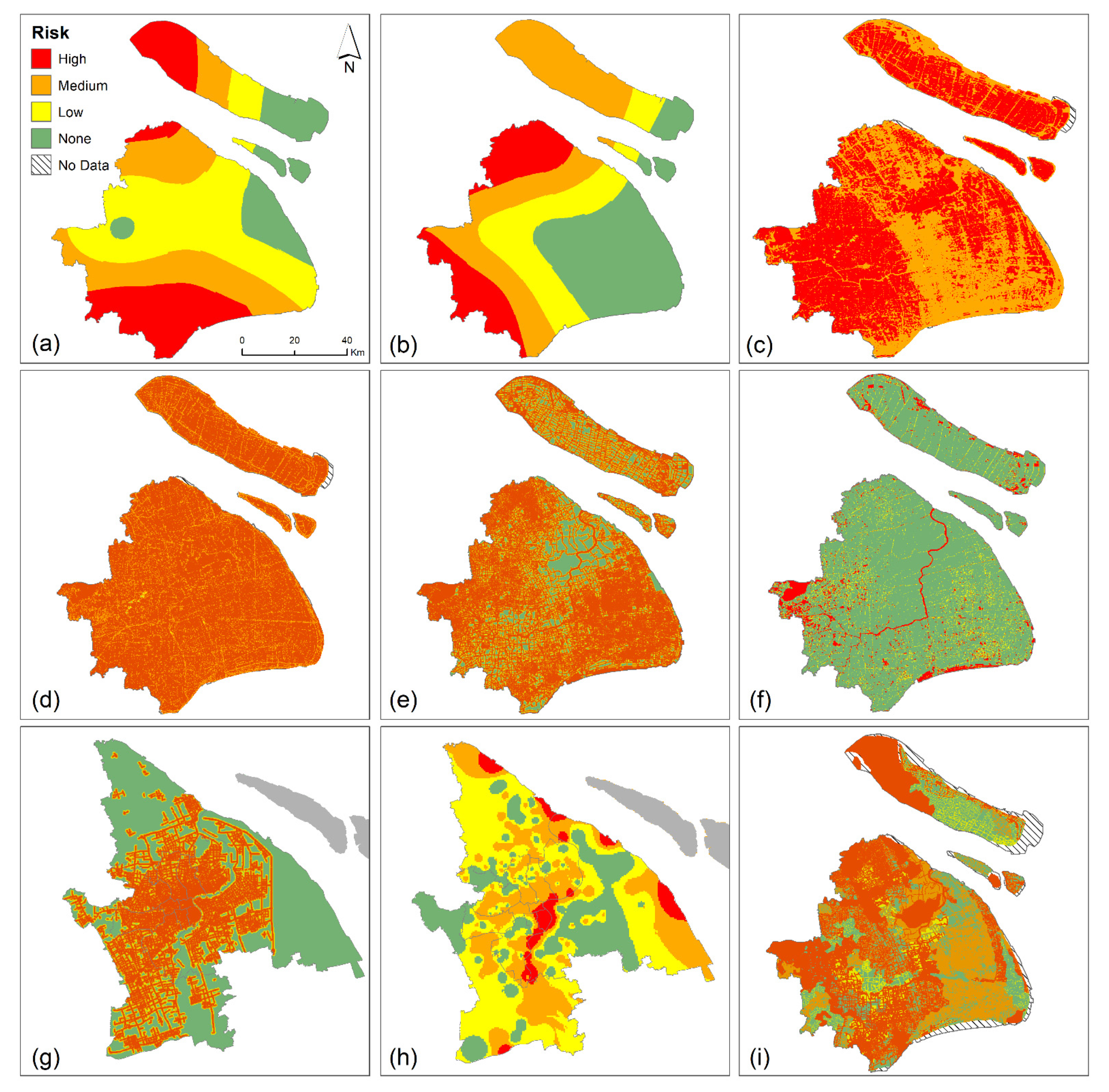
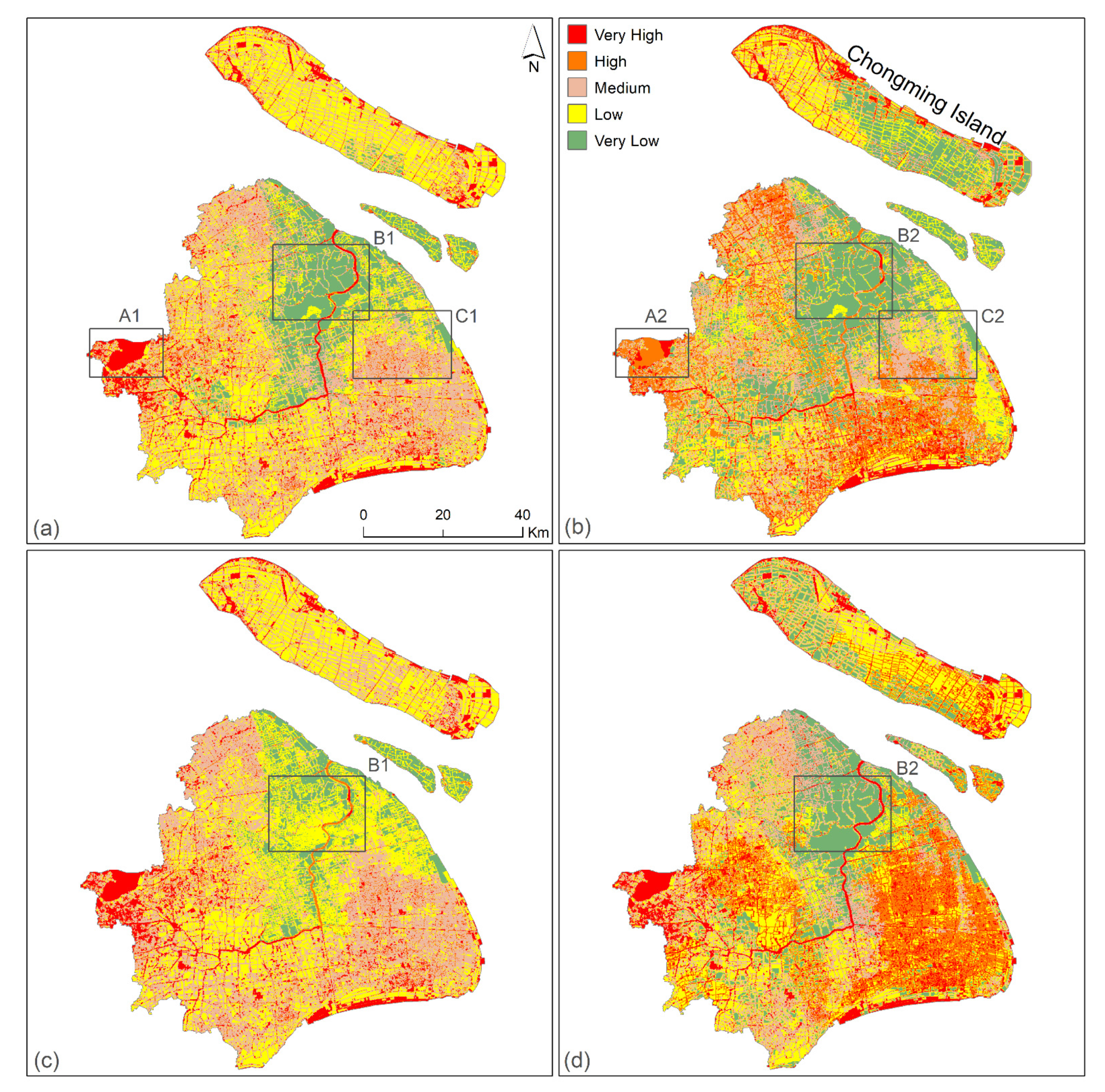
After calculation, FIR maps were derived as outputs from the proposed evaluation framework. The levels of spatial inferred results are divided into 5 levels: very high risk (red), high risk (orange), medium risk (medium sand), low (yellow), and very low (green) (Figure 5a,c) using Natural Breaks (Jenks) in ArcGIS because it picks the class breaks that maximize the differences between classes. Still, the classification method can be modified based on practical demands.
4.1. Result Validation
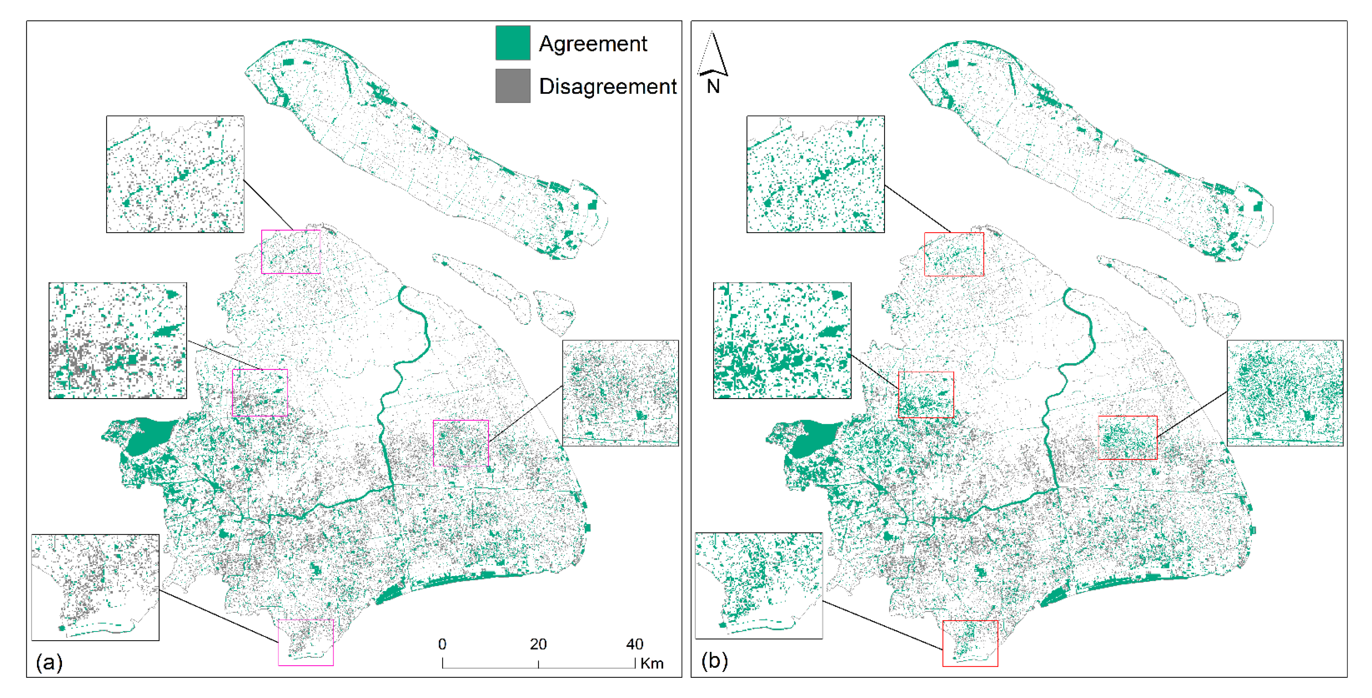
To validate the modeled results, the FIR maps in Figure 5a,c were further classified into 2 categories, inundation and none inundation, by using 50% as breakpoints. The breakpoint selected has considerable impacts on the FIR evaluation. Previous research reclassified their results based on domain knowledge. This study selected 50% as a threshold since we attempted to employ a cost-effective method to obtain relatively sound validation results. The likelihood of inundation is larger than 50%, while none inundation’s value is less than 50%. Two accurate comparisons were conducted between the evaluated results and MIE. The overlay calculations in MHRS (Figure 6a) and ERS (Figure 6b) present 54.19% and 62.87% of MIE, respectively. It should be noted that the inferred extents are smaller than MIE since some isolated cells cannot be identified as water areas or noise data.
4.2. Sensitivity and Uncertainty Analysis
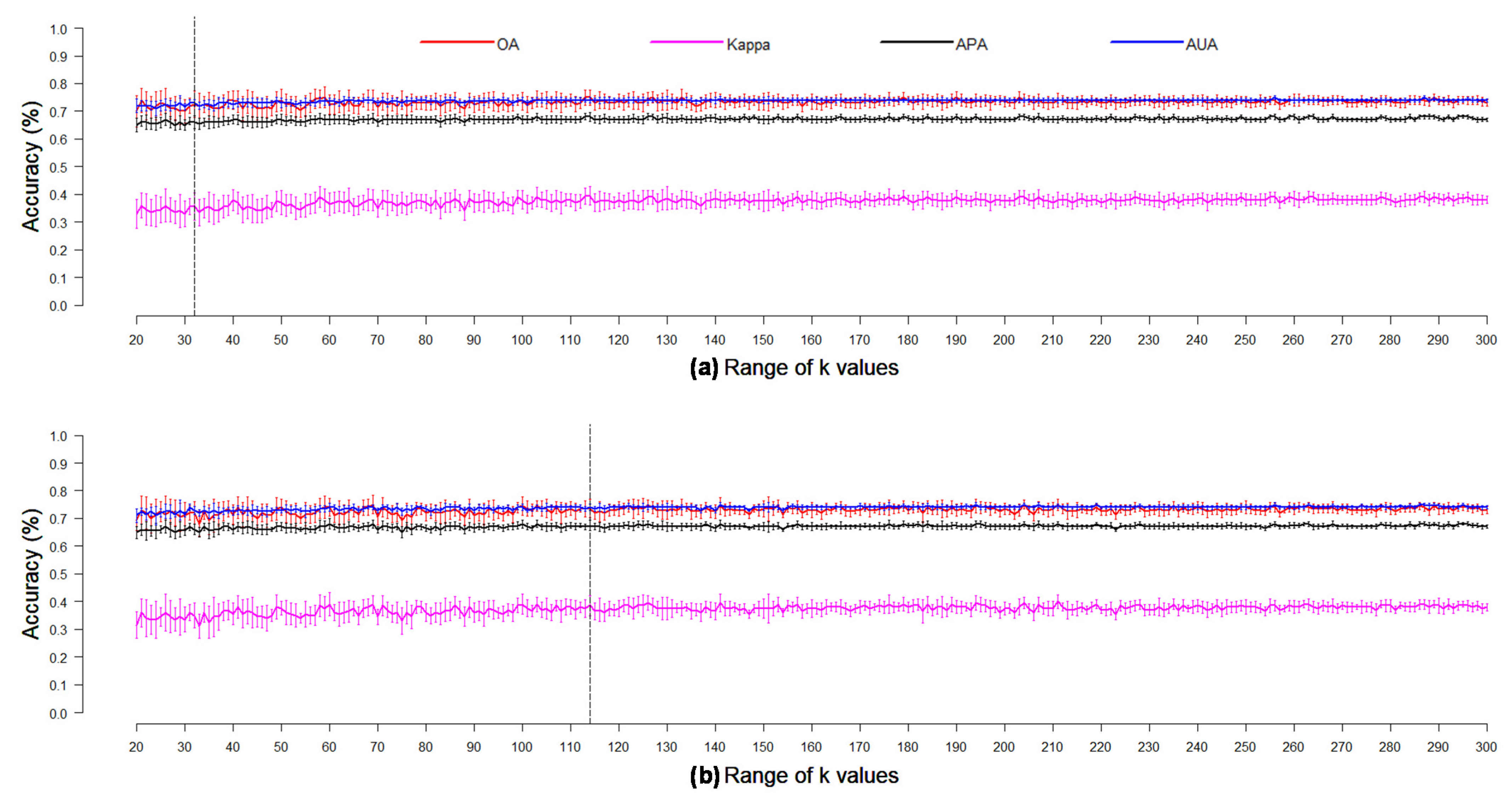
A sensitivity analysis is employed to explore the relationship between model inputs and outputs [62,63]. It is the key to understanding the parameters, uncertainty, and performance of a model. In this study, the pattern of FIR is altered with the change of rainfall in two scenarios, and values affect the accuracy of the model. Therefore, it is necessary to explore the relationship between the input values (rainfall and ) and the resultant evaluation using OA, Kappa, APA, and AUA to qualify the dependency between inputs and outputs (Figure 7).
In MHRS, the optimal accuracies of OA, Kappa, APA, and AUA equal 0.78, 0.42, 0.7, and 0.71, respectively (Figure 7a). However, their values in ERS increase to 0.8, 0.44, 0.71, and 0.74 (Figure 7b). This illustrates that the risk level rises with an increase in rainfall, which makes a huge contribution to FIR. Also, this study conducted around 16 million experiments to reveal the value range of the four accurate indicators in two rainfall scenarios. The experimental results show that their values maintain similar trends, which proves the improved kNN algorithm is stable in FIR. Besides, this study explored the changes of the four indicators in relation to values from 20 to 300. This demonstrated that the optimal accuracy can be produced when the values equal 32, 59, 114, and 139, which means the optimal accuracy is nothing to do with values in even numbers or odd numbers in this study.
Uncertainty broadly exists in flood risk evaluation [64], and it will decrease the accuracy of evaluation [65]. Landsat TM optical images as model inputs could miss flash rainfall events since study sites are frequently shielded by clouds during a flood period. It reduces the effectiveness of RS imagery to catch a fast-moving flood, and escalates uncertainty with the expansion of study areas [66]. Moreover, the uncertainty comes from the method of classification in the assessment. There are various methods in the classification of evaluation, such as natural breaks and standard deviation, each of which will produce dissimilar results. However, the conclusive evaluation is an uncertain result instead of the accumulation of all associated uncertainties in flood risk analysis [67]. For this reason, scenarios may be the “best” ways to identify the “best” solution in FIR prediction or prevention [68].
4.3. Comparison between Improved kNN and kNN
From the visualization in Figure 5, the distribution of FIR in MHRS (a) and ERS (c) is right for the actual situation, compared with the evaluation results in MHRS (b) and ERS (d) using the original kNN. The main study area (Figure 5a,c) is covered by the low-to-medium level of FIR, since the area has facilities that are well equipped against flood inundation. In particular, the sub-study area is mainly situated in very low flood risk, since it has a high density of pipeline networks (Figure 3f) and pump stations (Figure 3g). These play an important role in lessening the level of FIR under the two scenarios.
Besides, the color gradients at a different FIR level in Figure 5a,c are smooth and natural, which matches the real spatial features of FIR transformation. Concretely, water bodies were located in the very high areas of FIR in Figure 5aA1, which is sound. Nevertheless, they are covered by a medium level in FIR in Figure 5bA2. Moreover, the evaluation results in B1 (Figure 5a,c) show that the level of FIR increase with the rise of rainfall using the improved kNN method. However, B2 in Figure 5b,d cannot reflect this trend, or even show decreases in FIR. Furthermore, the evaluation results from the original kNN are heavily affected by specific factors. For example, C2 in Figure 5b is mainly influenced by precipitation (Figure 3b), and Chongming Island is mainly affected by SWR (Figure 4i). For classification precision, the evaluation accuracies of OA, Kappa, APA, and AUA are only 0.61, 0.25, 0.59, and 0.61 in MHRS (Figure 5b), and 0.63, 0.27, 0.6, and 0.61 in ERS (Figure 5d) using the original kNN method.
4.4. Distribution of FIR
FIR is interactively influenced and controlled by the multiple input indices. Figure 5a,c show that the areas above high FIR mainly follow the spatial pattern of two indices, proximity (Figure 4e) and density (Figure 4f). They are extracted from water bodies (Figure 3e), pipeline networks (Figure 4g), and pump stations (Figure 4h). When the volume of runoff water exceeds the conveying capacity of water channels, it easily inundates the areas surrounding the water bodies [35,69]. Rainfall (Figure 4a,b) contributes to the north area and the west-south area. Besides, elevation (Figure 4c), slope (Figure 4d), and SWR (Figure 4i) mutually decide the redistribution of FIR in these areas because of poor soil porousness and steepness, which make rainfall stay on the earth’s surface.
In the sub-study area, the risk above medium level is mainly located at the tributaries of the Huangpu River and the confluence of other rivers, since these areas are fed by excessive waters from surrounding areas [70,71]. Moreover, the study area is covered by impervious surfaces that are not good for rainfall infiltration naturally [72]. Therefore, well-performing drainage systems play an important role in declining the likelihood of FIR. Figure 5a,c illustrate that the level of FIR in the sub-study area is relatively lower than that in other areas.
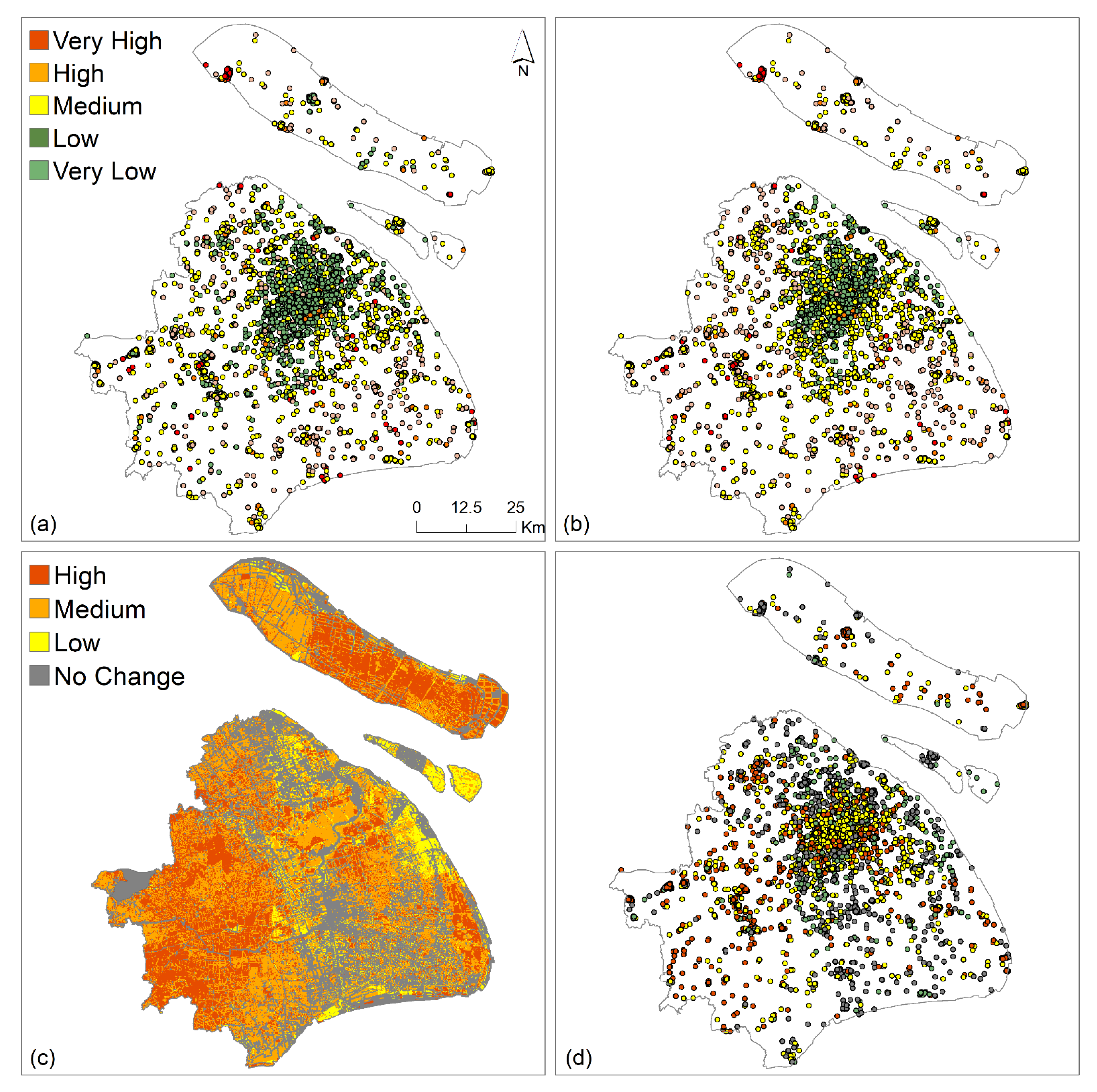
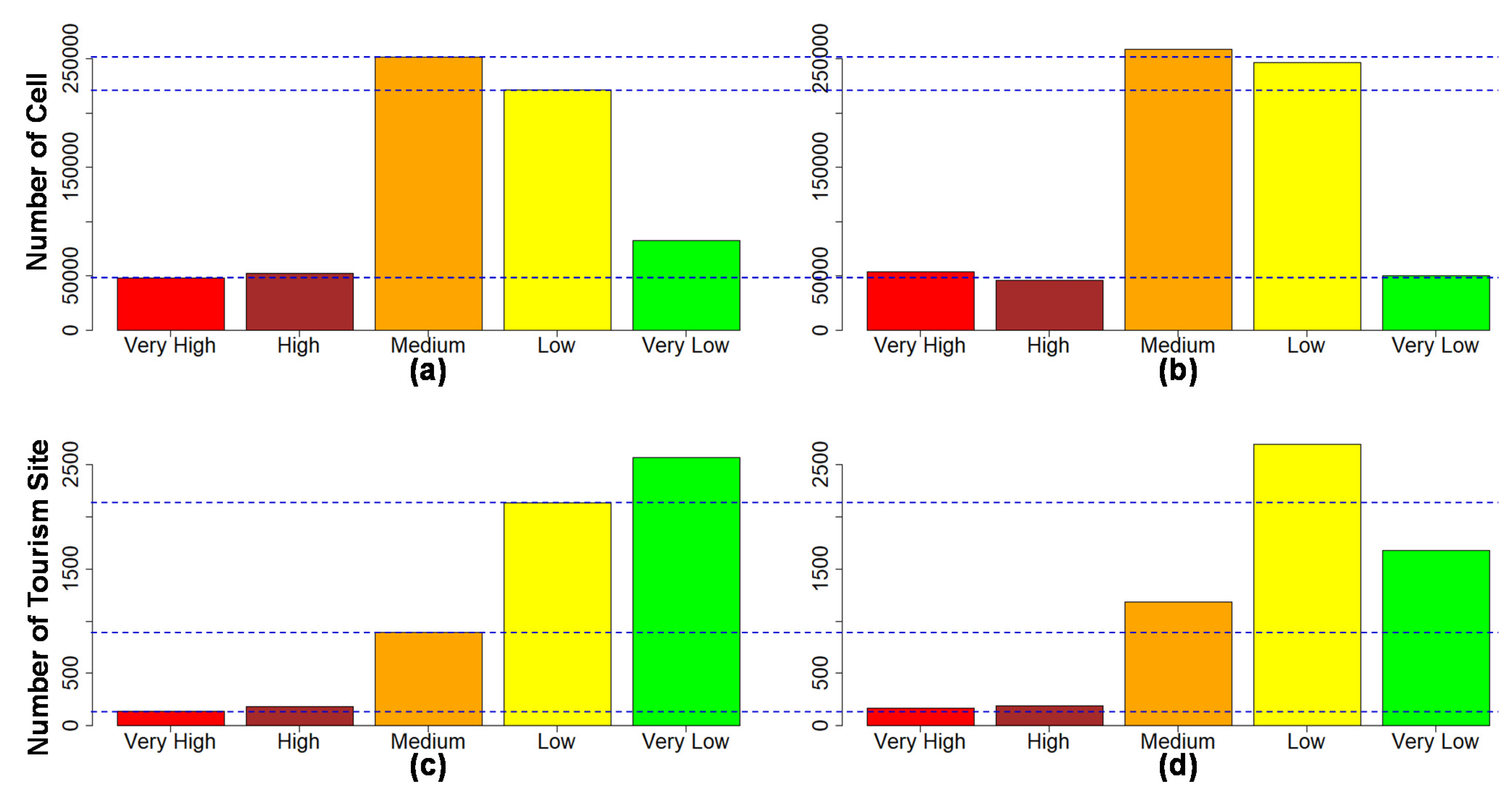
The statistics for FIR categories were conducted for the study area and tourism sites under the two scenarios (Figure 8a,b). MHRS (Figure 5a and Figure 9a) shows that about 7.3% of the total area is classified as very high risk (about 47,850 cells, about 478.50 km2), high risk accounts for 7.98% (about 522.85 km2), medium risk covers 38.39% (about 2515.34 km2), and low and very low risk occupy 33.73% (about 2210.09 km2) and 12.61% (about 826.13 km2), respectively. The numbers of tourism sites from very high to very low risk are 134, 178, 892, 2137, and 2571, respectively (Figure 8a and Figure 9c).
In ERS (Figure 5c and Figure 9b), the areas of very high, medium, and low risk increase. Areas classified as very high risk represent 8.2% of the total area (about 537.28 km2), high risk is about 7.03% (about 460.37 km2), medium risk is about 39.49% (about 2587.57 km2), and low and very low are about 37.60% (about 2463.97 km2) and 7.69% (about 503.72 km2), respectively. The numbers of tourism sites from very high risk to very low risk are 164, 190, 1188, 2691, and 1676, respectively (Figure 8b and Figure 9d).
To illustrate the hotspots in FIR changes from MHRS to ERS, the calculated MHRS-ERS growth rate was classified into three levels, high, medium, and low, using natural breakpoints of 2.20% and 7.00% (Figure 8c). The percentages of very high, medium, and low risk increase by 0.9% (about 58.78 km2), 1.10% (about 72.23 km2), and 3.87% (about 253.88 km2), respectively (Figure 9a,b). The increasing areas in high risk are mainly located in the west, central, and east-south areas of Chongming Island, because these areas have a high density of water bodies and lower elevation.
With the increase of FIR from MHRS to ERS, 30 tourism sites rise to very high risk, with 12 sites becoming high risk, 296 sites becoming medium risks, and 557 sites becoming low risk (Figure 8d and Figure 9c,d). Among these medium-and-above sites, historic interests occupy the highest percentage, followed by amusement parks, scenic spots, and churches. The vulnerability of tourism sites is projected to increase along river channels with the increase of rainfall due to an increase in the volume of fast-flowing surface water into rivers.
5. Conclusions
This study proposes a spatial innovative framework to evaluate the likelihood of flood inundation risk (FIR) integrating improved k-nearest neighbors (kNN), RS, and GIS. The improved kNN algorithm was applied to deduce the likelihood of FIR based on multiple sources of spatial flood-related factors. RS was used to extract a maximum inundation extent for data sampling and result validation. GIS was employed to derive input indices via processing a variety of data at multi-temporal, multi-spatial resolutions. The spatial framework illustrates that the methodology can derive sound results. The results show that (1) the improved kNN algorithm is right for FIR; and (2) likelihood can better indicate uncertainty using the kNN algorithm in FIR. The spatial framework was programmed and repeatable. The methodology is not limited by the number of input indices. If the inputs of the framework are changed, the evaluation results will be changed and generated accordingly. Therefore, the approach can be used as a feasible methodology not only in FIR, but also in other likelihood-related hazard investigations. The practice provides the baseline information for urban planners or decision-makers to construct cost-effective measures that lessen and avoid the pressure of FIR on the tourism industry.
However, good-quality RS images are vital for FIR evaluation, but they are hard to obtain during severe rainfall or large flood events, which may result in missing out on flash rainfall events. This study had to employ the processed inundation extent from Landsat TM, but its extent affects the evaluation accuracy of the spatial framework. Besides, the resolution of rainfall is coarse, which also determines the formation and spatial distribution of FIR. Furthermore, this study does not consider hydrological factors such as rainfall duration and speed. As a further step, the study plans to conduct sensitivity analysis to explore the relationship between selected breakpoints in result validation and evaluation accuracy, and we will investigate more parameters for delivering more robust evaluation results with the least uncertainty.
Author Contributions
Conceptualization, R.L. and S.L.; methodology, R.L.; software, N.T.; validation, R.L., S.L. and N.T.; formal analysis, S.L.; investigation, S.L.; resources, S.L.; data curation, N.T.; writing—original draft preparation, S.L.; writing—review and editing, R.L.; visualization, N.T.; supervision, R.L.; project administration, S.L.; funding acquisition, S.L. All authors have read and agreed to the published version of the manuscript.
Funding
The study was funded by Research on Practical Teaching Mode of Tourism Major in Higher Vocational Education Based on CBE Mode (FG2019131), Research on the Design and Application of Smart Classroom Mode under the Background of “Internet + Education” (186140055), and Seeing Beautiful China in Huzhou: Evolution and Development of Villages in Tourist Attractions in Huzhou (20hzghy026). The anonymous reviewers are acknowledged for their valuable comments.
Institutional Review Board Statement
No applicable.
Informed Consent Statement
No applicable.
Data Availability Statement
No applicable.
Acknowledgments
The authors also want to appreciate Chongxiao Wan for providing the data for this study and Siyi Yu for some technical support.
Conflicts of Interest
The authors declare no conflict of interest.
References
- Rougier, J.; Sparks, S.; Hill, L. Risk and Uncertainty Assessment for Natural Hazards; Cambridge University Press: Cambridge, UK, 2013. [Google Scholar]
- Hawker, L.; Neal, J.; Tellman, B.; Liang, J.; Schumann, G.; Doyle, C.; Sullivan, J.A.; Savage, J.; Tshimanga, R. Comparing earth observation and inundation models to map flood hazards. Environ. Res. Lett. 2020, 15, 124032. [Google Scholar] [CrossRef]
- Kundzewicz, Z.W.; Su, B.; Wang, Y.; Xia, J.; Huang, J.; Jiang, T. Flood risk and its reduction in China. Adv. Water Resour. 2019, 130, 37–45. [Google Scholar] [CrossRef]
- Sampson, C.C.; Smith, A.M.; Bates, P.D.; Neal, J.C.; Alfieri, L.; Freer, J.E. A high-resolution global flood hazard model. Water Resour. Res. 2015, 51, 7358–7381. [Google Scholar] [CrossRef] [PubMed] [Green Version]
- Rajib, A.; Liu, Z.; Merwade, V.; Tavakoly, A.A.; Follum, M.L. Towards a large-scale locally relevant flood inundation modeling framework using SWAT and LISFLOOD-FP. J. Hydrol. 2020, 581, 124406. [Google Scholar] [CrossRef]
- Teng, J.; Jakeman, A.J.; Vaze, J.; Croke, B.F.W.; Dutta, D.; Kim, S. Flood inundation modelling: A review of methods, recent advances and uncertainty analysis. Environ. Model. Softw. 2017, 90, 201–216. [Google Scholar] [CrossRef]
- Darabi, H.; Choubin, B.; Rahmati, O.; Torabi Haghighi, A.; Pradhan, B.; Kløve, B. Urban flood risk mapping using the GARP and QUEST models: A comparative study of machine learning techniques. J. Hydrol. 2019, 569, 142–154. [Google Scholar] [CrossRef]
- Mou, N.; Yuan, R.; Yang, T.; Zhang, H.; Tang, J.; Makkonen, T. Exploring spatio-temporal changes of city inbound tourism flow: The case of Shanghai, China. Tour. Manag. 2020, 76, 103955. [Google Scholar] [CrossRef]
- Shanghai Bureau of Statistics. Available online: http://tjj.sh.gov.cn/tjnj/nj19.htm?d1=2019tjnj/C0408.htm (accessed on 12 December 2020).
- Quan, R. Rainstorm waterlogging risk assessment in central urban area of Shanghai based on multiple scenario simulation. Nat. Hazards 2014, 73, 1569–1585. [Google Scholar] [CrossRef]
- Muis, S.; Guneralp, B.; Jongman, B.; Aerts, J.C.; Ward, P.J. Flood risk and adaptation strategies under climate change and urban expansion: A probabilistic analysis using global data. Sci. Total Environ. 2015, 538, 445–457. [Google Scholar] [CrossRef]
- Luu, C.; Tran, H.X.; Pham, B.T.; Al-Ansari, N.; Tran, T.Q.; Duong, N.Q.; Dao, N.H.; Nguyen, L.P.; Nguyen, H.D.; Thu Ta, H.; et al. Framework of spatial flood risk assessment for a case study in Quang Binh province, Vietnam. Sustainability 2020, 12, 3058. [Google Scholar] [CrossRef] [Green Version]
- Liu, R.; Chen, Y.; Wu, J.; Gao, L.; Barrett, D.; Xu, T.; Li, X.; Li, L.; Huang, C.; Yu, J. Integrating entropy-based Naive Bayes and GIS for spatial evaluation of flood hazard. Risk Anal. 2017, 37, 756–773. [Google Scholar] [CrossRef]
- Suzuki, T. Building up a common recognition of city development in the southern part of Kofu basin under the initiative of knowledge brokers with the cooperation of experts. Sustainability 2020, 12, 6316. [Google Scholar] [CrossRef]
- Chen, Y.; Liu, R.; Barrett, D.; Gao, L.; Zhou, M.; Renzullo, L.; Emelyanova, I. A spatial assessment framework for evaluating flood risk under extreme climates. Sci. Total Environ. 2015, 538, 512–523. [Google Scholar] [CrossRef] [PubMed]
- Chakraborty, S.; Mukhopadhyay, S. Assessing flood risk using analytical hierarchy process (AHP) and geographical information system (GIS): Application in Coochbehar district of West Bengal, India. Nat. Hazards 2019, 99, 247–274. [Google Scholar] [CrossRef]
- Costache, R.; Dieu Tien, B. Identification of areas prone to flash-flood phenomena using multiple-criteria decision-making, bivariate statistics, machine learning and their ensembles. Sci. Total Environ. 2020, 712, 136492. [Google Scholar] [CrossRef] [PubMed]
- Lin, K.; Chen, H.; Xu, C.; Yan, P.; Lan, T.; Liu, Z.; Dong, C. Assessment of flash flood risk based on improved analytic hierarchy process method and integrated maximum likelihood clustering algorithm. J. Hydrol. 2020, 584, 124696. [Google Scholar] [CrossRef]
- Liu, R.; Chen, Y.; Wu, J.; Gao, L.; Barrett, D.; Xu, T.; Li, L.; Huang, C.; Yu, J. Assessing spatial likelihood of flooding hazard using naïve Bayes and GIS: A case study in Bowen Basin, Australia. Stoch. Environ. Res. Risk Assess. 2015, 30, 1575–1590. [Google Scholar] [CrossRef]
- Li, L.; Chen, Y.; Xu, T.; Liu, R.; Shi, K.; Huang, C. Super-resolution mapping of wetland inundation from remote sensing imagery based on integration of back-propagation neural network and genetic algorithm. Remote Sens. Environ. 2015, 164, 142–154. [Google Scholar] [CrossRef]
- Li, L.; Chen, Y.; Yu, X.; Liu, R.; Huang, C. Sub-pixel flood inundation mapping from multispectral remotely sensed images based on discrete particle swarm optimization. Isprs J. Photogramm. Remote Sens. 2015, 101, 10–21. [Google Scholar] [CrossRef]
- Sajjad, M.; Lin, N.; Chan, J.C.L. Spatial heterogeneities of current and future hurricane flood risk along the US Atlantic and Gulf coasts. Sci. Total Environ. 2020, 713. [Google Scholar] [CrossRef]
- Schmidt, L.; Hesse, F.; Attinger, S.; Kumar, R. Challenges in applying machine learning models for hydrological Inference: A case study for flooding events across Germany. Water Resour. Res. 2020, 56, 5. [Google Scholar] [CrossRef]
- Wagenaar, D.; Curran, A.; Balbi, M.; Bhardwaj, A.; Soden, R.; Hartato, E.; Sarica, G.M.; Ruangpan, L.; Molinario, G.; Lallemant, D. Invited perspectives: How machine learning will change flood risk and impact assessment. Nat. Hazards Earth Syst. Sci. 2020, 20, 1149–1161. [Google Scholar] [CrossRef]
- Jamali, B.; Bach, P.M.; Deletic, A. Rainwater harvesting for urban flood management—An integrated modelling framework. Water Res. 2020, 171, 115372. [Google Scholar] [CrossRef]
- Nigussie, T.A.; Altunkaynak, A. Modeling the effect of urbanization on flood risk in Ayamama Watershed, Istanbul, Turkey, using the MIKE 21 FM model. Nat. Hazards 2019, 99, 1031–1047. [Google Scholar] [CrossRef]
- Jahandideh-Tehrani, M.; Helfer, F.; Zhang, H.; Jenkins, G.; Yu, Y.Y. Hydrodynamic modelling of a flood-prone tidal river using the 1D model MIKE HYDRO River: Calibration and sensitivity analysis. Environ. Monit. Assess. 2020, 192, 1–18. [Google Scholar] [CrossRef]
- Liu, Y.; De Smedt, F. Flood modeling for complex terrain using GIS and remote sensed information. Water Resour. Manag. 2005, 19, 605–624. [Google Scholar] [CrossRef]
- Swain, K.C.; Singha, C.; Nayak, L. Flood susceptibility mapping through the GIS-AHP technique using the cloud. ISPRS Int. J. Geo-Inf. 2020, 9, 720. [Google Scholar] [CrossRef]
- Merwade, V.; Cook, A.; Coonrod, J. GIS techniques for creating river terrain models for hydrodynamic modeling and flood inundation mapping. Environ. Model. Softw. 2008, 23, 1300–1311. [Google Scholar] [CrossRef]
- Chen, Y.; Huang, C.; Ticehurst, C.; Merrin, L.; Thew, P. An evaluation of MODIS daily and 8-day composite products for floodplain and wetland inundation mapping. Wetlands 2013, 33, 823–835. [Google Scholar] [CrossRef]
- Chen, Y.; Wang, B.; Pollino, C.A.; Cuddy, S.M.; Merrin, L.E.; Huang, C. Estimate of flood inundation and retention on wetlands using remote sensing and GIS. Ecohydrology 2014, 7, 1412–1420. [Google Scholar] [CrossRef]
- Huang, C.; Chen, Y.; Wu, J. Mapping spatio-temporal flood inundation dynamics at large river basin scale using time-series flow data and MODIS imagery. Int. J. Appl. Earth Obs. Geoinf. 2014, 26, 350–362. [Google Scholar] [CrossRef]
- Ticehurst, C.; Guerschman, J.; Chen, Y. The strengths and limitations in using the daily MODIS open water likelihood algorithm for identifying flood events. Remote Sens. 2014, 6, 11791–11809. [Google Scholar] [CrossRef] [Green Version]
- Darabi, H.; Haghighi, A.T.; Mohamadi, M.A.; Rashidpour, M.; Ziegler, A.D.; Hekmatzadeh, A.A.; Klove, B. Urban flood risk mapping using data-driven geospatial techniques for a flood-prone case area in Iran. Hydrol. Res. 2020, 51, 127–142. [Google Scholar] [CrossRef] [Green Version]
- Liu, K.; Li, Z.; Yao, C.; Chen, J.; Zhang, K.; Saifullah, M. Coupling the k-nearest neighbor procedure with the Kalman filter for real-time updating of the hydraulic model in flood forecasting. Int. J. Sediment Res. 2016, 31, 149–158. [Google Scholar] [CrossRef]
- Ma, Z.; Tian, H.; Liu, Z.; Zhang, Z. A new incomplete pattern belief classification method with multiple estimations based on KNN. Appl. Soft Comput. 2020, 90, 106175. [Google Scholar] [CrossRef]
- Xu, D.; Wang, Y.; Peng, P.; Beilun, S.; Deng, Z.; Guo, H. Real-time road traffic state prediction based on kernel-KNN. Transp. A Transp. Sci. 2018, 16, 104–118. [Google Scholar] [CrossRef]
- Liu, K.; Yao, C.; Chen, J.; Li, Z.; Li, Q.; Sun, L. Comparison of three updating models for real time forecasting: A case study of flood forecasting at the middle reaches of the Huai River in East China. Stoch. Environ. Res. Risk Assess. 2016, 31, 1471–1484. [Google Scholar] [CrossRef]
- Huang, C.; Chen, Y.; Wu, J. DEM-based modification of pixel-swapping algorithm for enhancing floodplain inundation mapping. Int. J. Remote Sens. 2013, 35, 365–381. [Google Scholar] [CrossRef]
- Tobler, W.R. A computer movie simulating urban growth in the detroit region. Econ. Geogr. 1970, 46, 234–240. [Google Scholar] [CrossRef]
- Chu, H.; Yu, J.; Wen, J.; Yi, M.; Chen, Y. Emergency evacuation simulation and management optimization in urban residential communities. Sustainability 2019, 11, 795. [Google Scholar] [CrossRef] [Green Version]
- Shan, X.; Wen, J.; Zhang, M.; Wang, L.; Ke, Q.; Li, W.; Du, S.; Shi, Y.; Chen, K.; Liao, B.; et al. Scenario-based extreme flood risk of residential buildings and household properties in Shanghai. Sustainability 2019, 11, 3202. [Google Scholar] [CrossRef] [Green Version]
- Xu, G.; Xu, Z.; Gu, Y.; Lei, W.; Pan, Y.; Liu, J.; Jiao, L. Scaling laws in intra-urban systems and over time at the district level in Shanghai, China. Phys. A Stat. Mech. Its Appl. 2020, 560, 125162. [Google Scholar] [CrossRef]
- Skilodimou, H.D.; Bathrellos, G.D.; Chousianitis, K.; Youssef, A.M.; Pradhan, B. Multi-hazard assessment modeling via multi-criteria analysis and GIS: A case study. Environ. Earth Sci. 2019, 78, 47. [Google Scholar] [CrossRef]
- Abu-Abdullah, M.M.; Youssef, A.M.; Maerz, N.H.; Abu-AlFadail, E.; Al-Harbi, H.M.; Al-Saadi, N.S. A flood risk management program of Wadi Baysh dam on the downstream area: An integration of hydrologic and hydraulic models, Jizan region, KSA. Sustainability 2020, 12, 1069. [Google Scholar] [CrossRef] [Green Version]
- Das, S.; Zhu, D.; Yin, Y. Comparison of mapping approaches for estimating extreme precipitation of any return period at ungauged locations. Stoch. Environ. Res. Risk Assess. 2020, 34, 1175–1196. [Google Scholar] [CrossRef]
- Das, S. Extreme rainfall estimation at ungauged sites: Comparison between region-of-influence approach of regional analysis and spatial interpolation technique. Int. J. Clim. 2019, 39, 407–423. [Google Scholar] [CrossRef] [Green Version]
- Gao, T.; Li’an, X. Study on progress of the trends and physical causes of extreme precipitation in China during the last 50 years. Adv. Earth Sci. 2014, 29, 577–589. [Google Scholar]
- Lai, S.; Xie, Z.; Bueh, C.; Gong, Y. Fidelity of the APHRODITE dataset in representing extreme precipitation over central asia. Adv. Atmos. Sci. 2020, 37, 1405–1416. [Google Scholar] [CrossRef]
- Try, S.; Tanaka, S.; Tanaka, K.; Sayama, T.; Oeurng, C.; Uk, S.; Takara, K.; Hu, M.; Han, D. Comparison of gridded precipitation datasets for rainfall-runoff and inundation modeling in the Mekong River Basin. PLoS ONE 2020, 15, e0226814. [Google Scholar] [CrossRef] [PubMed] [Green Version]
- Wang, C.; Du, S.; Wen, J.; Zhang, M.; Gu, H.; Shi, Y.; Xu, H. Analyzing explanatory factors of urban pluvial floods in Shanghai using geographically weighted regression. Stoch. Environ. Res. Risk Assess. 2016, 31, 1777–1790. [Google Scholar] [CrossRef]
- Cook, A.; Merwade, V. Effect of topographic data, geometric configuration and modeling approach on flood inundation mapping. J. Hydrol. 2009, 377, 131–142. [Google Scholar] [CrossRef]
- Stephens, E.M.; Bates, P.D.; Freer, J.E.; Mason, D.C. The impact of uncertainty in satellite data on the assessment of flood inundation models. J. Hydrol. 2012, 414–415, 162–173. [Google Scholar] [CrossRef] [Green Version]
- Lyu, H.; Sun, W.; Shen, S.; Arulrajah, A. Flood risk assessment in metro systems of mega-cities using a GIS-based modeling approach. Sci. Total Environ. 2018, 626, 1012–1025. [Google Scholar] [CrossRef] [PubMed]
- Lyu, H.; Zhou, W.; Shen, S.; Zhou, A. Inundation risk assessment of metro system using AHP and TFN-AHP in Shenzhen. Sustain. Cities Soc. 2020, 56, 102103. [Google Scholar] [CrossRef]
- Lesslie, R.; Barson, M.; Smith, J. Land use information for integrated natural resources management—a coordinated national mapping program for Australia. J. Land Use Sci. 2006, 1, 45–62. [Google Scholar] [CrossRef]
- McCuen, R.H. A Guide to Hydrologic Analysis Using SCS Methods; Prentice-Hall, Inc.: Englewood Lliffs, NJ, USA, 1982. [Google Scholar]
- Gong, P.; Chen, B.; Li, X.; Liu, H.; Wang, J.; Bai, Y.; Chen, J.; Chen, X.; Fang, L.; Feng, S.; et al. Mapping essential urban land use categories in China (EULUC-China): Preliminary results for 2018. Sci. Bull. 2020, 65, 182–187. [Google Scholar] [CrossRef] [Green Version]
- Soil Conservation Service. Available online: https://tamug-ir.tdl.org/bitstream/handle/1969.3/24438/6545-Urban%20Hydrology%20for%20Small%20Watersheds.pdf?sequence=1&isAllowed=y (accessed on 5 March 2021).
- Geospatial Data Cloud Site. Available online: http://www.gscloud.cn (accessed on 17 September 2020).
- Chen, Y.; Yu, J.; Khan, S. Spatial sensitivity analysis of multi-criteria weights in GIS-based land suitability evaluation. Environ. Model. Softw. 2010, 25, 1582–1591. [Google Scholar] [CrossRef]
- Chen, Y.; Yu, J.; Khan, S. The spatial framework for weight sensitivity analysis in AHP-based multi-criteria decision making. Environ. Model. Softw. 2013, 48, 129–140. [Google Scholar] [CrossRef]
- Liu, Z.; Merwade, V. Accounting for model structure, parameter and input forcing uncertainty in flood inundation modeling using Bayesian model averaging. J. Hydrol. 2018, 565, 138–149. [Google Scholar] [CrossRef]
- Foody, G.M.; Ghoneim, E.M.; Arnell, N.W. Predicting locations sensitive to flash flooding in an arid environment. J. Hydrol. 2004, 292, 48–58. [Google Scholar] [CrossRef]
- Lu, Y.; Qin, X.S.; Xie, Y.J. An integrated statistical and data-driven framework for supporting flood risk analysis under climate change. J. Hydrol. 2016, 533, 28–39. [Google Scholar] [CrossRef]
- De Moel, H.; Aerts, J.C.J.H. Effect of uncertainty in land use, damage models and inundation depth on flood damage estimates. Nat. Hazards 2010, 58, 407–425. [Google Scholar] [CrossRef] [Green Version]
- Zhou, Q.; Arnbjerg-Nielsen, K. Uncertainty Assessment of Climate Change Adaptation Options Using an Economic Pluvial Flood Risk Framework. Water 2018, 10, 1877. [Google Scholar] [CrossRef] [Green Version]
- Vojteková, J.; Vojtek, M.; Petroselli, A. Flood mapping in small ungauged basins: A comparison of different approaches for two case studies in Slovakia. Hydrol. Res. 2019, 50, 379–392. [Google Scholar] [CrossRef] [Green Version]
- Gao, L.; Bryan, B.A. Incorporating deep uncertainty into the elementary effects method for robust global sensitivity analysis. Ecol. Model. 2016, 321, 1–9. [Google Scholar] [CrossRef]
- Gao, L.; Bryan, B.A.; Nolan, M.; Connor, J.D.; Song, X.; Zhao, G. Robust global sensitivity analysis under deep uncertainty via scenario analysis. Environ. Model. Softw. 2016, 76, 154–166. [Google Scholar] [CrossRef]
- Yu, J.; Zhang, C.; Wen, J.; Li, W.; Liu, R.; Xu, H. Integrating multi-agent evacuation simulation and multi-criteria evaluation for spatial allocation of urban emergency shelters. Int. J. Geogr. Inf. Sci. 2018, 32, 1884–1910. [Google Scholar] [CrossRef]
Figure 1.
A spatial example of the uncertainty in a kNN algorithm demonstrated by flood inundation.

Figure 2.
Flowchart of the spatial improved kNN framework.

Figure 3.
Spatial factors in study area: (a) tourist site viewed from color composite Landsat TM imagery; mean daily precipitation in MHRS (b) and ERS (c); (d) topography; (e) water body and inundation extent extracted from Landsat TM; pipeline networks (f) and pump stations (g) in the sub-study area; (h) soil type; (i) land use and land cover.

Figure 4.
Rescaled indices in the improved kNN model: (a) moderate-heavy rainfall scenario (R20mm); (b) extreme rain scenario (R50mm); elevation (c) and slope (d) extracted from topography; water proximity (e) and water density (f) produced from water bodies; (g) pipe proximity derived from pipeline networks; (h) pump speed calculated from different rainfall scenarios; (i) soil water retention from soil and LUCC.

Figure 5.
Inferred results and spatial comparison between the improved kNN and kNN: the likelihood of FIR under MHRS (a) and ERS (c) using the improved kNN; the inferred results under MHRS (b) and ERS (d) using kNN.
Figure 5.
Inferred results and spatial comparison between the improved kNN and kNN: the likelihood of FIR under MHRS (a) and ERS (c) using the improved kNN; the inferred results under MHRS (b) and ERS (d) using kNN.

Figure 6.
Accurate comparisons of spatial results from MHRS (a) in Figure 5a and ERS (b) in Figure 5c against MIE (Figure 3e, respectively.

Figure 7.
Sensitivity analysis in relation to optimal accuracy against values using OA, Kappa, APA, and AUA under MHRS (a) and ERS (b).
Figure 7.
Sensitivity analysis in relation to optimal accuracy against values using OA, Kappa, APA, and AUA under MHRS (a) and ERS (b).

Figure 8.
The FIR of tourist sites in MHRS (a) from Figure 5a, and in ERS (b) from Figure 5b; (c) hotspots in FIR growth from MHRS (Figure 5a) to ERS (Figure 5b); (d) tourist sites located in the hotspots.

Figure 9.
Statistics for Figure 5a,c and Figure 8a,b: the cell number of FIR categories in the study area under MHRS (a) and ERS (b); the number of tourist sites in FIR categories under MHRS (c) and ERS (d).


Table 1.
Data description of selected factors and indices for FIR.
| Factor | Index | Definition | Time (Year) | Resolution (m) | Data Source | Reference |
|---|---|---|---|---|---|---|
| Rainfall | R20 (mm) | Moderate-heavy rainfall scenario (MHRS) (mean daily precipitation ≥20 mm and <50 mm) | 1951–2007 | 25,000 | Asian Precipitation—Highly Resolved Observational Data Integration towards Evaluation of Water Resources (APHRODITE) | [49,50,51] |
| R50 (mm) | Extreme rainfall scenario (ERS) (mean daily precipitation ≥50 mm) | |||||
| Topography | Elevation (m) | Height above or below sea level | 20 | 10 | based on 0.5 m contours of 2005, provided by the Shanghai Institute of Surveying, Mapping, and Geo-information | [52,53,54] |
| Slope (%) | Flatness or steepness (a ratio of vertical distance and horizontal distance) | |||||
| Drainage | Proximity (m) | Distance to the closest drainage system | Shanghai Municipal Sewerage Cooperation | [55,56] | ||
| Density | Area of rivers per unit area | |||||
| Land Use and Land Cover Change (LUCC) and Soil | Soil Water Retention (SWR (mm)) | SWRi = SWR0 (100/CNi-1) where CNi is an integer, 0 < CNi < 100, SWR0 is a scale factor (e.g., SWR0 = 10 for units of inches, and SWR0 = 254 for units of millimeters) | 2018 | 1000 (LUCC) | Geographical Information Monitoring Cloud Platform (2015–2017) (http://www.dsac.cn/DataProduct/Detail/20082703 (accessed on 12 August 2020) National Earth System Science Data Center (http://soil.geodata.cn/ (accessed on 12 August 2020) | [57,58,59] |
| 1000 (Soil) | ||||||
Table 2.
Detail of drainage systems.
| Rank | Definition | Drainability (Per Hour) | Reference |
|---|---|---|---|
| Level 1 | Areas located within 100 m along the Huangpu River | 49.6 mm | 1-in-3 ARIs |
| Level 2 | Areas situated within 100 m along the branches of the Huangpu River | 36.0 mm | 1-in-1 ARIs |
| Level 3 | Other areas | 18.0 mm | Pipelines or pump stations lose functions |
Table 3.
CN values under soil type and AMC.
| Soil Type | A | B | C | D | ||||||||
|---|---|---|---|---|---|---|---|---|---|---|---|---|
| AMC | I | II | III | I | Ⅱ | III | I | Ⅱ | III | I | Ⅱ | III |
| Industry land use | 66 | 82 | 92 | 67 | 83 | 93 | 78 | 90 | 96 | 83 | 93 | 98 |
| Urban grassland | 22 | 40 | 60 | 79 | 62d | 91 | 57 | 75 | 88 | 64 | 81 | 92 |
| Water bodies | 100 | 100 | 100 | 100 | 100 | 100 | 100 | 100 | 100 | 100 | 100 | 100 |
| Rural residential area | 40 | 60 | 78 | 55 | 74 | 58 | 67 | 83 | 93 | 73 | 87 | 95 |
| New fashioned house | 59 | 77 | 89 | 70 | 85 | 94 | 78 | 90 | 96 | 81 | 92 | 97 |
| Woodland | 19 | 36 | 56 | 40 | 60 | 78 | 54 | 73 | 87 | 62 | 79 | 91 |
| Farmland | 76 | 58 | 89 | 53 | 72 | 86 | 64 | 81 | 92 | 70 | 85 | 94 |
Publisher’s Note: MDPI stays neutral with regard to jurisdictional claims in published maps and institutional affiliations. |
© 2021 by the authors. Licensee MDPI, Basel, Switzerland. This article is an open access article distributed under the terms and conditions of the Creative Commons Attribution (CC BY) license (http://creativecommons.org/licenses/by/4.0/).
Share and Cite
MDPI and ACS Style
Liu, S.; Liu, R.; Tan, N. A Spatial Improved-kNN-Based Flood Inundation Risk Framework for Urban Tourism under Two Rainfall Scenarios. Sustainability 2021, 13, 2859. https://doi.org/10.3390/su13052859
AMA Style
Liu S, Liu R, Tan N. A Spatial Improved-kNN-Based Flood Inundation Risk Framework for Urban Tourism under Two Rainfall Scenarios. Sustainability. 2021; 13(5):2859. https://doi.org/10.3390/su13052859
Chicago/Turabian StyleLiu, Shuang, Rui Liu, and Nengzhi Tan. 2021. "A Spatial Improved-kNN-Based Flood Inundation Risk Framework for Urban Tourism under Two Rainfall Scenarios" Sustainability 13, no. 5: 2859. https://doi.org/10.3390/su13052859
Note that from the first issue of 2016, this journal uses article numbers instead of page numbers. See further details here.