
Social Norms Based Eco-Feedback for Household Water Consumption


Department of Psychological and Behavioural Science, London School of Economics, London WC2A 2AE, UK
Sustainability 2021, 13(5), 2796; https://doi.org/10.3390/su13052796
Submission received: 31 December 2020
/
Revised: 2 March 2021
/
Accepted: 3 March 2021
/
Published: 5 March 2021
(This article belongs to the Special Issue Changing Pro-environmental Behavior: Evidence from (Un)Successful Intervention Studies)
Abstract
:Physical water scarcity is a growing threat to people’s lives around the world. Non-pecuniary interventions that encourage water conservation amongst households are an effective tool to promote sustainable consumption. In a randomised field experiment on 3461 UK households, a social norms based eco-feedback intervention was found to reduce water consumption by around 5.43 L a day or by 1.8% over 29 months. This effect did not persist for the 10 months after the intervention was stopped suggesting a lack of habit formation. Unlike previous studies, households with low consumption at baseline reduced their consumption the most, while high consumers did not. Heterogeneity was also found across quantile treatment effects, where households in the top and bottom quantiles increased their consumption. These results further contribute to the growing evidence on the effectiveness of combining social norms and eco-feedback as an intervention for conservation.
1. Introduction
Physical water scarcity is a growing global problem that affects people across every continent. In 2018, Cape Town became the first major city to run out of water, and there are likely many more to follow [1]. While a lack of rainfall due to climate change’s effects plays a key role in these droughts, residential water demand increases is also a major contributor. In the past 100 years, global water demand has increased by 600% [2]. For example, in the UK, per person consumption has increased from around 85 L per day in the 1960s to around 140 L per day in 2016 [3]. Globally, household demand for water increases as populations and economies continue to grow [4,5].
To curtail this growing demand, utilities and governments have a range of policies and interventions to choose from to motivate households to reduce their water consumption. Pecuniary policies, such as water price increase, increasing block tariffs, or peak-time pricing, while common, have been shown to not be very effective at reducing water demand, potentially due to water demand’s price inelasticity [6]. On the other hand, non-pecuniary based interventions that try to encourage pro-environmental behaviours by leveraging intrinsic motivation are a more promising approach [7]. A particular non-pecuniary intervention that has continued to grow in popularity due to its effectiveness is eco-feedback.
Eco-feedback refers to providing information to people regarding their environmental behaviours, to reinforce and/or encourage behaviour change. Leveraging on the concept of self-regulation and cybernetics, feedback works by encouraging people to compare their own behaviours against a set standard [8,9]. When a discrepancy is detected, people become motivated to decrease the gap between their behaviour and the standard [10]. Additionally, eco-feedback can play a role in making consumption more visible. Within the literature, eco-feedback has been framed with no comparison, comparison against historical consumption, the consumption cost, comparison against a set goal or comparison against a social norm [11,12,13]. Of these, comparisons against social norms have received a lot of attention in both research and policy settings.
Social norms refer to the informal understanding individuals have about what most other people do or approve of [14,15]. Social norms messaging has been shown to be an effective tool in influencing behaviour in various contexts [7,14,16,17,18,19,20]. This could be because individuals refer to others’ behaviours to help guide their own actions [21]. While early forms of social norms based interventions typically just provide descriptive information regarding the behaviour of others (e.g., “80% of hotel guests reuse their towels”), more recent applications combine this social information with a comparison of the individual’s behaviour (e.g., “Your peers go to the gym twice as much as you do”). This not only highlights what is normative behaviour, as dictated by social peers, but also directly highlights how far an individual’s behaviour is from the social norm. Therefore, social norms are used by individuals to first create a reference point to make sense of their consumption, and second, to ensure that their behaviours align with what is socially acceptable based on peer behaviour [15].
Social norms based eco-feedback was first conceptualised and tested in a field setting by Nolan et al. [22] and Schulz et al. [15]. They looked at the effectiveness of descriptive social norms messaging on reducing household energy use, compared to other types of messaging such as pro-environmental, financial savings, or social responsibility. This approach was then further developed by a software company, Opower, and tested on a much larger scale by Allcott [23]. The intervention was found to reduce household energy consumption by around 2.2%. The intervention has since been conceptually replicated across other countries but was found to have smaller effect sizes in Germany [24] and Italy [25]. Similarly, this approach has also effectively reduced household water consumption by around 4% in the US and Colombia [26,27,28,29,30,31].
The design of these interventions typically involves displaying, through a graph, a household’s energy/water consumption compared to the average energy/water consumption of surrounding households. The inclusion of descriptive social norms messaging alone works with high consuming households, but can potentially cause a ‘boomerang’ effect among low-consuming households. This is because the message that they are performing better than their peers creates a moral license for them to consume more [15]. To counter this, an injunctive norm message, which highlights a standard of behaviour that the social group approves, is combined with a descriptive norm message to reinforce low-consuming households’ efficient behaviour while still encouraging the behaviour change of high-consuming households [15,31]. The intervention materials are known as home energy/water reports in the industry.
1.1. Long Term Effects
One area of interest in these studies is understanding how lasting the treatment effects are after the intervention has ceased. Ferraro and Miranda [32] found that the effects of sending one instance of a social norms based eco-feedback intervention reduced household water consumption over the subsequent two years, but this effect decayed year on year. Having delivered the intervention in May 2007, the initial effect in the following summer was −1.74%. By the summer of 2008, it had decreased to −0.64%, and then to −0.35% by the summer of 2009.
One potential way of overcoming this decay in the effects is through repeated exposure to the intervention. In Allcott’s [23] field experiments on household energy consumption, the social norms based eco-feedback intervention was delivered repeatedly, on a monthly or quarterly basis, for about four years. While a decay in the effect was observed between each home energy report, each new report would renew the intervention’s effect. This cycle of backsliding and renewing of the effect attenuated over repeated exposure of the intervention. Finally, after two years of the intervention, a random selection of households in the treatment group stopped receiving the reports. There was no longer a decay of the treatment effect for those households at the same rate, suggesting that households had formed a habit of energy conservation.
1.2. Heterogeneous Treatment Effects
Another important consideration in studying social norms based eco-feedback interventions is the heterogeneity of its treatment effects. While factors such as a household’s demographic or psychographic characteristics may lead to differences in the impact an intervention might have, a primary factor driving heterogeneity in these types of interventions is pre-treatment consumption [19,23]. By running regressions that interact the treatment effect with deciles of pre-treatment consumption, conditional average treatment effects (CATE) can be observed. Across various studies in energy and water, households in the top deciles have higher effect sizes, suggesting that high consumers in the baseline period were more likely to be affected by the treatment [23,26,28].
Another approach to identifying heterogeneity in treatment effects is using Quantile Treatment Effects (QTEs). These are differences in consumption between the treatment and control groups on each corresponding quantile across the distribution of treatment effects. Allcott [23] found heterogeneity in the treatment effect, with the effect being stronger in the upper quantiles. Ferraro and Miranda [32] find a similar pattern of heterogeneity following the first year of post-treatment. Taken together, Allcott argues that this suggests that the ‘boomerang effect’ may not be as strong as expected, possibly due to the presence of the injunctive norm in these interventions.
1.3. Aim
The current study aims to identify and understand the treatment effects of a social norms based eco-feedback intervention on household water consumption. While not a direct replication, the current study applies a very similar intervention and experimental approach to previous research. This study will be first the intervention of its kind to be applied to household water consumption in the UK. It is also the first study to look at the long term effects of this type of repeated intervention on water consumption. While, Ferraro et al. [33], did study the long term effects of their intervention, they only had one instance of the treatment delivered, which may not have been enough to form a long term habit in the same vein as Allcott’s study.
The main hypothesis is that households in the treatment group, that receive the social norms based eco-feedback intervention, will reduce their consumption more than households in the control group. This effect is also expected to be greater for households with higher consumption levels at baseline. The long term effects of the intervention and the heterogeneity of the treatment effects will also be explored.
2. Materials and Methods
2.1. Participants and Design
Participants for this study are made up of residential customers from South East Water (SEW), a water utility in the UK. SEW services a water-stressed area of the UK with a growing population and a higher than average water demand. The average consumption of households in the region is 157 L per person per day. Customers are billed for their usage on a six-monthly basis at different intervals based on their geographic location. In total, 4000 households were randomly selected from SEW’s entire customer base and were opted into the programme as part of the SEW’s water efficiency strategy. These 4000 households were then randomly allocated into a treatment and control group. Those in the treatment group would receive the eco-feedback intervention, and the control group did not receive anything.
Commencing in November 2016, the intervention was delivered at roughly 6-monthly intervals. The dates and the number of households that received the treatment at each interval are presented in Table 1. Those dates represent the day the reports were generated. Once generated, they were passed to a third-party that printed and posted the reports to households. The length of time between when the reports were generated and when households received the report was roughly one week. At each interval, households were excluded from the programme entirely or from receiving the intervention at that interval based on a set of criteria. The exclusion criteria were (1) households that had moved out of their homes or became deceased, (2) households that are on a social tariff that provides special rates for people on a low income or those that have specific medical conditions, (3) households that opted out of the programme, (4) households that had unusual consumption of above 10,000 L a day, and (5) households that were consuming 100% more than their average neighbours. The latter was included to help reduce any potential customer complaints for SEW. While not all households in the treatment group received the intervention at each interval due to the listed criteria for exclusions, their consumption was still tracked and recorded as long as they had not closed their account. The last intervention was delivered to the treatment group in March 2019, but consumption data continued to be collected until February 2020. Finally, after one year of the programme, a phone survey was conducted, and 200 households were interviewed to measure recall and perception of the programme. The survey was not specifically for this programme, but a few programme related questions were added to a wider survey conducted regularly by SEW. There was not an option to conduct a pre-intervention survey.
2.2. Materials
Households in the treatment condition received a paper home report and were given access to an online portal that contained the same content of the home report. The paper report and online portal were developed by Advizzo, a software-as-a-service company that works with utilities. The home report’s main feature was the social norms messaging in the form of a neighbour comparison graph. The neighbour comparison graph displays a comparison of the households’ water consumption for the last 6 months against the mean consumption of households of similar occupancy within their area and the top 20% most efficient households. Households are placed into one of three groups: ‘more than average’–those consuming more than the mean of similar households, ‘below the average’–those consuming less than the mean of similar households and ‘most efficient’–those in the top 20% of households with the least consumption. This comparison is displayed using a bar graph where the bars represent the amount consumed. Consumption is displayed as cubic litres (m3) to align with what households see in their water bills. This neighbour comparison graph serves to deliver descriptive social norms and has been used widely in previous research [23,27,34]. In addition to this, an injunctive social norm is also displayed in the form of a series of ‘smiley faces’ with three labelled levels, ‘more than average’, ‘Good’ and ‘Great’ to counter any possible boomerang effect. Finally, the home report also included three tips on ways to reduce water consumption. Figure 1 displays an example of the home report.
2.3. Data
Consumption data were collected through water meters installed on the household level. These are read on a 6-monthly basis. Each house has its meter read at different times depending on where the house is in respect to the meter reader’s route at a given period. Water consumption is determined by looking at the difference in time between a previous meter read and the most recent meter read to create a cubic meter volume of water for that period. That volume is then divided by the number of months in that period to create a monthly consumption amount. This is because the data is stored as monthly intervals. The monthly consumption is then finally converted to daily consumption values by dividing the monthly reads by the number of days in each respective month. Since the treatment is delivered as paper mail, it is very difficult to know exactly when a household decides to read the report and be treated. Therefore, the difference between when a household is treated and when their meter is read is not accounted for in the estimations below. Furthermore, South East Water’s billing intervals were not provided, so I could not control for any potential billing shocks that could affect water consumption.
183 households that either did not have any baseline consumption (n = 182) or any post-treatment consumption (n = 1) were dropped from the dataset. Aside from this, if a household had received at least one report, their consumption data were kept within the analysed dataset. At the point of analysis 3461 households were included in the final data set, with 1745 households in the control group and 1716 households in the treatment group. In total, 65.7% of those households had data available across all 40 months, with about half of those in the treatment group. Not having all 40 months is defined as attrition. A regression of the number of months of data available per household on treatment assignment showed no statistically significant difference (p = 0.374). Additionally, a regression of a binary indicator of attrition on treatment assignment showed no statistically significant difference (p = 0.890). These two analyses to test the balance of attrition, and the removal of the 183 households without baseline or post-treatment data were not part of the analysis plan, and were only conducted post hoc. Finally, 336 observations that fell above and below the 0.1 and 99.9 percentiles were treated as outliers, and were dropped from the dataset.
Mean consumption over the one year before the programme commenced between the treatment (M = 285.59 L/day, SD = 141.15) and control (M = 279.09 L/day, SD = 142.42) groups were not statistically significantly different (p = 0.079). This was estimated using a regression with the same specification used to estimate the average treatment effect, but only with data in the pre-treatment period. Furthermore, the coefficients in the pre-treatment period of Figure 2 are very close to zero, suggesting that the randomisation resulted in balanced experimental groups. Average consumption during the 40 months post-intervention period for the treatment group was (M = 294.00 L/day, SD = 164.98), and for the control group was (M = 291.49, SD = 162.87).
3. Results
3.1. Average Treatment Effects Treatment Period
To estimate the average treatment effects of the intervention across the first 29 months of the programme, I use a regression specifications similar to that of Allcott [35].
is household water consumption in litres per day on month . is the treatment indicator. is average water consumption in the matching calendar month in the baseline period. are month and year fixed effects. Only data from the 29 months following the first treatment letter were included in this analysis. Standard errors are robust and clustered to the household level to control for autocorrelation.
Results indicate that during the first 29 months of the intervention there was a significant main effect for the treatment group, F(16,90644) = 159.6, p < 0.00. Households in the treatment group reduced their consumption by 5.43 L per day (p = 0.025) on average compared to the control group. This is a 1.8% reduction from households’ mean daily consumption in the control group. For perspective, this is equivalent to leaving the tap running for a minute.
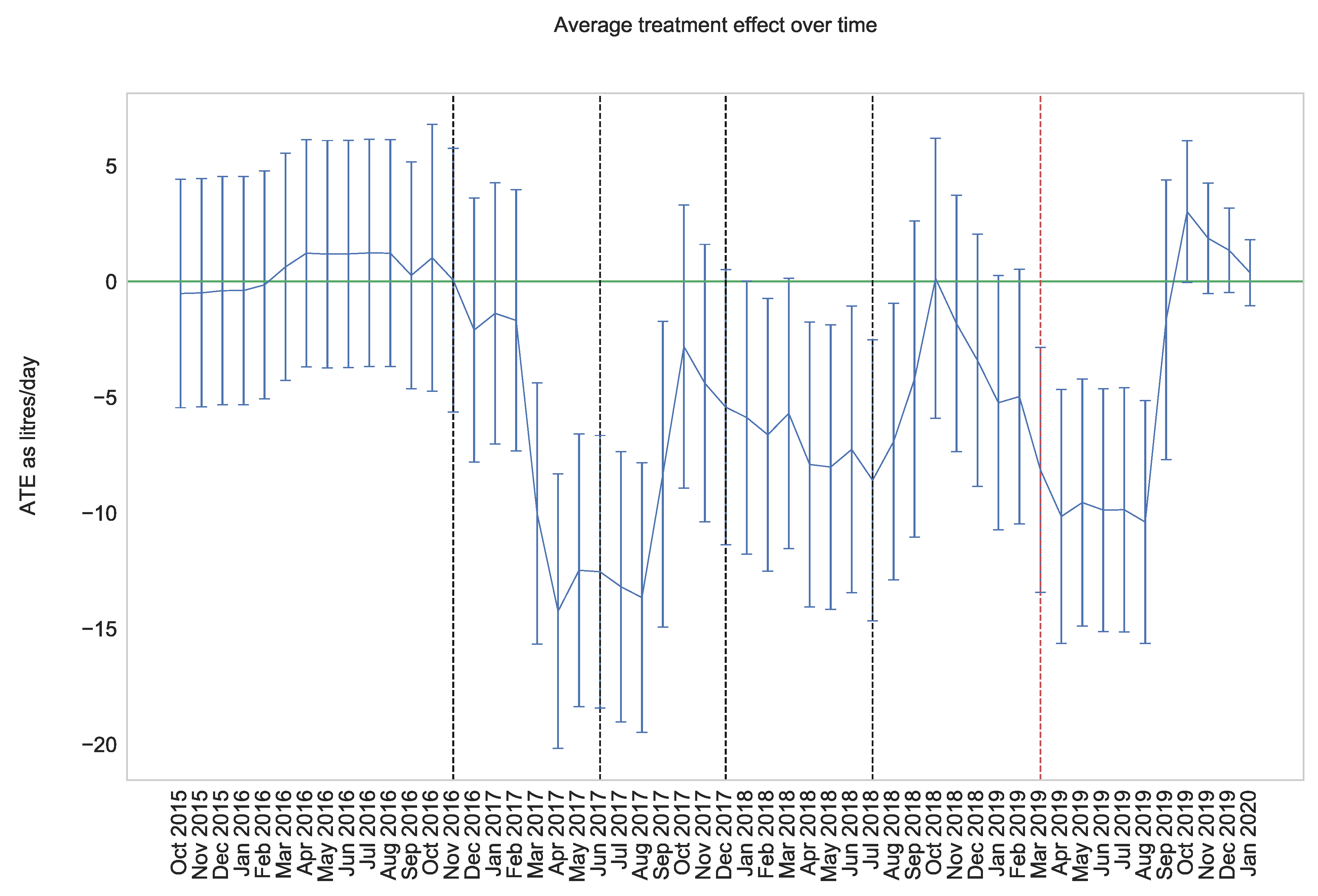
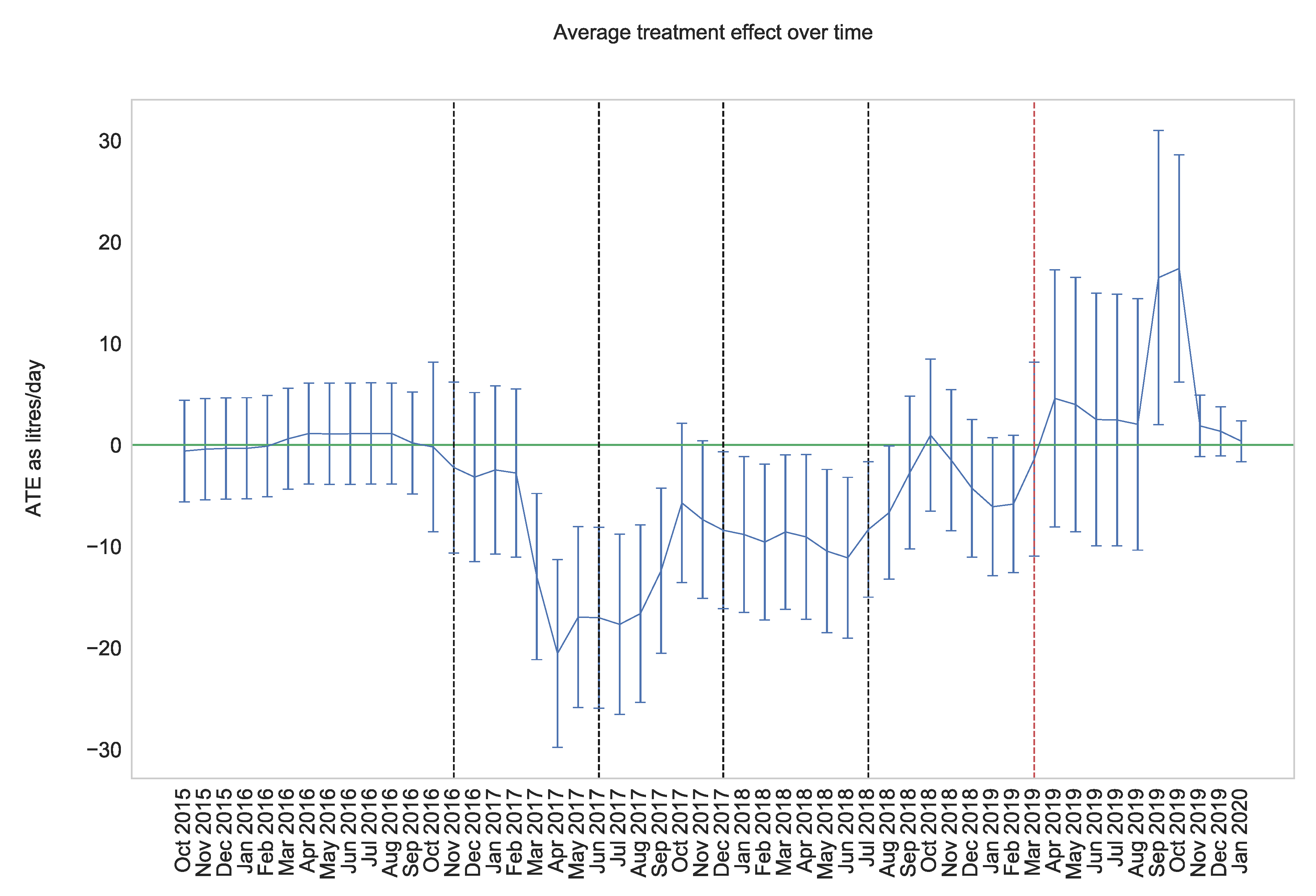
Figure 2 of an event study graph shows the average treatment effect across each month of the entire programme based on the model above. This was calculated by running the regression with an interaction term between group assignment and month. Figure 2 demonstrates the fluctuation in the treatment effect across the programme period, with the greatest reductions occurring in the first summer months. Furthermore, the average treatment effect appears to not be as strong as in the first year, with greater increases in consumption being observed until the end of the programme.
3.2. Quantile Treatment Effects
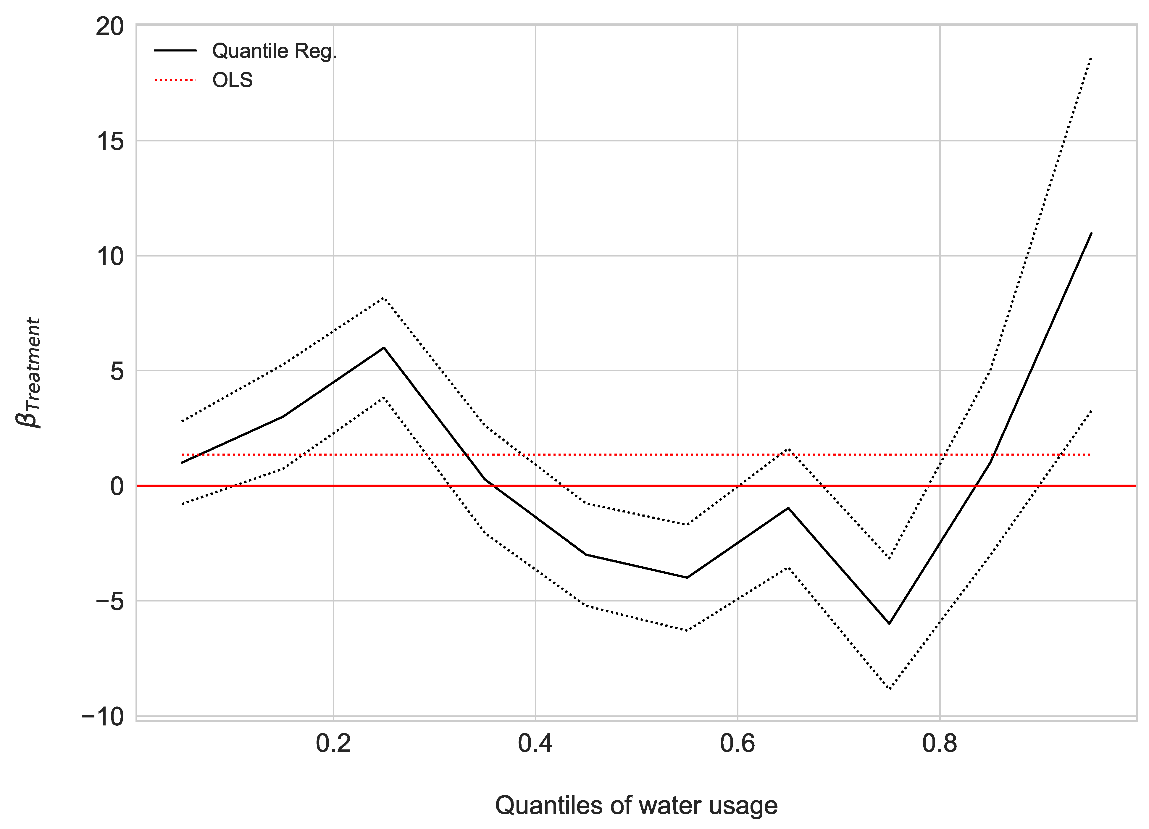
Quantile treatment effects for the first 29 months of the programme can be seen in Figure 3. This was estimated as an unconditional quantile treatment effect with only treatment assignment as the independent variable, and household water consumption in litres per day as the dependent variable. The standard errors were clustered on the household level.
Households in the bottom 20% seem to be increasing their consumption, suggesting a potential boomerang effect whereby being labelled “Efficient Neighbours” may have licensed them to increase their consumption. The greatest reduction in consumption appears to occur across the middle distribution. There also appears to be some households that are notably increasing their consumption as evidenced by the mass moving out to the upper tail. This could be households that have been labelled as high consumers giving up on being efficient. Without a rank invariance assumption, however, these statements are only suggestive.
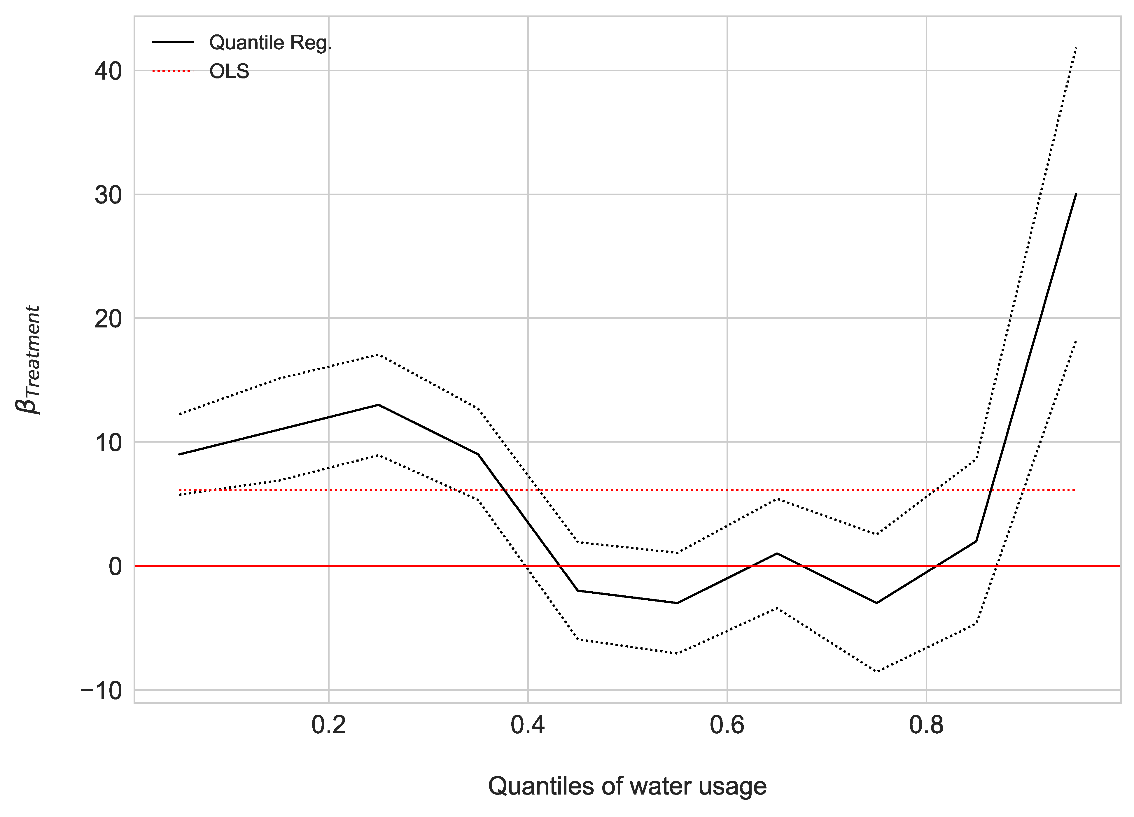
Figure 4 shows quantile treatment effects for the 10 months after the final treatment was delivered. As a purely exploratory interpretation, it appears as though those in the bottom quantiles are increasing their consumption at a slower rate, while those in the top quantiles are increasing their consumption at a faster rate. Overall, the similarity in shape between Figure 3 and Figure 4 suggests that the decay of treatment effect occurs relatively similarly across most of the distribution.
3.3. Conditional Average Treatment Effects
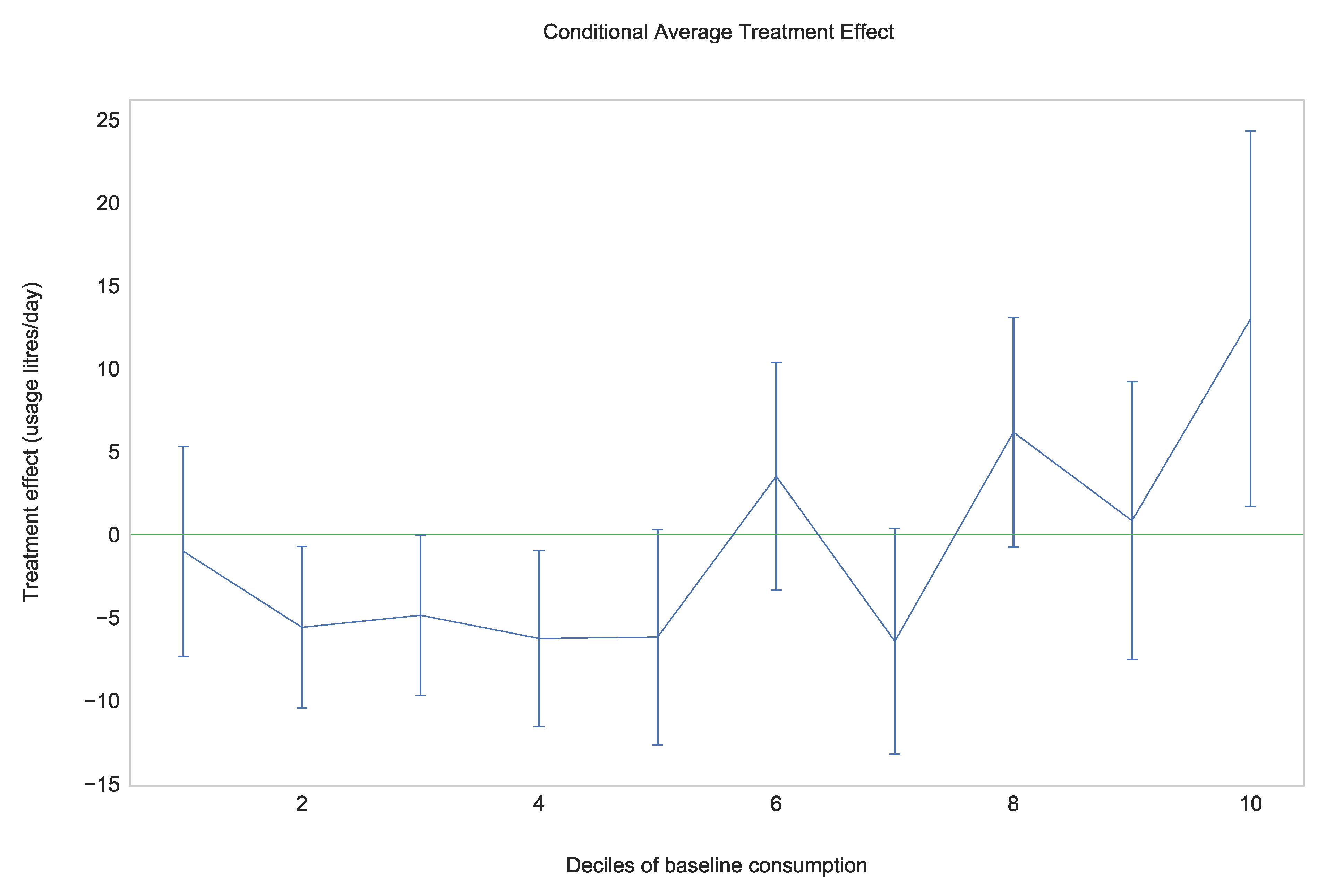
Heterogeneity of treatment effects is also examined by interacting the treatment effect with decile bins of baseline water consumption. Therefore, when observing the treatment effect for the upper deciles of baseline consumption the focus is on households in the sample that populate the high end of the consumption distribution during the baseline period. Figure 5 below suggests that it is mostly households in the lower deciles that reduce their water consumption. These results are more interpretable than the quantile treatment effects because we can observe how the treatment effect differed based on the different household groups, based on their baseline consumption.
3.4. Survey Analysis
Following one year of the programme, South East Water recruited a survey company to interview a random sample of 200 customers in the treatment group. These surveys are conducted regularly as part of SEW’s process of monitoring customer satisfaction. For this round of the survey, additional questions were included to enquire about the programme specifically. Out of the 200 customers surveyed, 87% recalled receiving the home water report, and around half of those read the report thoroughly. In total, 60% of those who recalled receiving the report said that they were satisfied with the programme. The social norms aspect of the report was cited to be the most popular aspect.
4. Discussion
The current paper looks at the effects of a social norms based eco-feedback intervention on household water use in the UK. Results showed that, in line with the hypothesis, the social norms based eco-feedback interventions effectively reduce household water consumption by 1.8%. This effect appears to be highest during the summer months, which is likely because there is more scope for water conservation by reducing non-essential water use such as watering gardens during these months. The effect also appears to be stronger at the beginning of the programme than at the end. The 1.8% average treatment effect is smaller than those observed in the US and Colombia studies. This may be because water consumption in the UK is generally lower than that found in the US and Colombia, so there is less scope for improvement. This is similar to the findings in energy-focused interventions, that effect sizes in Europe are smaller than those in the US, due to the lower energy consumption in Europe [24,25]. The average water consumption of an individual living in the US is around 400 L per day, whereas in the UK it is 141 L per day.
Unlike that seen by Allcott and Rogers [35], these results do not show any ‘action and backsliding’ of treatment effects following the delivery of each home report. This could be due to the lower frequency in which the meters are read, which was six-monthly instead of daily. The lower frequency reads make it much harder to notice immediate and subtle changes in behaviour. Similarly, unlike that seen in Allcott and Rogers [35], no habit formation was observed following the end of the programme. Instead of ‘action and backsliding’ occurring on a monthly or quarterly level that gradually takes stock, the low frequency of six-monthly treatments may allow too much backsliding to occur so that habits are unable to be formed. This interpretation of a decay in treatment effect over the course of the programme should be made with caution because of the attrition in the number of households receiving the treatment over time and the general attrition of available data for households. The low frequency at which the treatment was delivered might also explain the smaller average treatment effect found in this experiment compared to other similar studies where treatment was delivered monthly [26,28,30,31,33]. In Allcott [19], treatment delivered at quarterly intervals had an effect size 0.5% smaller than when treatment was delivered at monthly intervals.
Assuming rank invariance, the analysis of quantile treatment effects suggests the presence of a boomerang effect. Households in the bottom 20% seem to increase their consumption quite sharply. These may be the households that have received feedback labelling them as the top 20% most ‘Efficient Neighbours’, which could licence them to increase their consumption. If this is the case, this would suggest that the intervention’s injunctive norm component failed to counter the boomerang effect, counter to that found in other studies [15,31]. Furthermore, those in the top 20% also increased their consumption sharply. It may be that certain households experienced psychological reactance to the social norms messaging, and chose to increase their consumption in response to feeling pushed to reduce their consumption by their utility [36]. These results differ from that found by Ferraro and Miranda [23], and Allcott [32], as neither interventions increased consumption across the entire distribution.
The heterogeneity analysis based on CATE of baseline consumption suggests that households with lower consumption at baseline were decreasing their consumption the most. This would suggest that counter to the findings of the quantile treatment effects based on an assumption of rank invariance, a boomerang effect may not be present. The intervention is mostly only effective on households that were already relatively low consumers. This finding is in line with previous studies that also utilised injunctive norms to encourage already efficient consumers to keep reducing their consumption. Unlike those previous studies though, the current finding does not find any reduction in consumption for households that were high consumers at baseline. One explanation for these differences could be that low consuming households that already cared about conservation were affected by the motivational effects of the injunctive norm messaging, whereas high consumers were not fazed by the message of the descriptive norm, or were experiencing psychological reactance. Alternatively, high consumers may have simply felt that the goal of reducing their consumption was too great and unachievable, leading to disengagement.
Overall, as these results do differ from that of previous norms based eco-feedback interventions, it cannot be assumed that these interventions will bear the same results in all contexts. This is especially the case when studying the heterogeneity of the treatment effect. Different sub-populations will respond differently to these interventions, and these differences need to be better understood to fully maximise the impact of such treatment across all populations. At the very least, sub-populations that may negatively respond to these interventions may need to be identified and excluded from receiving the intervention.
5. Conclusions
This study demonstrates that while some aspects of the results may differ, social norms based eco-feedback is an effective intervention for reducing water household water consumption in the UK, even with infrequent 6-monthly communications. These effects may not, however, persist once the intervention is stopped. This study has several limitations, including the lack of additional measures of the households to help build a more precise model estimation and better interpret the findings and identify potential mechanisms. For example, not knowing when households are billed means that I cannot control for the effect of receiving a water utility bill on consumption. Not having more detailed information about the type of property or the occupants’ demographics means that I am not able to control for factors that make a difference to their consumption patterns or attribute any heterogeneity in treatment effects to these group differences. A pre-intervention survey to gather this data was not conducted because it was not seen as commercially viable. The additional insights gained from such data would not be beneficial because this type of data would typically not be readily available. Therefore, when the intervention is scaled up, these additional insights would not be actionable. For example, even if it is found that pro-environmental people do not respond to these interventions, and so there is no need to target them, this characteristic would not be observable amongst households prior to an intervention when scaling the programme up.
An additional limitation, as previously mentioned, is that the low frequency of meter reads meant that changes in behaviour were more difficult to detect, and that the frequency of the treatment was also limited. This may be an argument for the promotion of smart meters that provide higher frequency reads. Nonetheless, the current study provided additional evidence for policymakers to recognise the value of utilising social norms based eco-feedback to reduce household water consumption. The current study also helps to further generalise the potential effects of this type of intervention by demonstrating its effectiveness in a novel context.
Future studies may benefit from identifying ways to increase the impact and effectiveness of these interventions. This may be done through differences in how the intervention is delivered (e.g., greater frequency to increase its long term effects) or by leveraging the heterogeneity of the treatment effect to develop a more targeted approach to delivering the intervention.
Funding
This research received no external funding.
Institutional Review Board Statement
The study was conducted according to the guidelines of the Declaration of Helsinki, and approved by the Institutional Review Board (or Ethics Committee) of London School of Economics (Ref: 18284 on 7 December 2020).
Informed Consent Statement
Patient consent was waived due to the treatment being provided as part of normal business services by South East Water for its customers.
Data Availability Statement
Restrictions apply to the availability of these data due to the EU General Data Protection Regulation. Data was obtained from South East Water and Advizzo, and are available from the author with the permission of South East Water.
Conflicts of Interest
The author was employed by Advizzo, the company that delivered the intervention on behalf of South East Water. The design of the experiment was a joint process between Advizzo and South East Water. South East Water conducted data collection of household water use through its meter vendors as part of its usual business operation. The author worked alone in the analysis and interpretation of the data and the writing of this manuscript. While South East Water have sign-off privilege of this manuscript, to determine whether they would want to anonymise themselves or not, no one from Advizzo has seen a copy of this prior to submission for publication.
Appendix A
Figure A1.
Event study graph of changes in the effect size of the intervention across all months of the programme using data without the removal of outliers below and above the 1st and 99th percentile.
Figure A1.
Event study graph of changes in the effect size of the intervention across all months of the programme using data without the removal of outliers below and above the 1st and 99th percentile.

References
- The 11 cities most likely to run out of drinking water—Like Cape Town. BBC News, 11 February 2018.
- Wada, Y.; Flörke, M.; Hanasaki, N.; Eisner, S.; Fischer, G.; Tramberend, S.; Satoh, Y.; van Vliet, M.T.H.; Yillia, P.; Ringler, C.; et al. Modeling global water use for the 21st century: The Water Futures and Solutions (WFaS) initiative and its approaches. Geosci. Model Dev. 2016, 9, 175–222. [Google Scholar] [CrossRef] [Green Version]
- Lawson, R.; Marshallsay, D.; DiFiore, D.; Rogerson, S.; Meeus, S.; Sanders, J.; Horton, B. The Long Term Potential for Deep Reductions in Household Water Demand. Available online: https://www.ofwat.gov.uk/wp-content/uploads/2018/05/The-long-term-potential-for-deep-reductions-in-household-water-demand-report-by-Artesia-Consulting.pdf (accessed on 12 December 2020).
- Boretti, A.; Rosa, L. Reassessing the projections of the World Water Development Report. NPJ Clean Water 2019, 2, 1–6. [Google Scholar] [CrossRef]
- Hussien, W.A.; Memon, F.A.; Savic, D.A. Assessing and Modelling the Influence of Household Characteristics on Per Capita Water Consumption. Water Resour. Manag. 2016, 30, 2931–2955. [Google Scholar] [CrossRef] [Green Version]
- Reynaud, A.; Romano, G. Advances in the Economic Analysis of Residential Water Use: An Introduction. Water 2018, 10, 1162. [Google Scholar] [CrossRef] [Green Version]
- Lehner, M.; Mont, O.; Heiskanen, E. Nudging—A promising tool for sustainable consumption behaviour? J. Clean. Prod. 2016, 134, 166–177. [Google Scholar] [CrossRef]
- Carver, C.S.; Scheier, M.F. Cybernetic Control Processes and the Self-Regulation of Behavior. Oxf. Handb. Hum. Motiv. 2012, 1–30. [Google Scholar] [CrossRef]
- Kluger, A.N.; DeNisi, A. The effects of feedback interventions on performance: A historical review, a meta-analysis, and a preliminary feedback intervention theory. Psychol. Bull. 1996, 119, 254–284. [Google Scholar] [CrossRef]
- Buchanan, K.; Russo, R. Going the extra green mile: When others’ actions fall short of their responsibility. J. Environ. Psychol. 2015, 42, 82–93. [Google Scholar] [CrossRef] [Green Version]
- Karlin, B.; Zinger, J.F.; Ford, R. The effects of feedback on energy conservation: A meta-analysis. Psychol. Bull. 2015, 141, 1205–1227. [Google Scholar] [CrossRef]
- Fischer, C. Feedback on household electricity consumption: A tool for saving energy? Energy Effic. 2008, 1, 79–104. [Google Scholar] [CrossRef]
- Abrahamse, W.; Steg, L.; Vlek, C.; Rothengatter, T. A review of intervention studies aimed at household energy conservation. J. Environ. Psychol. 2005, 25, 273–291. [Google Scholar] [CrossRef]
- Cialdini, R.B.; Trost, M.R. Social influence: Social norms, conformity and compliance. In The Handbook of Social Psychology, 4th ed.; McGraw-Hill: New York, NY, USA, 1998; Volumes 1–2, pp. 151–192. ISBN 978-0-19-521376-8. [Google Scholar]
- Schultz, P.W.; Nolan, J.M.; Cialdini, R.B.; Goldstein, N.J.; Griskevicius, V. The Constructive, Destructive, and Reconstructive Power of Social Norms. Psychol. Sci. 2007, 18, 429. [Google Scholar] [CrossRef] [PubMed] [Green Version]
- Perkins, H.W. Social Norms and the Prevention of Alcohol Misuse in Collegiate Contexts. J. Stud. Alcohol/Suppl. 2002, 14, 164–172. [Google Scholar] [CrossRef]
- Mahler, H.I.M.; Kulik, J.A.; Butler, H.A.; Gerrard, M.; Gibbons, F.X. Social norms information enhances the efficacy of an appearance-based sun protection intervention. Soc. Sci. Med. 2008, 67, 321–329. [Google Scholar] [CrossRef] [Green Version]
- Bicchieri, C.; Dimant, E. Nudging with care: The risks and benefits of social information. Public Choice 2019. [Google Scholar] [CrossRef] [Green Version]
- Czajkowski, M.; Zagórska, K.; Hanley, N. Social norm nudging and preferences for household recycling. Resour. Energy Econ. 2019, 58, 101110. [Google Scholar] [CrossRef]
- Kandul, S.; Lang, G.; Lanz, B. Social comparison and energy conservation in a collective action context: A field experiment. Econ. Lett. 2020, 188, 108947. [Google Scholar] [CrossRef]
- Sherif, M. The Psychology of Social Norms; Harper: Oxford, UK, 1936. [Google Scholar]
- Nolan, J.M.; Schultz, P.W.; Cialdini, R.B.; Goldstein, N.J.; Griskevicius, V. Normative Social Influence is Underdetected. Pers. Soc. Psychol. Bull. 2008, 34, 913–923. [Google Scholar] [CrossRef]
- Allcott, H. Social norms and energy conservation. J. Public Econ. 2011, 95, 1082–1095. [Google Scholar] [CrossRef] [Green Version]
- Andor, M.A.; Gerster, A.; Peters, J.; Schmidt, C.M. Social Norms and Energy Conservation Beyond the US. J. Environ. Econ. Manag. 2020, 103, 102351. [Google Scholar] [CrossRef]
- Bonan, J.; Cattaneo, C.; d’Adda, G.; Tavoni, M. The interaction of descriptive and injunctive social norms in promoting energy conservation. Nat. Energy 2020, 5, 900–909. [Google Scholar] [CrossRef]
- Brent, D.A.; Cook, J.H.; Olsen, S. Social Comparisons, Household Water Use, and Participation in Utility Conservation Programs: Evidence from Three Randomized Trials. J. Assoc. Environ. Resour. Econ. 2015, 2, 597–627. [Google Scholar] [CrossRef]
- Schultz, P.W.; Messina, A.; Tronu, G.; Limas, E.F.; Gupta, R.; Estrada, M. Personalized Normative Feedback and the Moderating Role of Personal Norms: A Field Experiment to Reduce Residential Water Consumption. Environ. Behav. 2016, 48, 686–710. [Google Scholar] [CrossRef] [Green Version]
- Jaime Torres, M.M.; Carlsson, F. Direct and spillover effects of a social information campaign on residential water-savings. J. Environ. Econ. Manag. 2018, 92, 222–243. [Google Scholar] [CrossRef]
- Ferraro, P.; Price, M. Using Non-Pecuniary Strategies to Influence Behavior: Evidence from a Large Scale Field Experiment. Rev. Econ. Stat. 2013, 95, 64–73. [Google Scholar] [CrossRef]
- Bhanot, S.P. Rank and response: A field experiment on peer information and water use behavior. J. Econ. Psychol. 2017, 62, 155–172. [Google Scholar] [CrossRef]
- Bhanot, S.P. Isolating the effect of injunctive norms on conservation behavior: New evidence from a field experiment in California. Organ. Behav. Hum. Decis. Process. 2018, 1–13. [Google Scholar] [CrossRef] [Green Version]
- Ferraro, P.J.; Miranda, J.J. Heterogeneous treatment effects and mechanisms in information-based environmental policies: Evidence from a large-scale field experiment. Resour. Energy Econ. 2013, 35, 356–379. [Google Scholar] [CrossRef]
- Ferraro, P.J.; Miranda, J.J.; Price, M.K. The Persistence of Treatment Effects with Norm-Based Policy Instruments: Evidence from a Randomized Environmental Policy Experiment. Am. Econ. Rev. 2011, 101, 318–322. [Google Scholar] [CrossRef] [Green Version]
- Ayres, I.; Raseman, S.; Shih, A. Evidence from Two Large Field Experiments that Peer Comparison Feedback Can Reduce Residential Energy Usage. J. Law Econ. Organ. 2013, 29, 992–1022. [Google Scholar] [CrossRef]
- Allcott, H.; Rogers, T. The short-run and long-run effects of behavioral interventions: Experimental evidence from energy conservation. Am. Econ. Rev. 2014, 104, 3003–3037. [Google Scholar] [CrossRef] [Green Version]
- Brehm, J.W. Psychological Reactance: Theory and Applications. Adv. Consum. Res. 1989, 16, 72–75. [Google Scholar]
Figure 1.
An example of the home report sent to households in the treatment group.

Figure 2.
Event study graph of changes in the intervention’s average treatment effect in litres per day across all months of the pre and post-intervention period. The coefficients and standard error were generated from interacting treatment assignment with monthly dummy variables while controlling for baseline consumption. Each vertical dashed line indicates when the intervention was administered. Note: the version of this graph in Appendix A uses the dataset that does not remove outliers above and below the 1st and 99th percentiles, and shows a stronger upward trend after month 29.

Figure 3.
Quantile treatment effects for the treatment across the first 29 months of the intervention. The dotted red line represents the average treatment effect, while the black line represents the quantile treatment effect. Dotted lines represent the 95% confidence intervals. Standard errors were clustered on the household level.

Figure 4.
Quantile treatment effects for the treatment across the 10 months after the last home report was sent. The red line represents the average treatment effect, while the black line represents the quantile treatment effect. Dotted lines represent the 95% confidence intervals.
Figure 4.
Quantile treatment effects for the treatment across the 10 months after the last home report was sent. The red line represents the average treatment effect, while the black line represents the quantile treatment effect. Dotted lines represent the 95% confidence intervals.

Figure 5.
Graph showing the average treatment effect (y-axis) conditional on 10 bins of baseline consumption (x-axis) during the first 29 months of the programme. On the x-axis, 1 represents households with low water usage during the baseline period, while 10 represents the highest usage. The coefficients and standard error were extracted from a regression with interaction effects between treatment assignment and decile bins of baseline consumption.


Table 1.
Dates of when the home water reports were generated, and the number of households at each of those dates.
Table 1.
Dates of when the home water reports were generated, and the number of households at each of those dates.
| Date When Treatment Was Generated | Number of Households Included |
|---|---|
| 18 November 2016 | 1949 |
| 16 June 2017 | 1768 |
| 9 December 2017 | 1559 |
| 30 July 2018 | 1277 |
| 19 February 2019 | 1035 |
Publisher’s Note: MDPI stays neutral with regard to jurisdictional claims in published maps and institutional affiliations. |
© 2021 by the author. Licensee MDPI, Basel, Switzerland. This article is an open access article distributed under the terms and conditions of the Creative Commons Attribution (CC BY) license (http://creativecommons.org/licenses/by/4.0/).
Share and Cite
MDPI and ACS Style
Ramli, U. Social Norms Based Eco-Feedback for Household Water Consumption. Sustainability 2021, 13, 2796. https://doi.org/10.3390/su13052796
AMA Style
Ramli U. Social Norms Based Eco-Feedback for Household Water Consumption. Sustainability. 2021; 13(5):2796. https://doi.org/10.3390/su13052796
Chicago/Turabian StyleRamli, Ukasha. 2021. "Social Norms Based Eco-Feedback for Household Water Consumption" Sustainability 13, no. 5: 2796. https://doi.org/10.3390/su13052796
Note that from the first issue of 2016, this journal uses article numbers instead of page numbers. See further details here.