Fiscal and Budgetary Policy Efforts towards Climate Change Mitigation in Romania

Abstract

To mitigate the negative effects of climate change on the environment, the Member States of the European Union implement fiscal measures and commit budgetary expenditures to ensure sustainable economic development. Romania, in line with the Union’s objectives, resorted to the application of a system of environmental taxes and provided in the budgetary policy government expenditures for environmental protection. The aim of the research is to highlight the effects of these measures on the environment by analysing the short-run and long-run causal relationships between greenhouse gas emissions, green taxes and government expenditures on environmental protection. Autoregressive Distributed Lag (ARDL) method and Granger causality tests were used to demonstrate the existence of these relationships and the intensity with which they manifest. Following the analysis, we identified a significant long-run influence of government spending on environmental protection on greenhouse gas emissions but also numerous short-run and long-run causal relationships between greenhouse gas emissions and green taxes, applied in Romania. The results of the research consider the impact of public expenses for environment protection, a variable not yet applied for Romania, on greenhouse gas emissions’ decrease, in correlation with environmental taxes per source of origin.

1. Introduction

Climate change is a reality that cannot be denied. This challenge should be seen from various perspectives: that of mitigation when governments try to reduce the dimension of climate change using different strategies and policies, adaptation when the harm is done but governments implement measures meant to reduce the impact of greenhouse gas (GHG) emissions on the environment and human life and also risk management specific to disasters when the world should be prepared for the worst scenario.

According to World Meteorological Organization [1], in 2020, there was registered a record on the long-lasting ozone hole over the Atlantic (from mid-August until the end of December). A report of the same organization [2] mentions a few records in 2018 when GHG emissions reached important levels, in 2019 considered the second warmest year after 2016 when the average temperature registered globally was above the preindustrial levels with 1.1 °C. The rise in GHG emissions is the most important cause for climate change and the most evident indicator for this is the temperature.

Thus, leaders of the world established important goals related to the target of net-zero emissions until 2050. However, the World Meteorological Organization [2] considers the risk of not achieving this goal is considerable taking into account the new data according to which the levels of GHG emissions increase with each year. The UN Climate Change Conference that should have taken place in November 2020 was unfortunately postponed for 2021 due to the pandemic situation [3]. Serious questions regarding the policies and strategies that should be implemented at the level of each state are a priority for this conference.

The European Parliament [4] analyses the problem of climate change from a budgetary perspective. Fiscal measures implemented by the European Union member states and targeted budgetary decisions can have a direct impact on GHG emissions. Starting from 2011, 20% of the EU budget is used for climate change mitigation. This level was changed in December 2020 to 30% for the next seven years [5]. In their latest report, the European Investment Bank [6] announced their intention to direct 50% of their budgets to finance climate action meant to reduce GHG emissions and protect the environment.

CAN Europe [7] published the ranking of countries in European Union in terms of their fight against climate change. Thus, countries like Sweden (good), Portugal, France, Netherlands, and Luxembourg (moderate) are having better policies dedicated to climate action, compared to the countries at the bottom of the ranking such as Cyprus, Malta, Bulgaria, Estonia, Ireland, and Poland (very poor). Countries between these extremes are characterized as having a poor effort in mitigating climate change.

In order to protect the environment and reduce GHG emissions, governments adopt environmental policies that are strongly intercorrelated with fiscal and budgetary policies. Governments increase their revenues by applying environmental taxation and use these revenues to adopt measures that mitigate climate change or prevent future deterioration of the environment.

One of the solutions for climate change mitigation is represented by Environmental Tax Reform (ETR), using both taxation on energy, transportation and pollution and also expenses for environmental protection, green investments, meant to adjust the infrastructure to climate change and reduce other taxes such as that on labour [8,9].

Even though national environmental taxation in some of the member countries in the European Union is a reality, there are debates related to imposing EU-wide taxes on fuels, but this change will require consensus from all countries, a fact unlikely to happen in the nearest future [10,11]. For more efficient results of these policies, there is a need for educating people on these issues. Thus, the European Union created a pilot program, TAXEDU, which is in fact a digital platform meant to educate people on the importance of taxes for society and environment [11].

One of the reasons green taxation is efficient is because these taxes influence the price of some products and services and in the end the consumers’ decision and buying preferences. The objective is to discourage the use of products and services that are not environmentally friendly and encourage greener choices. There can appear important shifts on the market related to changes in demand and supply.

Andersson et al. [12] appreciate that fiscal measures targeting climate change mitigation are having a “net impact on public finances” that is not very clear, because besides the revenues from the taxes, there are numerous expenses related to changes in the infrastructure and other public expenditures needed for environmental protection.

If the consumption of some products that are taxed decreases, the revenues will also decrease, so there is a need to offer fiscal incentives for encouraging the consumption of more efficient products from an environmental perspective. Furthermore, these products can contribute to an increase of revenues on the long term. Usually, people make the transition to greener products not so easily because the other products or services offer something more important for them on a short term (a cheaper price or another benefit like a shorter duration of transportation). This is the reason for which governments subsidize the transition to the products and offer financial support for people transitioning to more efficient products, with a lower consumption of energy.

The purpose of the present research is to analyse the effort exerted by public authorities in Romania, as a member state of the European Union, in mitigating climate change by using fiscal instruments (environmental taxes) and budgetary ones (government expenditures for environmental protection). In this sense, the relationship of causality between GHG emissions, revenues from taxes on energy, transportation and pollution/ resources and government expenditures for environment protection. This relationship is important because it offers a better understanding of the way GHG emissions can be reduced in both the short and the long-term using fiscal and budgetary policies.

The paper is structured taking into account the following sections: the literature review part, focusing on the most important studies based on the relationship between fiscal policies and GHG emissions; the methodology part, where the equation at the basis of the research and the two hypotheses regarding the relationship between environment taxation, public expenses for the environment protection and the reduction of GHG emissions are presented; the results and discussion section where the strong connection between fiscal policies with an environmental component and climate change mitigation is underlined.

2. Literature Review

OECD [13] highlights that there is an important risk of not reaching the goals established within the Paris Agreement taking into account recent numbers on GHG emissions worldwide. Therefore, not only environmental taxes are useful but also the creation of international emissions trading systems (ETS). In 2005, the European Union launched the first market of this type [14].

Fiscal and budgetary policies and all the other mechanisms on the market can contribute to the goal of net-zero emissions for 2050. This does not mean that there will not be GHG emissions anymore, but they will be reduced to a minimum and also there will be investments in the development of new technologies that will reduce or even remove the emissions in the atmosphere, in order to maintain the balance and keep the temperature to normal limits.

The double dividend theory refers to the two benefits brought by environmental taxation: on one hand, there is the environmental protection and on the other hand, the revenues collected by the governments that can be used to stimulate the economy cutting other taxes and thus not affecting the competitiveness of industries in developing countries.

The literature review covers contradicting opinions regarding this subject. Nerudová and Dobranschi consider that the second dividend is not seen in all contexts and sometimes a reduction in income taxes can have a negative impact on the environment [15], the authors suggest that “capital or payroll taxes cuts” can be more efficient in ensuring double dividend. The importance of taxation is also highlighted by Ghazouani et al. [16] who appreciate that climate changes are generated by developed countries where there is a “growth in income, population, energy intensity”.

Thus, economic development that is connected to the notion of social responsibility and fiscal policies meant to contribute to a reduction of GHG emissions should be seen as such. Here comes the importance of education of all citizens in order to accept taxation on pollution, energy and transportation that might affect the environment on the long term. Another opinion on the double dividend theory emphasizes that policymakers should take risks, otherwise it might be too late for the environment [17].

The fiscal and budgetary policies have an important impact on energy consumption and on the buying behaviour of a country’s population and also on the technologies used in production by companies [18]. Thus, there are numerous variables that should be considered by governments when deciding the most appropriate structure of taxes to mitigate climate change, because these can impact the economic performance of companies [19] or the differences in the level of development of the various regions of a country [20]. Zaharia et al. [21] consider that policymakers have to use both “punitive measures” by taxation and also promote “sustainable practices”. Włodarczyk et al. [22] highlight the importance of finance for the survival of a business, so the public policies should take into account the impact on the small and medium enterprises. Similarly, Ionescu et al. [23] show that environmental factors, besides others, influence the company in terms of performance, an additional reason for the government to take into account companies when establishing environmental policies and take fiscal measures to mitigate climate changes. All the innovations, needed for the companies to become more environment friendly, have an important impact on the financial development of these businesses [24].

Vallés-Giménez and Zárate-Marco [25] analyse the impact of environmental taxation on different regions of Spain and concludes that more “aggressive policies” are needed in order to have a significant reduction in GHG emissions. The authors also consider that environmental taxation should not be applied only to industry, because this can suffer dramatically but to other sectors too. Thus, they appreciate that a Europe-wide taxation on GHG emissions might be more efficient than the present EU-ETS. Solilová and Nerudová [26] also conclude that EU-ETS is not so efficient, not generating enough “investments in low-carbon technologies”.

Another study [27] emphasizes the need to take into account not only taxation for mitigating climate changes but also the shifts in demand. Consumers should be incentivized to buy products that are more efficient and friendly to the environment. The authors appreciate that the European Directive on energy taxation does not take into consideration these “financial incentives” and should be amended accordingly.

Andreoni [28] makes an analysis on the structure of the revenues from environmental taxation among 25 of the EU countries between 2004 and 2016 and also on the factors that influence these revenues for a country. Thus, developed countries such as Belgium, Denmark, Germany, France, Netherlands, Austria, Finland and United Kingdom are characterised by an increase in revenues from environmental taxes generated mostly by their economic growth. At the opposite pole, there are countries like Romania, Bulgaria, Slovakia, Estonia, Latvia, Lithuania, Poland, Czech Republic, where the leading factor for the increase of revenues from green taxation is represented mostly by structural changes specific to developing countries and not so much by economic growth.

Shahbaz et al. [29] tested Environmental Kuznets Curve for Romania using variables such as energy consumption, economic growth and carbon dioxide (CO₂) emissions but without taking into consideration the fiscal policy of the country which has an important impact on these variables. Other authors [30] conducted a broader analysis of the implications of energy taxation on both the economy and the environment, investing the causality between energy taxation, gross domestic product, CO₂ emissions, renewable and nonrenewable energy.

Chițiga [31] also makes an analysis of the energy taxes in Romania and the revenues generated by them in comparison with the other EU member states with a focus on former communist countries. Barbu [32] analyses the structure of the sources contributing to the Environmental Fund in Romania and concludes that “there is… uncertainty about the long-term structure of environmental taxes in Romania”. Radulescu et al. [33] conducted a research on the double dividend theory of environmental taxes in Romania, highlighting that there are still many differences among EU countries regarding environmental policies. The authors appreciate that environmental protection benefit is more evident in Romania than the economic growth benefit, in comparison to the other countries in the EU. As other papers mentioned [21,27], besides taxation, there is a need for offering financial incentives for people and companies to stimulate the economy and direct it to a greener one in the future, thus raising the chances of reaching the net-zero emissions goal established for the year 2050.

3. Materials and Methods

3.1. Research Hypotheses

In order to reach the proposed aim, two research hypotheses were planned based on the relationship between environment, green taxes and public expenses for environment protection:

Hypothesis 1 (H1).

A growth in revenues from environment taxes determines a decrease in greenhouse gas emissions in Romania;

Hypothesis 2 (H2).

The governmental expenses for environment protection will have a long-term contribution to climate change mitigation.

3.2. Data and Indicators

The approach of the current research is based on the theories regarding the role of environment taxes (the theory of the first dividend and the theory of the Kuznets curve), together with the implication of the national public authorities on the step towards a sustainable economic development.

The article underlines the effects resulting from implementing environment taxes and governmental expenses for environment protection on greenhouse gas emissions (GHG). Climate mitigation aims to decrease emissions of climate-harming greenhouse gases that originate from human activity, through measures such as promoting low-carbon technologies or enhancing GHG sinks by encouraging sustainable forest management and land use policies. Annual change in GHG emissions is a key indicator to track the success of climate mitigation measures. The representative variables within the current research model, for reaching the proposed goal, are explained in

Table 1. Data used in the research model.

Acronim	Variable	Measurement Unit
GHG	Greenhouse gas emissions	tonnes per capita
RET	Total Revenues from Energy taxes	% of GDP
RTT	Total Revenues from taxes on Transport	% of GDP
RTPR	Total Revenues from taxes on Pollution or Resources	% of GDP
GGEXP	Total general government expenditure for environmental protection	million euro

Source: Authors’ own analysis.

. The analysis uses a time series of 23 years, from 1995 to 2018, the data being taken from the official website of the European Commission, Eurostat.

The effects resulted from applying environment taxes and governmental expenses for environment protection on greenhouse gas emissions in Romania are underlined by the causality relationships among them.

3.3. Methodology

In order to verify the two hypotheses, an equation that fragments the environment taxes on sources of origin and also includes the general government expenses for environment protection, a variable that has not previously been analysed in Romania, was used:

GHG_t = α₁ + α₂RET_t+ α₃RTT_t + α₄RTPR_t+ α₅GGEXP_t + ε_t

(1)

where:

• GHG represents the greenhouse gas emissions;
• RET is the total revenues from energy taxes as % of GDP;
• RTT is the total revenues from taxes on transport;
• RTPR is the total revenues from taxes on pollution or resources;
• GGEXP represents the total general government expenditure for environmental protection;
• ε_t is the residual term;
• α_1,…,5 represent the coefficients of the equation
• t is the time.

To identify the causality relationships between greenhouse gas emissions, revenues from taxes on energy, revenues from taxes on transport, revenues from taxes on pollution or resources and governmental expenses for environment protection, the following steps are necessary to be followed to obtain valid results.

Thus, the first step consists in testing the stationarity of the data series used in this equation. Two tests of unit root are used: Augmented Dickey–Fuller Phillips and Perron test. According to Dickey and Fuller (1979) [34], the statistics do not have a conventional Student’s t-distribution, they provide asymptotic results and emphasize critical values for different tests and samples, under the null hypothesis of a unit root. The Augmented Dickey–Fuller (ADF) test provides parametric correction for higher-order correlation, beginning from the assumption that the Y series has the same evolution as an AR(i) process and then adding i-lagged difference terms of the dependent variable Y to the regression:

$$\Delta Y_t={\beta }_1+{\beta }_2\mathrm{t}+\delta Y_{t-1}+{\alpha }_i{\displaystyle \sum }_{\mathrm{i}=1}^{\mathrm{m}}\Delta Y_{t-i}+{\epsilon }_t$$

(2)

Two practical issues will be faced by an ADF test. First, the decision whether to include exogenous variables in the regression has to be taken. There are the following options that can be taken: to include a constant, a constant and a linear time trend or no constant and no linear time trend, in the regression. The test can be analysed with a constant and a linear trend, because the other two cases are considered exceptional cases. The power of the test to reject the null of a unit root can be diminished by including irrelevant regressors in the regression. A specification that is a plausible description of the data under both null and alternative hypotheses (Hamilton, 1994, p. 501) [35] will be chosen. Secondly, the lagged difference terms (“lag length”) from the regression are identified. Several lags sufficient to remove serial correlations in the residuals are also included.

Phillips and Perron (1988) [36] focus on a nonparametric method to control serial correlation when testing for a unit root in the model. The PP method helps estimate the nonaugmented DF test equation and modifies the t-ratio of the β coefficient in such a way that the serial correlation will not influence the asymptotic distribution of the statistics test. The PP test equation is:

$$Z\left(\tau \right)=\tau \left(\frac{{\widehat{\sigma }}^2}{{\widehat{\sigma }}_{sl}^2}\right)-\left(\frac{1}{2}\right)\left({\widehat{\sigma }}_{sl}^2-{\widehat{\sigma }}^2\right)T\sqrt{{\widehat{\sigma }}_{sl}^2{\displaystyle \sum }_{\mathrm{t}=2}^{\mathrm{T}}{\left(x_{t-1}-{\overline{x}}_{T-1}\right)}^2}$$

(3)

The second step consists in the selection of the optimal way depending on the number of lags using Autoregressive Distributed Lag (ARDL) method and graphic representation.

The third step supposes testing the cointegration relationship between greenhouse gas emissions, revenues from taxes on energy, revenues from taxes on transport, revenues from taxes on pollution or resources and governmental expenses for environment protection, using ADRL method. This method is useful for the current research, because it does not take into consideration the integration order of the variables and is recommended for the studies with a low amount of data. The ARDL method supposes testing the cointegration relationships beginning from the following equation that will be applied to every variable included in the analysis:

$$\begin{array}{cc}\hfill \Delta {\mathrm{GHG}}_{\mathrm{t}}=& {\beta }_1+{\displaystyle {\displaystyle \sum }_{i=1}^n}{\alpha }_1\Delta {\mathrm{GHG}}_{t-i}+{\displaystyle {\displaystyle \sum }_{i=1}^n}{\alpha }_2\Delta {\mathrm{RET}}_{t-i}+{\displaystyle {\displaystyle \sum }_{i=1}^n}{\alpha }_3\Delta {\mathrm{RTT}}_{t-i}\hfill \\ & +{\displaystyle {\displaystyle \sum }_{i=1}^n}{\alpha }_4\Delta {\mathrm{RTPR}}_{t-i}+{\displaystyle {\displaystyle \sum }_{i=1}^n}{\alpha }_5\Delta {\mathrm{GGEXP}}_{t-i}+{\varnothing }_1{\mathrm{GHG}}_{t-i}+{\varnothing }_2{\mathrm{RET}}_{t-i}\hfill \\ & +{\varnothing }_3{\mathrm{RTT}}_{t-i}+{\varnothing }_4{\mathrm{RTPR}}_{t-i}+{\varnothing }_5{\mathrm{GGEXP}}_{t-i}+{\epsilon }_{1t}\hfill \end{array}$$

(4)

If ${\varnothing }_1={\varnothing }_2={\varnothing }_3={\varnothing }_4={\varnothing }_5=0$ then null hypothesis of the lack of cointegration between variables is accepted and if ${\varnothing }_1\ne {\varnothing }_2\ne {\varnothing }_3\ne {\varnothing }_4\ne {\varnothing }_5\ne 0$ then it means that cointegration relationships between the variables included in the model exist.

There is a cointegration between the variables of the model if the value of F-statistic is higher than the upper critical bound values. If the value of F-statistic is between the minimum and maximum values of the bounds test, then the existence or nonexistence of a cointegration relationship between variables cannot be determined, and if the value of F-statistic is lower than the lower critical bound, there is no cointegration relationship between the variables of the model.

The stability of the selected model was tested using two of the most relevant and employed tests based on recursive residuals: the cumulative sum of recursive residuals (CUSUM) and the cumulative sum of squares of recursive residuals (CUSUMsq).

The fourth step supposes identifying the causality relationships between the variables throughout the development of a dynamic error correction model (ECM) that integrates short-run causality relationships with those on the long-run, without losing information about the latter. It is important to mention that an equation with an error correction term (ECT) can be estimated only for those equations in which the cointegration relationship is confirmed.

The multivariate Granger causality estimation based on ARDL-ECM and lagged conditions were used to determine short-run and long-run causality among the variables of the model. The equations in the model of this study can be expressed as a system of equations:

$$\begin{array}{cc}\hfill \left[\begin{array}{c}\Delta {\mathrm{GHG}}_t\\ \Delta {\mathrm{RET}}_t\\ \Delta {\mathrm{RTT}}_t\\ \Delta {\mathrm{RTPR}}_t\\ \Delta {\mathrm{GGEXP}}_t\end{array}\right]=& \left[\begin{array}{c}{\delta }_1\\ {\delta }_2\\ {\delta }_3\\ {\delta }_4\\ {\delta }_5\end{array}\right]+\left[\begin{array}{c}{\delta }_{11,1}{\delta }_{12,1}{\delta }_{13,1}{\delta }_{14,1}{\delta }_{15,1}\\ {\delta }_{21,1}{\delta }_{22,1}{\delta }_{23,1}{\delta }_{24,1}{\delta }_{25,1}\\ {\delta }_{31,1}{\delta }_{32,1}{\delta }_{33,1}{\delta }_{34,1}{\delta }_{35,1}\\ {\delta }_{41,1}{\delta }_{42,1}{\delta }_{43,1}{\delta }_{44,1}{\delta }_{45,1}\\ {\delta }_{51,1}{\delta }_{52,1}{\delta }_{53,1}{\delta }_{54,1}{\delta }_{55,1}\end{array}\right]\left[\begin{array}{c}\Delta {\mathrm{GHG}}_{t-1}\\ \Delta {\mathrm{RET}}_{t-1}\\ \Delta {\mathrm{RTT}}_{t-1}\\ \Delta {\mathrm{RTPR}}_{t-1}\\ \Delta {\mathrm{GGEXP}}_{t-1}\end{array}\right]+\dots +\left[\begin{array}{c}{\delta }_{11,i}{\delta }_{12,i}{\delta }_{13,i}{\delta }_{14,i}{\delta }_{15,i}\\ {\delta }_{21,i}{\delta }_{22,i}{\delta }_{23,i}{\delta }_{24,i}{\delta }_{25,i}\\ {\delta }_{31,i}{\delta }_{32,i}{\delta }_{33,i}{\delta }_{34,i}{\delta }_{35,i}\\ {\delta }_{41,i}{\delta }_{42,i}{\delta }_{43,i}{\delta }_{44,i}{\delta }_{45,i}\\ {\delta }_{51,i}{\delta }_{52,i}{\delta }_{53,i}{\delta }_{54,i}{\delta }_{55,i}\end{array}\right]\left[\begin{array}{c}\Delta {\mathrm{GHG}}_{t-i}\\ \Delta {\mathrm{RET}}_{t-i}\\ \Delta {\mathrm{RTT}}_{t-i}\\ \Delta {\mathrm{RTPR}}_{t-i}\\ \Delta {\mathrm{GGEXP}}_{t-i}\end{array}\right]\hfill \\ \hfill +& \left[\begin{array}{c}{\phi }_1\\ {\phi }_2\\ {\phi }_3\\ {\phi }_4\\ {\phi }_5\end{array}\right]\times {\mathrm{ECT}}_{t-1}+\left[\begin{array}{c}{\mu }_{1,t}\\ {\mu }_{2,t}\\ {\mu }_{3,t}\\ {\mu }_{4,t}\\ {\mu }_{5,t}\end{array}\right]\hfill \end{array}$$

(5)

where:

• ECT is the lagged error correction term;
• μ_i,t are the serially independent random errors.

The estimated values of the error correction term show the speed of adjustment from short-run to lung-run equilibrium in the models, depending on the sign of the associated coefficient.

4. Results and Discussions

During recent decades, climate change generated major interest at the level of the European institutions that tried to identify the key factors that lead to environment degradation. Thus, the level of greenhouse gas emissions is considered an important factor in this aspect. The values of the greenhouse gas emissions for the years 1995 and 2018, representing the endpoints of the analysed time series, are represented in the Figure 1. The position of Romania among the European Union member states is underlined.

In most of the states (including Romania), the level of greenhouse gas emissions registered lower values in the year 2018 compared to the year 1995, because of the applied environment policies and the cumulated effort of the institutions and population regarding the environment protection. There are also some exceptions to this trend and thus, in five of the 28 member states of the European Union (Estonia, Croatia, Latvia, Lithuania and Portugal), greenhouse gas emissions registered a higher level in 2018 compared to the year 1995.

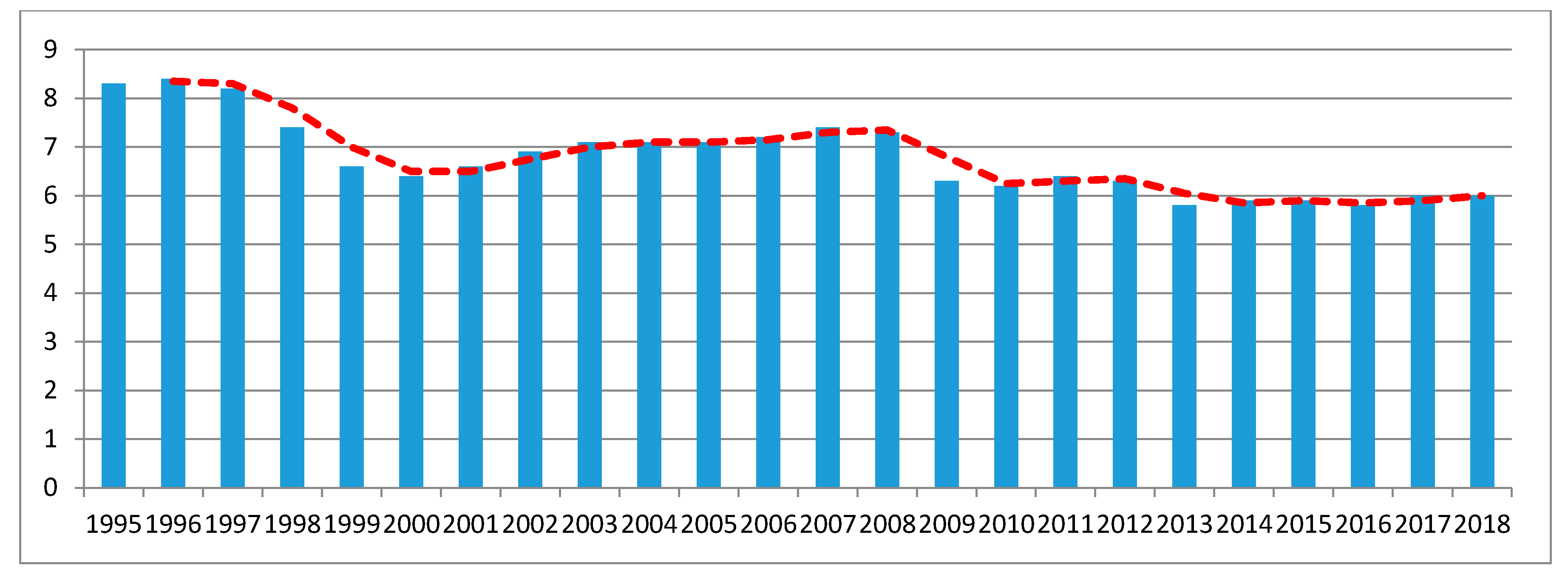
In Romania, this indicator had a positive evolution, decreasing with two points during the analysed period, but the evolution of the greenhouse gas emissions was fluctuating within the analysed time interval, with two sudden decreases for the years 1999–2000 and 2009–2010. However, Romania was on the third place among EU member states with the lowest level of greenhouse gas emissions, after Sweden and Malta, for the year 2018. (Figure 2).

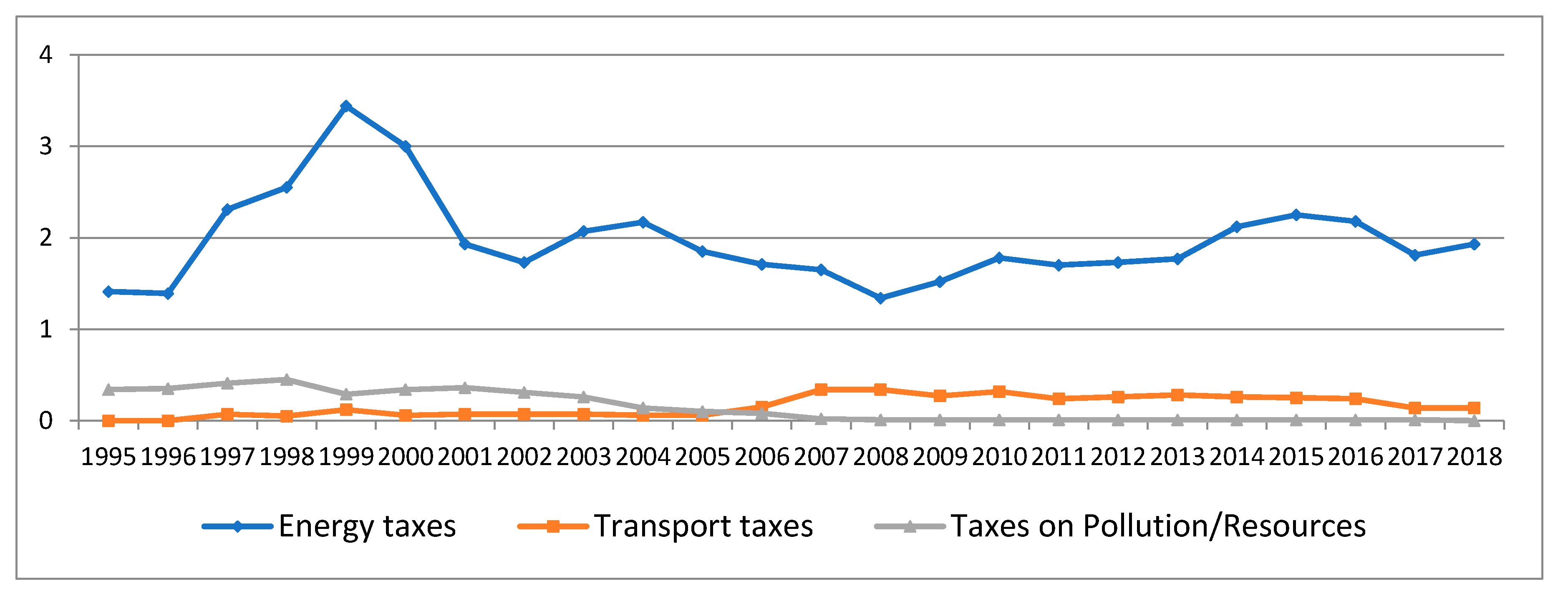
The applied environment policies have a significant contribution to the greenhouse gas emissions’ decrease, with an important place taken by the environment taxes and government expenses for environment protection. The system of environment taxes applied in Romania is complex and efficient, with a double benefit (according to the theory of double dividend), supplying on the one hand, the state budget with financial resources and, at the same time, protecting the environment. The evolution of the revenues gathered from environment taxes, as a percentage of GDP, is presented in Figure 3.

Taxes on energy have a significant percentage in GDP, with a maximal level of 3.44% in 1999 and a minimum level of 1.34% of GDP in 2008, because of the retraction of the economic activity, as a result of the global economic crisis of that year. After the year 2008, the level of revenues from taxes on energy registered a light increase, reaching 1.93% of GDP in 2018.

Taxes on transport and taxes on pollution and resources register a level under 0.5% of GDP. Until the year 2005, the values of the taxes on pollution/ resources were more significant and the taxes on transport registered values close to 0% of GDP. However, beginning with the year 2006, the taxes on pollution/resources had values close to 0% of GDP, while the taxes on transport were close to 0.5% of GDP.

Besides the environment taxes as part of the fiscal policy of Romania, the budgetary policy foresees in the budget a series of governmental expenses for environment protection (Figure 4). The total expenses at the national level include investments, internal current expenses (expenses made by the employees of the organisation), while the external current expenses are excluded (expenses for buying environment protection services from third parties and the taxes paid as environment taxes). Investments for environment protection include all capital expenses linked to environment protection (implying methods, processes, technologies, equipment or parts of those) whose major goal consists in collecting, treating, monitoring and controlling, reducing, preventing or eliminating pollutants or pollution or other types of environment degradation, resulting from the operative activity of the unities.

The total investments are made of the amount needed to reduce the discharge of pollutants resulting from the production process and the treatment of pollution, defined as the environment protection at the end of the production process and pollution prevention, defined as environment protection integrated into the production process.

If for the period 1995–2004, this type of expense was insignificant in value, reaching at most 120 million per year, starting with 2005 these expenses registered an exponential growth, beginning from only 77.8 million euros in 2004 and reaching 1604.1 million euros in 2015. Between the years 2016 and 2017, a significant decrease in the governmental expenses for environment protection was registered, while in 2018 there is a maximal level for these expenses of 1702.5 million euros. (Figure 4).

In order to have a complete frame on the environment protection in Romania, descriptive statistics was used for the main variables: greenhouse gas emissions, total revenues from energy taxes, total revenues from transport taxes, total revenues from taxes on pollution or resources and the total general government expenditure for environment protection. Thus, the total general government expenditure for environment protection registered a mean of 593.53 million euro, with a minimum level of 10.20 million euro (in the year 1999) and a maximum level of 1702.50 million euro in 2018. The greenhouse gas emissions had an average evolution of 6.77 tonnes per capita during the analysed period (1995–2018), with a minimum level of 5.80 tonnes per capita (in 2016) and a maximum level of 8.40 tonnes per capita (in 1996). The indicator total revenues from energy taxes registered a mean of 1.97% of GDP, while the minimum level was 1.34% of GDP (in 2008) and the maximum level was 3.44% of GDP (in 1999). The total revenues from taxes on transport registered a mean of 0.16% of GDP during the period 1995–2018, with a minimum level of 0.00% of GDP and a maximum level of 0.34% of GDP (in 2007). The variable total revenues from taxes on pollution or resources had a mean of 0.14% of GDP, while the minimum level was 0.00% of GDP and the maximum level was 0.45% of GDP (in 1998). Regarding the measures of normality, Kurtosis (for measuring the peakness or flatness of the distribution of the analysed series) and Skewness (for measuring the degree of asymmetry of the series) were considered. Thus, GGEXP, GHG, RTPR, RTT mirror normal skewness and platykurtic, while RET has a long-right tail (positive skewness) and leptokurtic. Analysing the Jarque–Bera coefficient and the probability of GGEXP, GHG, RTPR, RTT, the null hypotheses cannot be rejected. For the variable RET, the hypothesis of a normal distribution is rejected (

Table 2. Descriptive statistics of the variables.

	GGEXP	GHG	RET	RTPR	RTT
Mean	593.5375	6.775000	1.972500	0.147917	0.160833
Median	446.4500	6.600000	1.830000	0.050000	0.140000
Maximum	1702.500	8.400000	3.440000	0.450000	0.340000
Minimum	10.20000	5.800000	1.340000	0.000000	0.000000
Std. Dev.	554.3718	0.789193	0.493235	0.163387	0.111508
Skewness	0.495498	0.623534	1.360188	0.550701	0.202993
Kurtosis	1.880934	2.445096	4.856629	1.598257	1.601143
Jarque–Bera	2.234380	1.863095	10.84751	3.177969	2.121626
Probability	0.327198	0.393944	0.004411	0.204133	0.346174
Sum	14,244.90	162.6000	47.34000	3.550000	3.860000
Sum Sq. Dev.	7,068,547.	14.32500	5.595450	0.613996	0.285983

Source: Authors’ own analysis.

).

Using the ARDL method firstly involves testing the stationarity of the data series. In this respect, the most used tests of unit root were applied: Augmented Dickey–Fuller test and Phillips and Perron test. The results of the tests, summarized in

Table 3. Unit root test for the variables in the model.

Variables	Intercept				Trend and Intercept				None
	ADF		PP		ADF		PP		ADF		PP
	t-stat	p	t-stat	p	t-stat	p	t-stat	p	t-stat	p	t-stat	p
GHG	−1.828	0.35	−1.852	0.34	−1.972	0.58	−2.189	0.47	−1.565	0.10	−1.394	0.14
D(GHG(-1))	−3.183	0.03	−3.076	0.04	−3.889	0.03	−3.167	0.11	−3.039	0.00	−2.965	0.00
RET	−2.303	0.17	−2.299	0.18	−2.457	0.34	−2.487	0.33	−0.541	0.47	−0.320	0.55
D(RET(-1))	−3.977	0.00	−3.613	0.01	−3.783	0.03	−3.649	0.04	−4.114	0.00	−3.701	0.00
RTT	−1.741	0.39	−1.741	0.39	−1.280	0.86	−1.280	0.86	−0.553	0.46	−0.553	0.46
D(RTT(-1))	−4.428	0.00	−4.428	0.00	−4.643	0.00	−4.643	0.00	−4.490	0.00	−4.490	0.00
RTPR	−4.739	0.00	−0.887	0.77	−4.262	0.01	−1.438	0.82	−4.952	0.00	−1.692	0.08
D(RTPR(-1))	−2.741	0.08	−4.562	0.00	−4.018	0.02	−4.506	0.00	−1.970	0.04	−4.243	0.00
GGEXP	0.327	0.97	1.128	0.99	−3.137	0.12	−2.760	0.22	2.057	0.98	1.894	0.98
D(GGEXP(-1))	−5.661	0.00	−5.025	0.00	−5.624	0.00	−6.249	0.00	−1.073	0.02	−4.276	0.00

Is significant at the 0.01 level. Is significant at the 0.05 level. Source: Authors’ own analysis.

, indicate that not all the data series are stationary at level, but the condition of stationarity is obtained at first difference in all three situations: intercept, trend and intercept or no trend and no intercept.

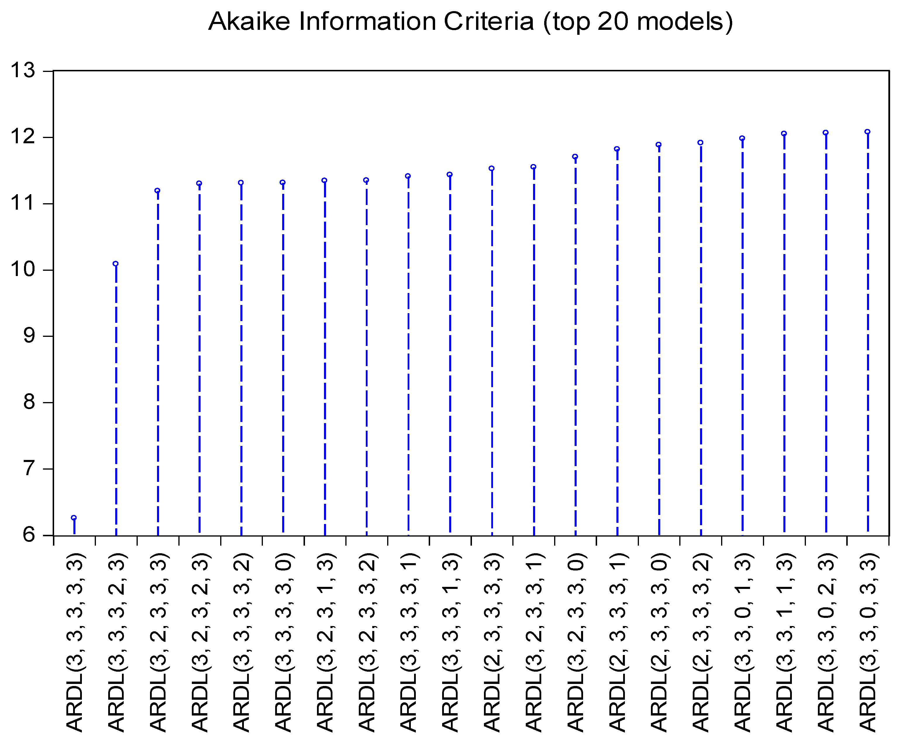
This condition was fulfilled, so the ARDL method to select the optimal equation model for the analysis was applied (Figure 5).

In total, 768 models were tested and the selection of the optimal model was made based on the graphical results using Akaike info criterion (AIC). It is essential to establish the optimal lag for each variable. The evaluation results show that the optimal analysis model is the one with three lags for each proposed variable.

After this step, a Bound test was applied to establish if there is a cointegration relationship between variables in the model. The results of these tests are presented in the

Table 4. ARDL cointegration analysis—Bound test.

	Estimated Models		LAG	F-Statistics
Romania	F(GHG/RET, RTT, RTPR, GGEXP)		3,3,3,3,3	168.17
	F(RET/RTT, RTPR, GGEXP, GHG)		3,3,3,3,3	1493.94
	F(RTT/RTPR, GGEXP, GHG, RET)		3,3,3,3,3	366.91
	F(RTPR/GGEXP, GHG, RET, RTT)		3,3,3,3,3	1126.80
	F(GGEXP, GHG, RET, RTT, RTPR)		3,3,3,3,3	730.58
	Critical Value Bounds
	Significance (%)	I0 Bound	I1 Bound
	10	2.45	3.52
	5	2.86	4.01
	2.5	3.25	4.49
	1	3.72	5.06

Source: Authors’ own analysis.

.

If the calculated F-statistics associated to the Bound test is higher than the critical values at all levels of significance, then there is a cointegration relationship among the variables. As it can be seen, all values of F-statistics are above the critical values, so it can be concluded that there are four cointegrating vectors in the equation and that there is a long-run cointegrating relationship between the variables.

After the existence of a cointegration relationship between greenhouse gas emissions, revenues from environmental taxes (on energy, transport and pollution/resources) and expenses for environment protection, the ordinary least squares (OLS) approach was applied to see to what extent the environmental taxes and government expenditures explain the greenhouse gas emissions. Analysing the results reported in

Table 5. ARDL cointegration estimation.

Dependent Variables	Romania
GHG	coefficient		t-stat	p
	short-run estimates
RET	−4.489	0.503	−8.920	0.071 *
RTT	−7.010	0.993	−7.055	0.089 *
RTPR	−18.867	2.452	−7.694	0.082 *
GGEXP	0.003	0.000	6.358	0.099 *
	long-run estimates
RET	3.047	0.574	5.305	0.118
RTT	21.129	4.026	5.247	0.119
RTPR	−10.500	1.255	−8.366	0.075 *
GGEXP	−0.007	0.001	−7.535	0.084 *
ECTt-1	1.2365	0.3501	3.5317	0.1757

* at 10% level. Source: Authors’ own analysis.

, several aspects regarding the connection between variables can be formulated.

On a short run, all variables included in the model are statistically significant at the level of 10% according to p-value. This means that on a short run, there is a cointegration relationship between the level of greenhouse gas emissions, environmental tax revenues and government spending on environmental protection. Thus, the Hypothesis no 1 is verified, according to which a growth in the revenues from taxes determines a decrease in greenhouse gas emissions in Romania.

On a short run, the total general government expenditure for environment protection does not have an effect on decreasing the greenhouse gas emissions, due to the fact that its efficiency in Romania is still very low. However, even if the financial funds for this type of expense are insignificant, they will have to increase in Romania, in order to attain the proposed sustainable development goals.

Regarding the relationship among long-term variables, it can be revealed that, in terms of green taxation, only the revenues from the taxes on pollution/resources have a statistically significant influence on greenhouse gas emissions. However, Hypothesis no 2 is validated, according to which government expenses on environmental protection determine a decrease in greenhouse gas emissions on a long-run, in Romania.

CUSUM and CUSUMsq tests were used to test the stability of the model. These tests are based on the cumulative sum of the recursive residuals. CUSUM test plots show the cumulative sum together with the 5% critical lines. The test identifies the parameter instability if the cumulative sum goes outside the area between the two critical lines. The graphical results for CUSUM and CUSUMsq tests show the stability of the parameters both on a long run and a short run, at a level of significance of 5% (Figure 6).

The existence of a cointegration relationship between the variables of the model implies the existence of a causality relationship at least in one direction. To determine the causality relationship between greenhouse gas emissions, revenue from taxes on energy, revenue from taxes on transport, revenue from taxes on pollution/resources and total general government expenditure for environment protection, the Granger test based on ARDL-ECM framework was used. This test shows whether there is a short-run, long-run or strong causality between the variables. To explain the long-run causal effects, the t-statistics of the ECT is analysed. If the value of t-statistics is negative, then there is a long-run relationship among variables.

According to the results from

Table 6. The ARDL-ECM Granger causality analysis in Romania.

	Dependent Variables
	D(GHG)	D(RET)	D(RTT)	D(RTPR)	D(GGEXP)
ECT(-1)	−0.375400	0.493629	0.026136	−0.061858	−160.0900
t-stat	[−3.15445]	[3.83430]	[0.91407]	[−5.61654]	[−1.48602]
D(GHG(-3))	−0.379603	0.578735	0.035850	−0.065192	105.0517
p-value	-	0.0142	0.4846	0.0015	0.5865
D(RET(-3))	−0.147158	−0.007187	0.004421	0.022166	−0.980768
p-value	0.3967	-	0.9154	0.1697	0.9950
D(RTT(-3))	−2.729777	0.513739	−0.152829	0.061367	−187.2354
p-value	0.0169	0.6710	-	0.5533	0.8531
D(RTPR(-3))	−2.274281	−0.289954	−0.595595	0.252645	−568.2124
p-value	0.0710	0.8294	0.0496	-	0.6142
D(GGEXP(-3))	−0.000357	0.000846	−6.40 × 10−5	5.36 × 10−5	0.399149
p-value	0.4717	0.1174	0.5904	0.2440	-

Is significant at the 0.01 level. Is significant at the 0.05 level. Source: Authors’ own analysis.

, there is a long-run existence of a cointegration relationship between pollution/ resources tax revenues and greenhouse gas emissions, as well as a cointegration relationship between the governmental expenses on environment protection and greenhouse gas emission (Hypothesis no 2).

For the long-run relationships between the variables, the t-statistic on the coefficient of the lagged ECT indicates that there is Granger-causality. The ECT relates to the fact that last period deviation from long-run equilibrium influences the short-run dynamics of the dependent variable. Thus, the coefficient of ECT is the speed of adjustment, because it measures the speed at which GHG returns to equilibrium after a change in the variables of the model. In the current case, the previous periods’ deviations from long-run equilibrium are corrected in the current period at an adjustment speed of 37.5%.

On a short run, several causal relationships between the variables included in the model are identified. Thus, there is a strong bidirectional causal relationship between pollution/resources tax revenues and greenhouse gas emissions. Another short-term causal relationship is identified from greenhouse gas emissions towards energy tax revenues, for the fact the energy consumed in Romania comes from traditional sources, with a major negative impact on the environment. In addition, the causality relation of the revenues from transport taxes on the greenhouse gas emissions is also significant. An increase in these revenues determines a decrease in the level of greenhouse gas emissions, being well known that the pollution from transport activities is major, because of the old transportation means and the use of fuels with a high negative impact on the environment, in Romania.

The previously obtained results were connected with the results obtained by applying Pairwise Granger causality test to detect the direction of causality on the long-run and short-run relationship between the variables in the model (Figure 7).

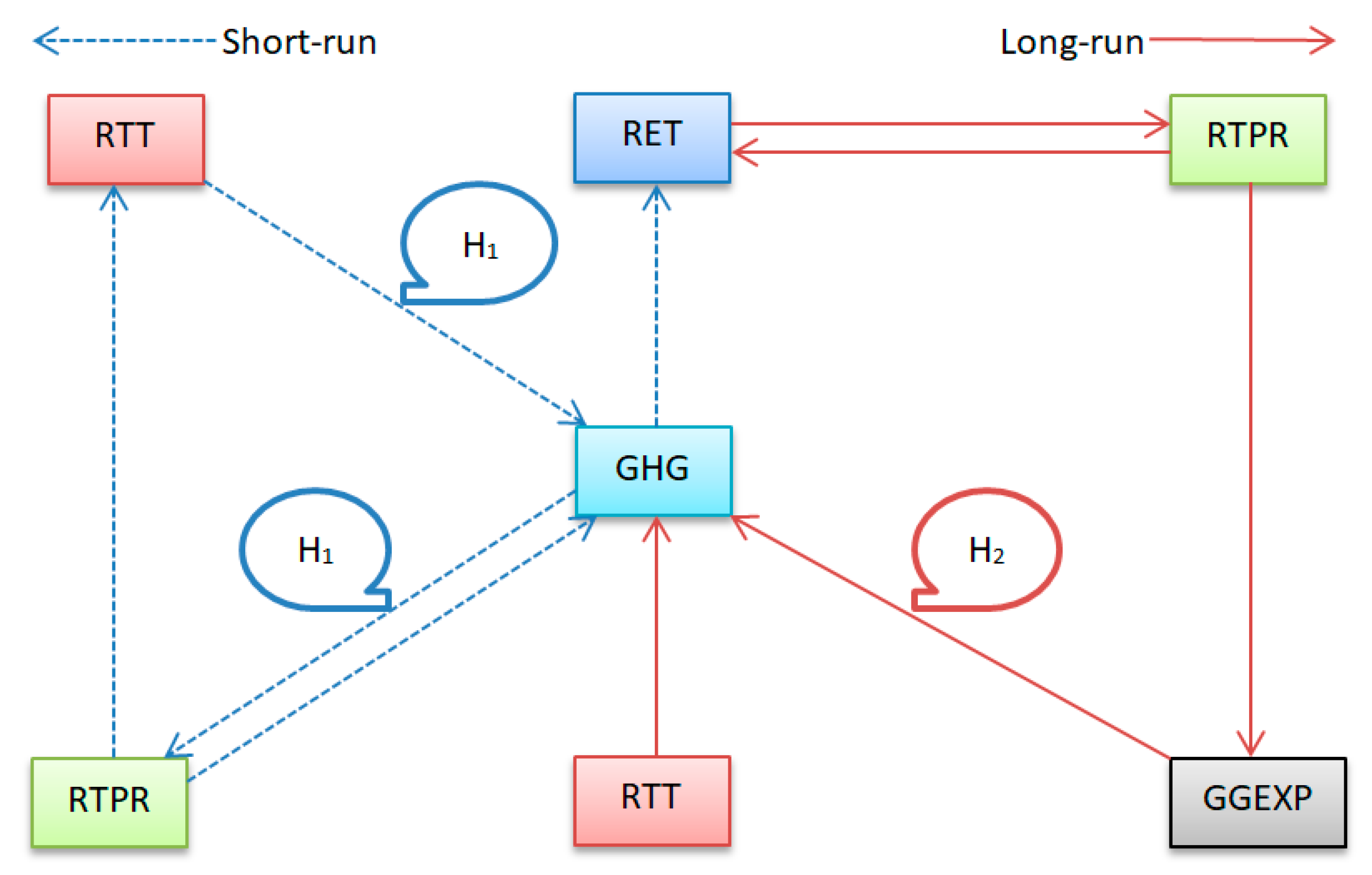
Thus, two bidirectional causality relationships have been identified, one on a short term between greenhouse gas emissions and revenues from taxes on pollution/resources and one on a long-term, between revenues from taxes on energy and revenues from taxes on pollution/ resources. In addition, on a short term, three other unidirectional causality relationships were identified: from revenues from taxes on pollution/resources towards the revenues from taxes on transport; from revenues from taxes on transport towards greenhouse gas emissions (which confirms the Hypothesis no 1) and from greenhouse gas emissions towards the revenues from taxes on energy.

In the long run, three unidirectional causal relationships have also been identified, namely: from revenues from taxes on pollution/ resources towards the total governmental expenses on environment protection; from government expenses on environment protection towards greenhouse gas emissions (Hypothesis no 2 is confirmed) and from revenues from taxes on transport towards greenhouse gas emissions.

5. Conclusions and Practical Implications

Countries’ pollution, climate change, weather disasters, global warming represent challenges that the states have been struggling with during decades, still less successfully, given the evolution of these issues lately. This paper analyses the causality between GHG emissions, the revenues from taxes on energy, transportation and pollution/resources and government expenditure on environment protection. This relationship is important because it offers a better understanding of the way GHG emissions can be reduced on both short and long run, using fiscal and budgetary policies.

Upheld on a time series of 23 years, from 1995 to 2018, the data being taken from the official website of the European Commission, Eurostat, and the theories regarding the role of environment taxes (the theory of the first dividend and the theory of the Kuznets curve), together with the implication of the national public authorities on the step towards a sustainable economic development, the findings provide valuable insight, leading to feasible solutions for reducing the pollution of the environment. The results are based on an equation that fragments the environment taxes on sources of origin and also includes the general government expenses for environment protection, a variable that has not previously been analysed in Romania.

The main results highlight two bidirectional causality relationships (one on a short term between greenhouse gas emissions and revenues from taxes on pollution/resources and one on a long-term, between revenues from taxes on energy and revenues from taxes on pollution/resources), three unidirectional causality relationships on a short run (from revenues from taxes on pollution/resources towards the revenues from taxes on transport; from revenues from taxes on transport towards greenhouse gas emissions and from greenhouse gas emissions towards the revenues from taxes on energy) and three unidirectional causal relationships on a long run (from revenues from taxes on pollution/resources towards the total governmental expenses on environment protection; from government expenses on environment protection towards the greenhouse gas emissions and from revenues from taxes on transport towards greenhouse gas emissions).

To sum up, the approached subject is of major importance and its aim is also to raise awareness of the concerned parties: researchers, practitioners, government representatives, policymakers, stakeholders, business environment and citizens. The efforts of experts from several fields, together with the collaboration among different industries are needed to overcome pollution and reach the lowest levels. In several other studies, it was shown that there is a strong significant correlation between the emissions of SO₂, NO_x and NMVOC and the industries of electric power, manufacturing and transport, in Romania [37]. Moreover, companies should implement sustainable indicators, with a positive impact on their financial performance [38]. The key implication of this study is that the environment taxes and the governmental expenses for environment protection on greenhouse gas emissions in Romania are underlined by the causality relationships among them. In this respect, governmental policies have to be supportive and innovative, in order to find the most adapted solutions to fight against these problems, since environmental tax regulations are widely used and adopted as the most important measures to reduce pollution as part of the governmental policies for environment protection.

The main limitations of the current research consist in the missing data in public official databases, together with the limited set of indicators that are published regularly. Consequently, the future research dimension can be oriented towards the connection between other environment protection taxes and the main governmental policies in this field. A particular attention shall be paid to make comparative analyses, using the same model in different states of the European Union for a larger period of time. However, the main pollutants: resources, transport and energy, in connection to the main governmental policies for environment protection will be analysed in the future research, using different research models, with new variables added. Other challenges that can be tackled in future research are related to the impact of environmental policies and fiscal measures meant to mitigate climate change on the performance of the companies. In order for the businesses to reduce their GHG emissions, they have to make important investments in nonpolluting technologies and equipment, all of these affecting their financial results, at least on a short term. Moreover, besides the environmental taxes, the focus will also be on other complementary research directions, such as sustainable development, from the perspective of “fulfilling the needs of the present generation, without compromising the future of generations to come” [39], while preserving the quality of life for the population [40].