

Abstract
The recent Environmental Research Letters article by Caesar, Rahmstorf and Feulner (hereafter CRF) is essentially a Comment on our Nature paper (Chen and Tung 2018 Nature 559 387–91), but without an accompanying rebuttal from us. In this unusual format for the exchange outside Nature, our rebuttal then becomes a Comment here at Environmental Research Letters. Our original proposal that the rate of global warming is enhanced by a weak Atlantic Meridional Overturning Circulation (AMOC) remains valid and is strengthened with this exchange. CRF used "established evidence" to argue against our finding, but such evidence is either misapplied (i.e. applying model results from preindustrial control runs with constant greenhouse gasses to the industrial era with increasing greenhouse gasses), or misinterpreted (i.e. climate model results for the industrial era specifically for the trends interpreted as for the AMOC cycles). While we used the observed energy budget to show that a strong (weak) AMOC transports more (less) heat to below 200 m, CRF replaces the actual budget with a simple energy-balance equation. They used an inappropriate equilibrium approximation to their simple equation to argue that global mean surface temperature (GMST) and AMOC should be in phase. We show here that the exact solution to that same equation actually supports our claim on the relationship between the rate of change of GMST and the AMOC state, which they misunderstood as we claiming a negative correlation between GMST and AMOC themselves. They claimed, incorrectly, that a positive correlation coefficient, no matter how small and even though none of them is statistically significant, is strong evidence that the two time series are in phase. The correlation coefficients that they found using observational data (0.01, 0.28 and 0.45), though positive, correspond to  out of phase, far from being in-phase. Visually they were made to look somewhat in-phase with decadal smoothing and short-period detrending. Both model and observational evidence supports the conclusion of our original paper that the period of AMOC minimum is a period of rapid rate of surface warming.
Export citation and abstract BibTeX RIS

Original content from this work may be used under the terms of the Creative Commons Attribution 4.0 license. Any further distribution of this work must maintain attribution to the author(s) and the title of the work, journal citation and DOI.
1. Introduction
In Chen and Tung (2018) (hereafter Chen and Tung) we suggested that the presence of the top-of-atmosphere (TOA) radiative imbalance due to increases in greenhouse gasses in the industrial era has changed the nature of heat transport of AMOC:
(A) We pointed out that existing evidence giving rise to the common perception that a weakened AMOC leads to cold Northern Hemisphere surface temperature was 'derived from model runs under preindustrial conditions' and 'paleoclimatology'.
(B) But it 'may not apply to modern era with our rapid emissions of greenhouse gases'. Instead 'the AMOC minimum was a period of rapid surface warming'. This comes about because the reduced heat sequestration into the deeper Atlantic during the AMOC minimum allows the greenhouse heating from above to warm the surface and the mixed layer of the oceans at a more rapid rate. Note that the quoted statement from Chen and Tung is about the rate of warming and the AMOC state. It is not a statement that GMST and AMOC were negatively correlated. We have never claimed that GMST and AMOC were anticorrelated. This is a serious misunderstanding on the part of CRF and might have contributed to their strategy of focusing on the sign of the correlation coefficient, no matter how small in magnitude.
Has CRF presented any evidence to contradict (B)? The answer is no, as we will elaborate.
CRF restricted their focus on the modern period of 1947–2012, but did not make any distinction between the preindustrial condition (A) and the very different condition of the modern era in the presence of rapidly increasing greenhouse gases (B). They incorrectly applied evidence, such as Knight et al (2005), based on long model runs under preindustrial condition with constant greenhouse gas concentrations, to the present climate to imply that our result is inconsistent with 'established understanding'. Our criticism of their work is not merely that they mixed up (A) and (B), but that their other lines of argument for the modern period are also incorrect.
Although CRF also quoted some studies that purportedly found a positive correlation between AMOC and GMST in the presence of rising greenhouse gases in the modern era, we will show in section 2 that the prior results have been misinterpreted. This misinterpretation is quite common in the community; so section 2 may be generally useful to a wider audience.
Our result in (B) for the present climate is new and need not conform to preindustrial evidence. We advanced the view that greenhouse warming, by creating a TOA radiative imbalance, has altered the dominant process of AMOC transport, from mainly a northward transport of surface heat from the tropics to high latitudes as in the preindustrial era, to a predominantly downward flux of heat in the Northern Atlantic in the modern era. New evidence for the current climate was established by Chen and Tung using the observed ocean energy budget. First, we showed that the sea-surface temperature (SST) co-varies with the ocean heat content (OHC) of the mixed layer on climate time scales down to a depth of 200 m globally. Therefore, if the OHC of the mixed layer increases (decreases), SST increases (decreases). CRF agrees with this point. The issue at hand then becomes that of the energy budget of the mixed layer: if there is more heat transported from the mixed layer to the deeper oceans below 200 m to be stored, OHC of the mixed layer (and SST) should decrease; otherwise it would increase. CRF disagrees with this conclusion and suggests that AMOC should transport heat upward, but no observational support was offered. This is refuted in sections 6 and 7 using observational evidence. While it may be true that, in a limited number of 'deep convection' sites in Labrador and Nordic Seas, very cold waters cooled by extreme cold air outbreaks may sink to below 3000 m and cool the abyssal ocean, Chen and Tung were referring to the Atlantic Ocean above 1500 m, and to a larger area means that could affect the global energy budget.
Our approach of using energy budgets establishes the causal relationship between ocean heat sequestration and GMST, and the effect of changing phase of AMOC on the partition of such heat storage. It is a physical, rather than a statistical evidence. It is much preferable to using the statistical method of correlation coefficients for a short data record adopted by CRF, which does not have causal information.
CRF used a simple energy balance model in place of our observed energy budget and seemed to have obtained a different result. We show in sections 3 and 4 that the exact solution to their simple model equation actually supports our conclusion. The problem lies in their inappropriate equilibrium approximation to their own equation.
CRF conflated our result on the part of the Atlantic above 1500 m with their idea on the relation of 'deep' ocean and 'deep convection'. We have clarified repeatedly in both our Science Article and Nature Letter what we meant by 'deeper Atlantic', and emphasized that we were studying the upper branch of AMOC using Argo data available above 1500 m. On the other hand, CRF used the terminology in oceanography where 'deep ocean' in the Atlantic refers to depths below 3000 m, the Abyssal Ocean, where we do not have much data, and did not draw any conclusion. This difference in terminology accounts for some of the confusion. Whether 'deep' convection actually cools the 'deep' ocean (below 3000 m), as asserted by CRF, is not the issue under consideration in Chen and Tung or here.
Another source of confusion is CRF's misuse of the term 'anticorrelation'. To help the readers better understand the issues under debate, it is useful to clarify before we begin what is meant by 'anticorrelation' and 'out of correlation'. In the simple case of two time series such as sin(t) and sin(t), which are in phase, we say they are perfectly correlated (with correlation coefficient 1). If the sign of one is opposite the other, we say they are anticorrelated (with correlation coefficient −1). If the time derivative of one of the time series is either positively or negatively highly correlated with the other time series, such as for the two time series: cos(t) and sin(t), we say that the two time series are out of correlation (with correlation coefficient equal to zero; or not statistically different from zero in real data). Mathematically, cos(t) and sin(t) are 90° out of phase, while sin(t) and −sin(t) are 180° out of phase. The latter is 'anticorrelated', but was not what was proposed by Chen and Tung.
2. Previous studies misinterpreted
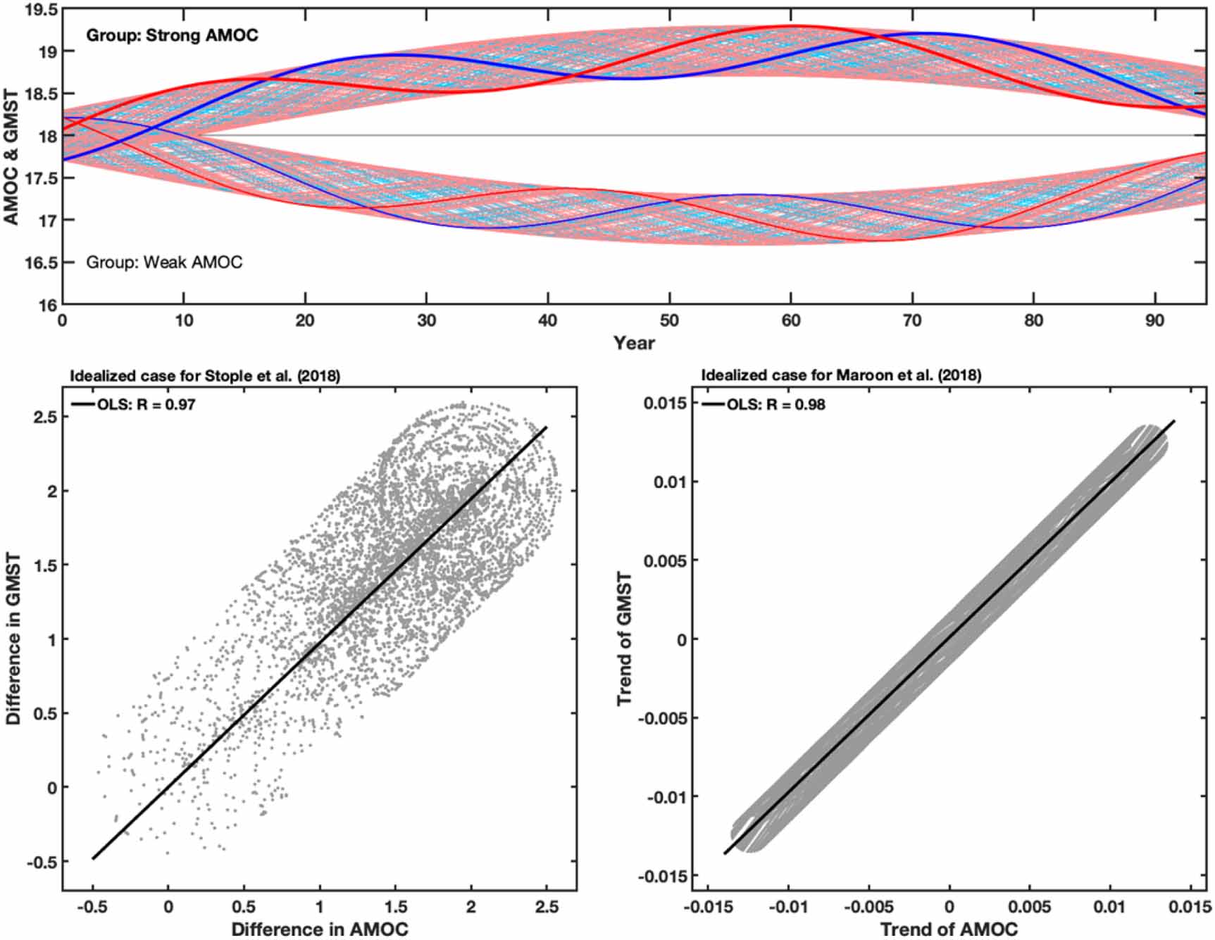
There have been several papers reporting climate model simulations that appear to show that a weaker AMOC leads to a cooler global surface temperature even in the presence of anthropogenic greenhouse gas forcing. Some of them have been quoted by CRF as supporting evidence. These reports need to be interpreted with care, because they may not be relevant to the issue at hand, which is the relationship between unforced multidecadal cycles of AMOC and GMST. For example, Maroon et al (2018)'s conclusion that 'there is a positive relationship between global surface warming and AMOC strength', quoted by CRF, was actually referring only to the trends and not to the relationship between GMST and the AMOC cycles. Their figure 4(b) only shows that the 75- year trends of AMOC and 75-year trends of GMST are positively correlated. Drijfhout (2015)'s figure 2(a) refers to the difference of two ensemble means; ensemble means eliminated the AMOC cycle and the related cycle in surface temperature. Hu et al (2011, 2013)'s results were also based on the differences of ensemble means. The result of Stolpe et al (2018) (their figure 5(b)), quoted by CRF, apparently showing a positive correlation of AMOC strength and GMST, was actually a correlation of the difference of AMOC strength and difference of GMST between two ensemble groups, one comprised of 'strong AMOC' as measured by its positive 100-year trend and another 'weak AMOC' group as measured by its negative 100-year trend. Since the overall ensemble mean was removed, there in principle should not be a trend or forced variability, but the grouping criterion created a positive (nonlinear) 'trend' in the 'strong AMOC' group, and a negative 'trend' in the 'weak AMOC' group. A similar situation applies to the case of Maroon et al (2018), except they used the difference between the 'strong AMOC' group and the overall ensemble mean.
To demonstrate how results similar to Stolpe et al (2018), Maroon et al (2018), Drijfhout (2015) and others can be misinterpreted, we repeat their procedures of analyses but with synthetic time series where the AMOC cycles and GMST are known to be 90° out of phase (i.e. one is a sine and the other is a cosine of the same phase) (figure 1(a)). Each pair of AMOC and GMST has a random phase, which generates the individual ensemble members. The upper group ('strong AMOC group') rides on a positive nonlinear trend and the lower group ('weak AMOC group') rides on an equal but opposite nonlinear trend, similar to Stolpe et al (2018)'s figure 4(b). The nonlinear trend here is from a part of a long (200 year) cycle of internal variability. For such long periods, the energy balance between ocean circulation and surface temperature could be taken as at equilibrium, and these nonlinear 'trends' taken as a slowly varying mean state. Differencing the two groups doubles the trend. The correlation between the difference of GMST and the difference of AMOC found by them is mostly the correlation between the long-term 'trends', obtained by the grouping. This high positive correlation, close to 1, is also found here (figure 1(b)), even though we know the correlation between cycles of AMOC and GMST should be zero by construction. Using this same synthetic example but applying to the case of Maroon et al (2018), no difference of the two groups is taken, and only the 'strong AMOC' group is considered. Plotting 75 year trends of GMST vs AMOC in figure 1(c) again shows a high positive correlation, again close to 1, even though we know the actual cycles should have zero correlation. These results show how such claimed positive correlation between AMOC and GMST can be misinterpreted.

Figure 1. Top panel: synthetic time series of AMOC (red) and GMST (blue). The heavy curves are for AMOC and GMST when the random phase is 0, and the light red and blue curves are ensemble members generated with random phase added. The blue and red members for each phase are exactly 90° out of phase (one is a sine and the other is a cosine). Lower left panel is obtained using the same procedure as Stolpe et al (2018). The difference of AMOC/GMST is obtained by the difference of a randomly selected pair of AMOC/GMST members, one from the 'strong AMOC' group (and its corresponding GMST) and one from the 'weak AMOC' group (and its corresponding GMST). The small time mean of the difference is removed before doing the correlation. Lower right panel is obtained using the same procedure as Maroon et al (2018), using only the 'strong AMOC' group. Different 75 year periods are defined by shifting the beginning of the period by one month. Then the linear trends of AMOC and GMST are calculated for each ensemble member. In both cases, the correlation coefficient between AMOC and GMST is almost 1, despite the fact that the synthetic AMOC and GMST cycles are 90° out of phase.
Download figure:
Standard image High-resolution image3. Observed and modeled relationship between AMOC and GMST
Observational data (figure 3 of Chen and Tung) is reproduced here as figure 2(a). The original data period was 1850–2017; only the section 1947–2012 is shown here. This is the period considered by CRF. During the period of weak AMOC, which transports less heat out of the mixed layer to the deeper ocean, the observed rate of GMST increase is more rapid. On the other hand, the rate of warming slowed when AMOC is strong. Figure 2 (b) is intended to show that the derivative of GMST is correlated with the AMOC index. But since the derivative of observational time series is highly fluctuating, what is shown in figure 2(b) is the integral: GMST vs the accumulation of AMOC. It shows convincingly that these two are negatively correlated. In other words, the rate of change of one time series is negatively correlated with the other series. The two time series themselves are therefore close to 90° out of phase. This is similar (but not exactly so) to the case of two time series, one a cosine and the second a sine: the derivative of the first is - sine, which is negatively correlated with the second time series, with a correlation coefficient of −1 (of course the observed time series are not so perfectly correlated.) A weak AMOC corresponds to a rapid rate of warming of GMST, which was the thesis of Chen and Tung.

Figure 2. Left column: observation. Right column: exact solution of equation (1). Upper row: GMST (in black) plotted with various normalized AMOC indices. Observed GMST is decadally smoothed using empirical mode decomposition (EMD) as described in Chen and Tung (2018). Lower row: same GMST (in black) plotted with the integral of various AMOC indices, normalized, showing the anti-correlation of the integral of AMOC with the multidecadal variability (MDV) of GMST. The observed MDV, T ', is GMST with the long-term (1850–2012) secular trend subtracted. The modeled T ' is GMST with the radiatively forced trend removed. The shade areas denote periods of warming slowdown and the unshaded area the period of accelerated warming, defined consistently in both observation and model solution by when T ' is declining and increasing, respectively. CRF did not use an objective criterion for shading.
Download figure:
Standard image High-resolution imageThe right two panels of figure 2 show the exact solution of CRF's equation (1) without the incorrect equilibrium approximation that they made. The exact solution shows that the AMOC minimum corresponds to a more rapid rate of increase in GMST (figure 2(c)), as in our original observation (here as figure 2(a)). The correlation of T ', which is GMST with the secular trend removed, and the accumulation of AMOC (or equivalently the correlation of  and AMOC), is −0.9, which is highly statistically significant because the model solution has many more cycles than shown. Our original observation result and simple model solution here are consistent with each other, in fact with very good agreement, in contrast to the claim by CRF that the two contradict each other. This refutes CRF's second argument based on the simple model. See section 4 for details of the exact solution.
There is a lag of  between GMST and AMOC as can be seen in figures 2(c) and (d). If this lag were
  , the correlation of
  and AMOC would have been −1, and that for T ' and AMOC would have been zero. In the present case the correlation coefficient for T ' and AMOC is nonzero, at −0.43. The behavior of the solution is closer to that for a lag of
  because
  is closer to
  . The simple-minded argument that if there is a nonzero correlation of T ' with AMOC then the two must be in-phase, is seen to be fallacious.
4. Exact solution of CRF's simple energy-balance model
CRF used a simple energy balance model, equation (1), in place of the actual energy budget:

Here, T is GMST, assumed to be the same as the mixed layer temperature, cm is the heat capacity of the ocean mixed layer, the atmospheric heat capacity being negligible in comparison, Qrad the radiative forcing and Qocean the heat transport across the bottom of the ocean mixed layer (fluxes are positive downward). Δ indicates differences to a previous equilibrium state (e.g. preindustrial). The term λ ΔT represents the equilibrium response of surface temperature to the forcing anomaly, which depends on the climate feedback parameter λ.
CRF proposed equation (2) as their balance, by dropping the left-hand side of equation (1):

The equilibrium assumption precludes any phase difference except 0 and  . That is, GMST and AMOC can only be perfectly in phase or oppositely signed.
However, the relevant case at hand is instead case (B), which is the one studied by Chen and Tung for the current climate when ΔQrad is an increasing function of time, and the climate state is not at equilibrium because there is a TOA radiative imbalance. So CRF's equation (2) and the implied balance of terms 'may not apply to modern era with our rapid emissions of greenhouse gases' (Chen and Tung 2018).
The full equation can be solved exactly keeping all terms, and the solution is as follows. For a linearly increasing radiative forcing and a sinusoidal AMOC variation:
 the analytic solution to equation (1) is:
where  is the initial condition. The primed quantities are dimensionless and defined by

The heat capacity of a global mixed layer of depth dm ∼ 200 m is
There are various definitions of the mixed layer depth. In this zero-dimensional model, equation (1), where the temperature of the mixed layer is assumed to be the same as GMST, the mixed layer depth should be defined as the maximum depth of the global upper ocean whose OHC covaries with global-mean SST. Chen and Tung found that this depth is 200 m, where the OHC covaries with SST with a correlation coefficient of 0.8.
In CRF's equation (1) the parameter depends on climate sensitivity, i.e. inversely proportional to equilibrium climate sensitivity (ECS). For a commonly accepted ECS value of 3 K (defined as the GMST response to a doubling of CO2), λ∼ (3.7/ECS) W m−2K−1 ∼ 1.2 W m−2 K−1. Therefore
  . The correlation coefficient is not sensitive to the value of
  .
.
This solution is plotted in figure 2(c) starting at  , when the influence of the initial condition is negligible. It bears no resemblance to CRF's equilibrium solution but agrees very well with our observed result in figures 2(a) and (b).
CRF's equation (2) is valid only at equilibrium: As stated by them, the symbols mean the difference between the new equilibrium and the previous equilibrium. But at such an equilibrium, the ocean heat flux out of the mixed layer should be zero. Equation (2) is then the well-known statement based on radiative balance models with a slab ocean (without ocean dynamics): In response to greenhouse gas heating increase, the Earth will increase its long-wave radiation to space by eventually attaining a higher equilibrium surface temperature. In the current climate, there is a TOA radiative imbalance, which is positive. This imbalance is accounted for by oceans transporting heat downward, and the situation is not at equilibrium.
The global energy balance of equation (1) lacks meridional energy transport. It does not contain the mechanism whereby northward transport of heat by AMOC keeps subpolar Atlantic warm, which is a dominant mechanism in the preindustrial era. Paradoxically it was also used by CRF to argue for the importance of meridional transport in the modern era. Chen and Tung suggested that in the modern era with net radiative driving, downward heat transport becomes the dominant mechanism. So equation (1) presumably could be applied to the current climate, but in this case it should not be at equilibrium. CRF's equilibrium approximation yields a correlation coefficient of −1 between T ' and AMOC unless heat is transported upward by a stronger AMOC. Whether heat is transported upward or downward by AMOC will be further discussed in sections 6 and 7.
5. Positive correlation coefficient does not mean in-phase relationship
It is difficult to infer phase relationship between two oscillations, say  , by examining only the sign of its correlation coefficient, except for the special cases when their phase difference
  is
is  . In other cases, which are the most often encountered ones, a positive correlation does not mean that the two timeseries are in phase, as can be shown. The correlation coefficient is:

which is positive for a range of phase differences:  . Similar argument applies for negative correlation. By definition, the two time series are in phase for
  . Then the correlation coefficient is 1. While a statistically significant correlation coefficient near 1 could mean that the two time series is close to being in phase, how does one interpret a correlation coefficient of 0.4?
A positive correlation coefficient does not necessarily imply that the two time series are in phase. Most of the correlation coefficients are below 0.5 in CRF's table 1 and close to zero in table 2, except those calculated for the unlikely large values of  . In reading CRF's tables, one should read only the first two columns of values for the correlation coefficients. CRF considered a range of
  . The high value corresponds to a low ECS of 1.2K, which was deemed by IPCC to be unlikely. In fact, any ECS below 2.2 K was recently found to be unlikely (Cox et al
2018). These unlikely values correspond to
. The high value corresponds to a low ECS of 1.2K, which was deemed by IPCC to be unlikely. In fact, any ECS below 2.2 K was recently found to be unlikely (Cox et al
2018). These unlikely values correspond to  values 1.7 and higher in CRF's tables. CRF themselves pointed out that for the relevant case of decadal to multidecadal time scales,
  should be 1.5 and 1.3, respectively. These were used in the first two columns of their tables, which show generally small values of correlation coefficient, and statistically insignificant even by their own account. Both positive and negative correlations were found. This is very weak evidence and does not support CRF's claim that GMST and AMOC are in phase or even positively correlated.
CRF's figure 1 was produced using  , which is unrealistic as discussed above. The correlation coefficient of their radiatively adjusted GMST and their own AMOC proxy using HadISST is actually 0.01 (and negative in their table 2) for
  , a more realistic value. When other AMOC proxies were used, the correlation coefficients were found to be 0.28 and 0.45. These correlation coefficients correspond to a phase difference between the two time series of
  These are closer to
  and clearly demonstrate the fallacy of CRF's argument based only on the sign of the correlation coefficient. They should have realized that the sign could be positive even if the phase difference is close to, but not exactly
CRF employed a number of procedures to inflate the calculated amplitude of the coefficient. These include decadal smoothing, within-a cycle, second linear detrending (see the legend of their figure 1), and using unrealistically large values of  (corresponding to very small ECS deemed unlikely by IPCC). Regardless of what is indicated in the labels on long-term detrending or radiative adjustment of the trends, we have verified that a second linear detrending was used for all correlation coefficients in tables 1 and 2.
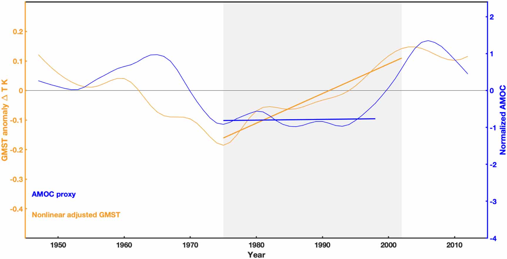
Detrending of surface temperature is sometimes used for the purpose of removing the anthropogenically forced radiative component. However, the trend that should be removed for this purpose should be the long-term trend in the industrial era. We used the observed long-term (1850–2012) secular trend to calculate the anthropogenically forced temperature response in Chen and Tung's figure 3, which is nonlinear but becomes more linear after 1910. Justifications were given in a long series of publications (Wu et al 2007, 2011, Tung and Zhou 2013, Zhou and Tung 2013, Chen and Tung 2017). Our T ', calculated as deviation from this long-term observed trend, is shown in figure 2(b), and is seen to be of opposite phase as the integral of AMOC. T ' has practically no linear trend over the recent 100 years, but has an apparent 'trend' over the shorter period shown due to the rising portion of the Atlantic multidecadal oscillation (AMO), an internal variability (Wu et al 2011, Chen and Tung 2017).

Figure 3. A cleaner version of CRF's figure 1. The shading is for the period when global warming accelerated, caused by the rising portion of the multidecal variability in GMST (MDV in Chen and Tung). Note that Chen and Tung's smoothed MDV was calculated for the long period of 1850–2017. Only the portion 1947–2012 is displayed here, away from the beginning and end of the data being smoothed. The color scheme is the same as that of CRF.
Download figure:
Standard image High-resolution imageAlthough decadal low-pass filtering of the time series can increase the magnitude of CRF's correlation coefficients, it also reduces their degrees of freedom. In a time series of 65 years, at most 6 degrees of freedom remain after decadal smoothing. After taking into account autocorrelation (Bretherton et al 1990), the degrees of freedom become 1.4–1.8 for the cases shown in CRF's table 1. The situation with their table 2 is even worse: for the shorter period considered there, AMOC is of one sign, at its minimum, hardly appropriate for establishing the correlation of cycles. Most of the values reported by CRF in both table are not statistically significant by their own account, and none is significant by our calculation; we were unable to reconcile the difference in the statistical calculations in our earlier exchange at Nature at manuscript stage. CRF's entries in the tables were unstable, and have changed in different versions of the manuscript.
Correlation coefficients were not used in Chen and Tung. Our argument was based on energy budget: When less heat is transported out of the mixed layer during the AMOC minimum, the OHC in the mixed layer is increased more and quantitatively accounts for the rate of increase of GMST in the modern era. But CRF's argument seems to entirely rest on the sign of the correlation coefficient obtained by them. They took the curious position that statistical significance does not matter: 'The fact that most of the correlation values are not significant at the 5% level (this was tested using amplitude-adjusted Fourier transform (AAFT) surrogates) is also irrelevant for deducing that an AMOC weakening does not enhance surface warming, as it is sufficient to show that the coefficients are not negative.' The coefficients are actually negative in their table 2. But that is not the point. That the correlation coefficient merely being positive or negative does not imply anything definite about the phase relationship, unless they are close to 1 or −1 and statistically significant.
Although none of these correlation coefficients is statistically significant (including ours if we were to calculate them using the observed time series in figures 2(a) and (b)), visually the locally detrended GMST processed by CRF gives the impression that it is in phase with the AMOC index, and this was the purpose of CRF showing their figure 1. Problems associated with short-term detrending over less than one cycle of an oscillation are well known. See for example Wu et al (2007, 2011). In the present case, decadal smoothing together the short-term detrending changes the zero crossings of the time series by a decade. The T ' from Chen and Tung was not subjected to these visual procedures, but it is hidden within the other curves. We replot it here in figure 3 without the clutter of other curves. During the flat minimum of AMOC, T ' increased almost linearly, necessarily from a negative anomaly to a positive anomaly, since the mean is removed. It is inappropriate for CRF to focus on the negative portion of the rising T ' from 1975 to 1995, and claim that it is positively correlated with the flat negative portion of the AMOC. Chen and Tung explained the physical process of why AMOC's minimum tends to be prolonged and flat, and why the rise of GMST during AMOC minimum is more rapid. As AMOC strengthened after the end of its minimum, it arrested GMST's growth, which then peaked and started to slow down. The data quality of the decades in the 1950s and 1960s is poor, and consequently the various proxies differ from each other in their phases. Nevertheless, it generally shows declining T ' when AMOC is positive, with the rate of decline largest when AMOC is at its maximum.
6. Weak AMOC increases ocean heat uptake?
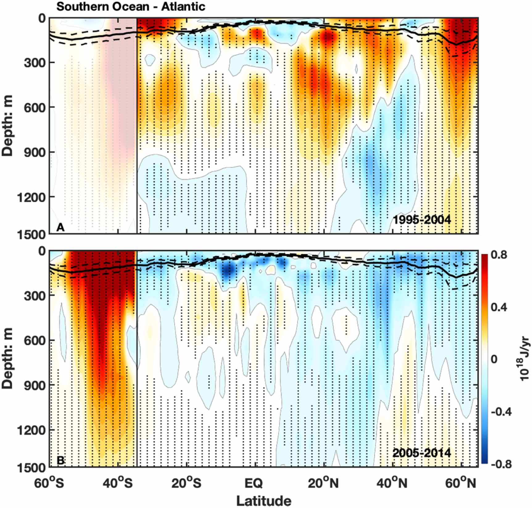
Subsurface meridional cross-section of the zonally averaged OHC linear trends in the Atlantic and the Southern Ocean are shown in figure 4, for the period when AMOC was increasing (4A) and when it was declining (4B). Note that linear trends show rate of change, and not the anomaly. This figure is similar to figure 4 in Chen and Tung, except zonal integral instead of zonal average is used here, and the mixed layer depth is superimposed. Adding up zonal integrals gives directly the contribution to the total OHC, already taking into account the different zonal widths of the Atlantic basin at each latitude.

Figure 4. Meridional cross section of OHC linear trends in North and South Atlantic, zonally integrated. (a) When AMOC is increasing, (b) when AMOC is declining. Regions where the signal is statistically significant above 95% confidence level are stippled. The Southern Ocean part in (a) is blanked out due to poor data before 2005. South of 35° S, the zonal integral is over a circumpolar channel without land. Winter mixed-layer depth calculated using Scripps subsurface Argo climatology (2000–2019) (in black curve), including its standard deviations (dashed curves), using the algorithm of Holte and Talley (2009) are superimposed upon the OHC cross section from Tung and Chen (2018).
Download figure:
Standard image High-resolution imageAfter a period of acceleration, AMOC started to decline since 2005, as observed by RAPID/MOCHA. Figure 4(b) shows that during this period AMOC's decline, subsurface Atlantic experienced a reduction of OHC throughout the Atlantic basin above 1500 m. The increase that CRF saw during the declining phase of AMOC comes instead from the Southern Ocean, defined as the circumpolar ocean south of 35° S. The increase in OHC in the Southern Ocean, however, started earlier, in the increasing as well as the declining phase of AMOC, as shown in figure 4 of our original paper using the thermosteric component of sea-surface height (SSH*) data available since 1993. Chen and Tung suggested that the warming of the subsurface Southern Ocean was caused by the Antarctic ozone hole's effect on the southward shift of the circumpolar westerly jet, which was a one-off event unrelated to AMOC variations.
Since observational data show that the warming of subsurface Southern Ocean started since at least 1993, it should not be attributed to the declining phase of AMOC. Data north of 35° S during the declining phase of AMOC, as presented in figure 4(b), directly contradicts CRF's claim that 'a weaker AMOC increases ocean heat uptake and therefore has a cooling effect on the global surface temperature'. The following statement by CRF is seen to be false: 'Additional support to this conclusion is provided by the fact that the recent decline of the AMOC coincided with an increase in the ocean heat uptake rate.' The OHC increase in the Southern Ocean was a separate phenomenon. CRF's figure 2 showing that the OHC increase, which they called 'ocean heat uptake rate', during the period 2005–2014 when AMOC decreased is misleading because it is not comparing the two time series from the Atlantic, and that the Southern Ocean's OHC was increasing even during the accelerating phase of AMOC, unrelated to its decline.
Furthermore, there is no mechanism that could have transmitted the signal of a declining AMOC from the Northern Atlantic to the Southern Ocean so quickly, in a matter of a few years. And Chen and Tung's figure 4, showing no movement of OHC between the action centers in the North Atlantic and the Southern Ocean, contradicts CRF's hypothesis of horizontal transport between the two oceans put forward in their figure 5.

Figure 5. Coincidence of the three AMOC phases with global warming slowdown and acceleration. (a) Global mean surface temperature. Black dots are annual mean values, and the red curve is smoothed version using EMD, same as in figure 2. (b) OHC north of 45° N in the Atlantic. Shown are averaged OHC in 5 m resolution in depth. (c) Salinity north of 45° N in the Atlantic. In (b) three AMOC proxies are superimposed: blue: Ishi + Scripps salinity proxy (Chen and Tung 2018); green: Subpolar SST index (Caesar et al 2018); black: subsurface fingerprint (Zhang 2008). Surface temperature data extends to 2017, but only up to 2012 is displayed. Modified and updated from the Extended Data Figure 3 of Chen and Tung.
Download figure:
Standard image High-resolution image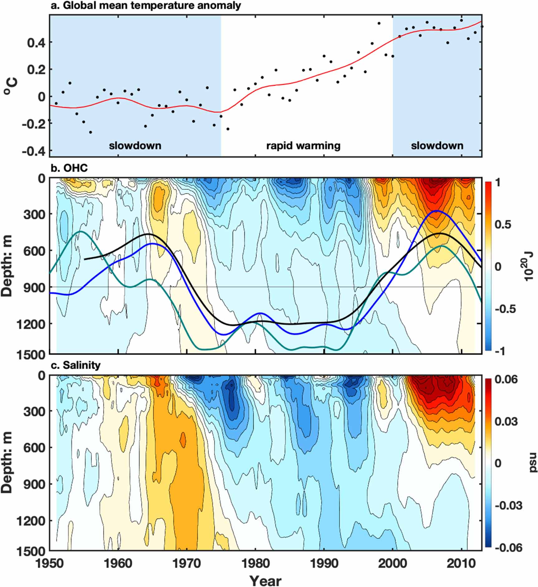
7. Heat transported downward or upward by AMOC?
Different terminology used by Chen and Tung (2018) and CRF may have caused this confusion. Chen and Tung defined 'deeper' Atlantic as the layer 200–1500 m, while CRF's 'deep ocean' refers to the abyssal ocean below 3000 m. Chen and Tung did not discuss whether the 'deep ocean' is cooled or warmed because the data we used did not extend below 1500 m.
Observational evidence shows that in terms of area-averaged and annually-averaged subsurface OHC, the subpolar Atlantic, including the open ocean, (and not just the limited regions of 'deep convection' sites referred to by CRF), is warmed by a stronger upper branch of AMOC in the 200–1500 m layer, as shown in figure 5. The figure shows that more heat and salinity are transported down below the mixed layer, to 900 m, when AMOC is stronger, and less when AMOC is weaker.
The downward transport of heat by a stronger AMOC is not limited to the subpolar Atlantic but is also significant in the subtropics and midlatitudes in the northward flowing upper branch of AMOC, as shown in figure 4. Warm saline water in the mixed layer in the subtropical Atlantic is transported northward as AMOC flows north and gradually sinks as it loses heat. At these latitudes the water is not cold enough to initiate 'deep convection', but cold enough for it to flow below the mixed layer to the 'deeper Atlantic' due to its salinity. These wider regions contribute more to the increase in OHC in the 200–1500 m layer than the subpolar region. (Subpolar Atlantic accounts for only 1/8 of the OHC increase below 200 m.)
The more saline water can sink even if the temperature is not as cold, thereby subducting some heat as it sinks. Such a thermohaline process may be thermally indirect. While a few episodes of extreme cold air outbreak during winter in limited areas of Labrador Sea and Nordic Seas may initiate 'deep convection' to below 3000 m, there are many more occurrences of less cold convection that do not reach that deep, but nevertheless transport heat to the 'deeper' Atlantic.
This definitive observational evidence is in contrast to CRF's unsupported claim of the opposite, which ignored salinity effects of the thermohaline convection. CRF argument was based only on the thermal effects, but it is known (Zika et al 2013) that 'heat can be pumped downward by the upper limb of the meridional overturning circulation through a combination of salinity gain in the subtropics and the mechanical forcing provided by Southern Hemisphere westerly winds'.
8. Discussion
In summary, we have refuted CRF's main points in two ways, (a) using observational data (see figures 2–5); (b) using the exact solution to CRF's simple energy balance equation but without their incorrect approximation (see sections 3 and 4). It should be noted that our original Letter did not use correlation coefficients to make our case, and we do not believe that the use of correlation coefficients by CRF can refute our result, since a statistical argument needs to rest on statistical significance, which they could not establish. Their argument is that a positive sign of the correlation coefficient between two time series implies in-phase relationship between the two series. This argument is shown to be false for correlation coefficient around 0.5 or less.
Our figure 4 here provides observational support that the ocean heat storage in the deeper Atlantic is increased when AMOC strengthened and decreased when AMOC weakened, the opposite of CRF's claim. Their claim was: 'Most model studies have shown that an AMOC decline, in response to increased CO2 concentrations, weakens the poleward ocean heat transport, increases the ocean heat uptake (Rugenstein et al 2013) and therefore diminishes global warming.' The only study cited actually does not support their claim. Rugenstein et al (2013)'s result is on the 100 year averaged difference of the responses of two closely related versions of the same model with minor differences in ocean mixing parameterization. These differences led to different magnitudes of northward heat transport but 'negligible' difference in ocean heat storage. The word 'ocean heat uptake' (OHU) used by Rugenstein et al (2013) has a different meaning than that used by CRF (such as in their figure 2). Rugenstein et al defined the OHU as 'the net downward surface heat flux (SFC), or OHU', while CRF used ocean heat uptake to denote increase in OHC storage below 200 m. In Rugenstein et al's experiment, as AMOC declines under 1% per year increase in CO2, AMOC weakens. There is no increase in the difference in ocean heat storage, but there is a decrease the northward heat transport, which then diminishes warming in the subpolar Atlantic. The less warm SST reduces the flux of heat from the ocean to the atmosphere at the subpolar surface, and therefore increases SFC (also called OHU in Rugenstein et al), which is measured as positive downward. On the other hand, throughout their article, CRF used ocean heat uptake to refer to the increase in OHC below 200 m. Furthermore, Rugenstein et al's 'warming' refers to the subpolar Atlantic ocean, not 'global warming' in CRF's quote of Rugenstein et al's conclusion. CRF is conflating Chen and Tung's result on the increase in ocean heat storage in the deeper Atlantic with Rugenstein et al's surface heat flux, thereby creating confusion with careless use of the phrase 'ocean heat uptake' throughout their article.
Our result is consistent with comprehensive coupled ocean-atmosphere models: if the greenhouse gases are held constant, surface temperature and AMOC strength should be in phase, as in Knight et al (2005), and should be close to 90° out of phase when greenhouse gases are rapidly increased, as in Kostov et al (2014) and Hu et al (2020). CRF's claim that 'over the last decades a weaker AMOC likely acted to delay global surface warming' runs counter to results from these two comprehensive climate model studies. Kostov et al (2014) studied the response of a suite of CMIP5 coupled climate models after CO2 is quadrupled and then held fixed. They found that the most important site of ocean heat uptake across models in the World Oceans is in the subpolar Atlantic: 'The depth and strength of AMOC are shown to be strongly correlated with the depth of heat storage across a suite of state-of-the-art general circulation models (GCMs). In those models with a deeper and stronger AMOC, a smaller portion of the heat remains in the ocean mixed layer, and consequently, the surface temperature response is delayed.' Hu et al (2020) compared two CMIP6 models with similar ECS and found: 'a weaker AMOC contributes in part to the higher transient climate response to a rising greenhouse gas forcing ... by permitting a faster warming of the upper ocean and a concomitant slower warming of the subsurface ocean. Likewise the stronger AMOC ... by permitting a slower warming of the upper ocean leads in part to a smaller transient climate response.'
Although most models predict weakening of AMOC under global warming, the observed variation of AMOC, which is likely natural and includes both acceleration and decline, is about ten times larger than model predicted decline under current conditions of greenhouse emissions (Chen and Tung 2018, Srokosz and Bryden 2015). In some models where the natural AMOC cycle is weaker than observed, forced increase in GMST occurs together with forced decline of AMOC, resulting in a negative correlation. This is not the relevant case discussed here, not by CRF (who proposed a positive correlation) nor us.
Acknowledgments
XC's research was supported National Science Foundation of China through Grants 41825012 and 41776032, and Basic Science foundation of Ocean University of China under Grant 202071001.
KKT's research was supported in part by the U. S. National Science Foundation through Grant NSF 1536175, and also by the Frederic and JuliWan Endowed Professorship.